Carbon and nitrogen dynamics in the coastal Sea of Japan inferred from 15 years of measurements of stable isotope ratios of Calanus sinicus

Both nitrogen and carbon dynamics have changed in the Sea of Japan. We hypothesized that the carbon and nitrogen stable isotope ratios (δ¹³C and δ¹⁵N) of the copepod Calanus sinicus could record changes in the coastal environment of the Sea of Japan. Consequently, these isotope ratios were monitored during the spring at four stations from 2006 to 2020 to identify the changes in carbon and nitrogen dynamics. The δ¹³C values ranged from −24.7 ‰ to −15.0 ‰ and decreased from the spring bloom (February–March) to the post-bloom (June–July) seasons. These variations were attributed to changes in the physiology of both C. sinicus and phytoplankton δ¹³C contents. The δ¹⁵N values range from 2.8 ‰ to 8.8 ‰, indicating that C. sinicus is a secondary producer; the tendency of the δ¹⁵N values to increase from the bloom to the post-bloom seasons was attributable to an increase in the δ¹⁵N of phytoplankton. A generalized linear model (GLM) approach indicated that >70 % of the variations in δ¹³C can be explained by sea surface temperature (SST), sea surface chlorophyll a concentration (SSC), carbon:nitrogen ratio of C. sinicus ($\mathrm{C}/\mathrm{N}$ ratio), and geographic differences. The residuals of δ¹³C in the GLM decreased yearly (−0.035 ‰ yr⁻¹). The GLM for δ¹⁵N of C. sinicus indicated that δ¹⁵N varies with the stage or sex in addition to SST, SSC, $\mathrm{C}/\mathrm{N}$ ratio, and geographic differences. The δ¹⁵N values of female C. sinicus and stage V copepodites were the lowest and highest, respectively. The residuals of δ¹⁵N in the GLM did not exhibit a significant interannual trend. These results suggest that the carbon isotope ratio in the secondary producer has linearly changed in the coastal Sea of Japan over the past 15 years. Moreover, the changes in carbon dynamics of this area have been recorded and observed to impact the marine ecosystem, while the nitrogen dynamics have not been recorded despite the increasing nitrogenous nutrient inputs in this sea.

1 Introduction

Coastal ocean ecosystems are ubiquitously important and have greatly changed as a result of human activities (Halpern et al., 2008; Doney, 2010). Stable isotope ratios of carbon and nitrogen have been employed to discern both the elemental cycles and environmental changes in marine ecosystems (Ohman et al., 2012; Lorrain et al., 2020; Ren et al., 2017), along with metrics of the trophic positions of organisms in an ecosystem (Aita et al., 2011). During the 21st century, the ¹³C:¹²C carbon isotopic ratio of tuna has rapidly been decreasing as a linear function with time, and the rate of decrease has been faster than expected owing to the Suess effect and the increase in anthropogenic carbon emissions (Gruber et al., 1999). Thus, it has been hypothesized that lower-trophic-level ecosystems have changed globally (Lorrain et al., 2020). In the marginal seas of East Asia, the ¹⁵N:¹⁴N nitrogen isotopic ratio of organic matter bound in coral skeletons has decreased with an increase in anthropogenic nitrogen deposition (Ren et al., 2017).

The Sea of Japan (Japan Sea) has been significantly impacted by human activities and global climate change (Chen et al., 2017). Monotonic changes have been detected in the chemical environment of coastal areas of the Sea of Japan, as well as in the global oceans (Ishizu et al., 2019; Ono, 2021; Kodama et al., 2016). In the surface waters of the Sea of Japan, pH and concentrations of phosphate and dissolved oxygen have been decreasing during the last few decades owing to global warming and the increase in atmospheric carbon dioxide (Ishizu et al., 2019; Ono, 2021; Kodama et al., 2016). The anthropogenic nitrogen inputs from the atmosphere have been increasing in the Sea of Japan (Kitayama et al., 2012), as well as in the global oceans (Duce et al., 2008). The Sea of Japan is regarded as an oceanic microcosm of the changing global ocean (Chen et al., 2017); thus, the impacts of changing inorganic chemical environments on biological production can be clearly detected compared to those in other oceans. Notably, the muscles of small pelagic fish in the Sea of Japan and the East China Sea from 1996 to 2019 showed that the annual mean ¹³C:¹²C and ¹⁵N:¹⁴N values monotonically decreased by 0.08 ‰ yr⁻¹ and 0.05 ‰ yr⁻¹, respectively (Ohshimo et al., 2021). This suggested a decrease in the stable isotope ratios of carbon and nitrogen in the food of small pelagic fish in the Sea of Japan. However, isotope values of both zooplankton and phytoplankton, which reflect the chemical environment in the Sea of Japan, have rarely been reported.

Calanus sinicus, the focus of this study, is a dominant copepod species in the coastal waters of the western North Pacific (Uye, 2000), including the Sea of Japan (Kodama et al., 2018a). Copepods of the genus Calanus are the major components of macrozooplankton in shelf and coastal ecosystems outside the tropics and are the major source of nutrition for pelagic fish (Uye, 2000). Maximum longevity of C. sinicus depends on the temperature but is usually less than 1 year (Uye, 1988); the development time from hatching to adulthood is ∼50 d at 10 ^∘C and 16 d at 20.2 ^∘C (Uye, 1988). The reproduction of C. sinicus occurs throughout the year but mainly at the end of spring or early summer (Huang et al., 1993; Zhang et al., 2005). The diapause phase is observed in the summer in the Yellow Sea (Pu et al., 2004b) but not in the Seto Island Sea of Japan (Huang et al., 1993). Calanus stores a large amount of lipid reserves during phytoplankton blooms (Gatten et al., 1980). The biology and ecology of C. sinicus in the Sea of Japan have been poorly studied, but the coastal areas of the Sea of Japan are spawning and nursery grounds for Japanese sardines (Sardinops melanosticta), Japanese anchovy (Engraulis japonicus), and Pacific bluefin tuna (Thunnus orientalis) (Nishida et al., 2020; Furuichi et al., 2020; Ohshimo et al., 2017); the larvae of these species prey on both the larval and adult stages of C. sinicus (Hirakawa et al., 1997; Hirakawa and Goto, 1996; Kodama et al., 2017a). Therefore, C. sinicus plays a vital role as a major component of the second trophic level in the Sea of Japan.

In this study, we hypothesize a decrease in carbon and nitrogen stable isotope ratios of C. sinicus in addition to that in small pelagic fish (Ohshimo et al., 2021), as the changing chemical environments in the Sea of Japan affected the marine ecosystem. Hence, we investigated the carbon and nitrogen stable isotope ratios of C. sinicus in the coastal area of Japan for 15 years in the 21st century and determined the controlling factors of stable isotope ratios using an empirical model approach. Subsequently, we calculated the long-term trends in the stable isotope ratios of C. sinicus to detect the impacts of the changing chemical environments in the Sea of Japan on the marine ecosystem.

2 Materials and methods

2.1 Onboard observations

Onboard observations were conducted from the pre- to post-bloom seasons from 2006–2020 during the R/V Mizuho-Maru, R/V Yoko-Maru (Japan Fisheries Research and Education Agency), and R/V Dai-Roku Kaiyo-Maru (Kaiyo Engineering Co., Ltd.) cruises in the territorial waters in the Sea of Japan, a marginal sea of the western North Pacific (Fig. 1). Four stations were chosen for the collection of stable isotope subsamples: Toyama Bay (TB), Iida Bay (IB), north of the Noto Peninsula (NN), and Wakasa Bay (WB). These four stations are among the 26 stations described in a previous study (Kodama et al., 2018a) that reported a clear west–east gradient of the zooplankton community structure with a temperature gradient in this area during May. Based on a previous study (Kodama et al., 2018a), the TB and IB stations were located in a cold-water area, and the NN and WB stations were located in a warm-water area. Additionally, the TB station was located near the mouths of two rivers (the Sho and Oyabe rivers; Fig. 1), and the WB station was in an area of restricted circulation. The cruises were conducted at four time intervals: (1) the end of February and/or the beginning of March (described as March), (2) the end of April, (3) the middle or end of May, and (4) the end of June or beginning of July (described as June) (Fig. 1c). The cruise in March corresponded to the early stage of the spring phytoplankton bloom; that in the April occurred during the late stage of the bloom, and those in May and June occurred during post-bloom conditions, according to Kodama et al. (2018b). Observations after 2015 were conducted only in April and May (Fig. 1c).

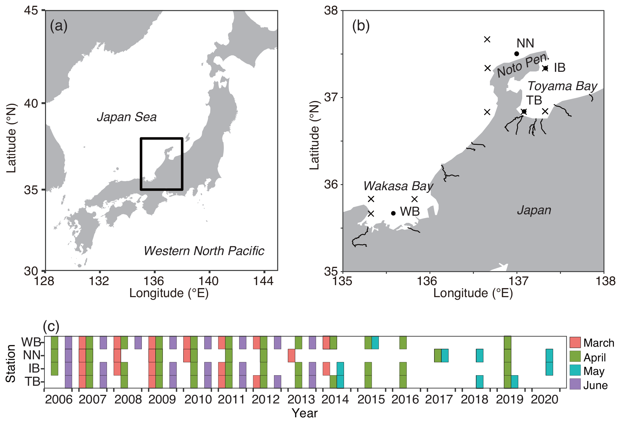
Figure 1 Sampling locations and dates. (a) Location of the study area in the Japan Sea. (b) Distribution of sampling stations of Calanus sinicus (closed circles) and particulate organic matter (POM) for stable isotope analysis along the Japanese coast of the Japan Sea. (c) Months and years of samplings of C. sinicus at the four stations. The lines in (b) denote the downstream reaches of class A rivers. The maps were made with Natural Earth and the Geospatial Information Authority of Japan.

Copepods for stable isotope analyses were collected by towing a bongo net (500 µm mesh and 70 cm mouth diameter) obliquely at 0.5 s⁻¹ from a depth of 75 m, or 10 m above the bottom, to the surface at each station. Collected samples were frozen and preserved at $\le -$20 ^∘C until sorting was conducted at an onshore laboratory. Some samples were stored for more than 10 years. Vertical profiles of temperature, salinity, and chlorophyll a concentration were measured using a conductivity–temperature–depth (CTD) sensor (Sea-Bird, SBE 9 plus, or SBE 19 plus) with an in vivo chlorophyll fluorescence sensor from a depth of 200 m to the surface. The temperature and salinity of the sensors were annually calibrated by the manufacturer. Surface seawater was sampled with a bucket to measure the sea surface temperature (SST), sea surface salinity (SSS), and sea surface chlorophyll a concentration (SSC). SST and SSS were measured with a calibrated mercury thermometer and salinometer (Autosal, Guildline Instruments), respectively. To measure the chlorophyll a concentrations, particles in 300 mL of water were collected on a glass fiber filter (GF/F, Whatman), and the pigments were extracted with N,N-dimethylformamide. Chlorophyll a concentrations were estimated based on the fluorescence of the extract, which was measured using a fluorometer (10-AU, Turner Designs) (Holm-Hansen et al., 1965). The chlorophyll fluorescence sensor was calibrated using discrete samples collected during each cruise. The nutrient concentrations at the surface were measured in cruises conducted after 2015. The procedures used for the nutrient analyses have been described by Kodama et al. (2015).

We collected and measured the stable isotope ratios of particulate organic matter (>0.7 µm, POM) in April 2017 (at 0 m depth, n=6) and May 2019 (at 10 and 30 m depths, n=6) near the C. sinicus sampling sites (Fig. 1b). Particles in 1.5–4.6 L seawater were collected on the pre-combusted (460 ^∘C, 6 h) glass fiber filter (GF/F, Whatman), which were frozen and stored until the analyses in the onshore laboratory.

All data and program codes are obtained from the Digital Commons Data (Nakamura et al., 2021).

2.2 Stable isotope analyses

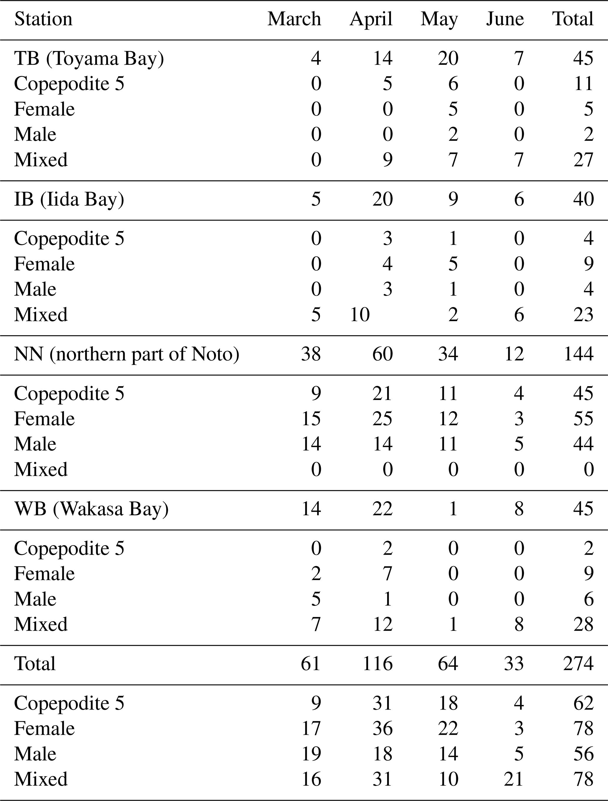
A total of 94 frozen Bongo net samples were thawed at room temperature. From each thawed sample, Calanus sinicus (Copepoda; Calanoida) adults or stage V copepodites were sorted as quickly as possible under a dissecting microscope to avoid their alteration or contamination. Calanus sinicus samples were soaked in a 3 % NaCl aqueous solution to clean their bodies. The 28 samples were divided into subsamples of stage V copepodite (C5), adult female (F), and adult male (M), and the remaining 66 samples were not divided. The physiological processes of C. sinicus differ according to their stage and sex (Zhou et al., 2016; Pu et al., 2004a, b). At least five individuals were necessary for measuring the stable isotope ratio in each subsample. When C. sinicus was present in one sample, several subsamples were prepared to evaluate the variability of the analysis. Therefore, a total of 267 subsamples were prepared to measure the stable isotope ratios. Each subsample was wrapped in a tin disk after drying at 60 ^∘C in a drying oven for 36–48 h. Table 1 presents the details regarding the number of subsamples. The stable isotope ratios of each subsample were measured.

Table 1 Numbers of subsamples of Calanus sinicus for stable isotope analysis.

The carbon and nitrogen stable isotope ratios of the subsamples were measured using a stable isotope ratio mass spectrometer (IsoPrime100; Elementar) coupled with an elemental analyzer (vario MICRO cube, Elementar). The stable isotope ratios of carbon and nitrogen were calculated in per mill (‰) deviations from the corresponding standards using the following equation:

$$\begin{array}{}\text{(1)}& {{\mathit{\delta }}^{\mathrm{13}}\mathrm{C}}_{\mathrm{bulk}}\text{or}{{\mathit{\delta }}^{\mathrm{15}}\mathrm{N}}_{\mathrm{bulk}}=\left[\right(R_{\mathrm{sample}}/R_{\mathrm{standard}})-\mathrm{1}]\times \mathrm{1000},\end{array}$$

where R is the ${}^{\mathrm{13}}\mathrm{C}{/}^{\mathrm{12}}\mathrm{C}$ or ${}^{\mathrm{15}}\mathrm{N}{/}^{\mathrm{14}}\mathrm{N}$ ratio, respectively. The standards for carbon and nitrogen were L-alanine, and the references were Pee Dee Belemnite and atmospheric N₂, respectively. The precision of the analysis was within 0.2 ‰ for both δ¹³C and δ¹⁵N. Based on the precision of the analyses of L-alanine, the δ¹³C and δ¹⁵N values for each subsample were rounded off to one decimal place. The amounts of carbon and nitrogen in each subsample were also recorded, and the carbon:nitrogen ratio ($\mathrm{C}/\mathrm{N}$ ratio) of C. sinicus was calculated. However, we did not conduct any lipid extraction processes. Lipids affect δ¹³C; however, lipid corrections are possible using modeling approaches (Logan et al., 2008). Thus, we calculated the lipid-free δ¹³C (δ¹³C_ex) based on the δ¹³C_bulk, $\mathrm{C}/\mathrm{N}$ ratio, and the equation reported by Smyntek et al. (2007).

Before measuring the isotope ratios of POM, the filters were exposed to HCl fumes for more than 2 h to remove carbonate salts. The decarboxylated filters were dried in an oven (60 ^∘C, overnight), and the entire filter was wrapped in a tin cup to measure the carbon and nitrogen stable isotope ratios, as well as the C. sinicus.

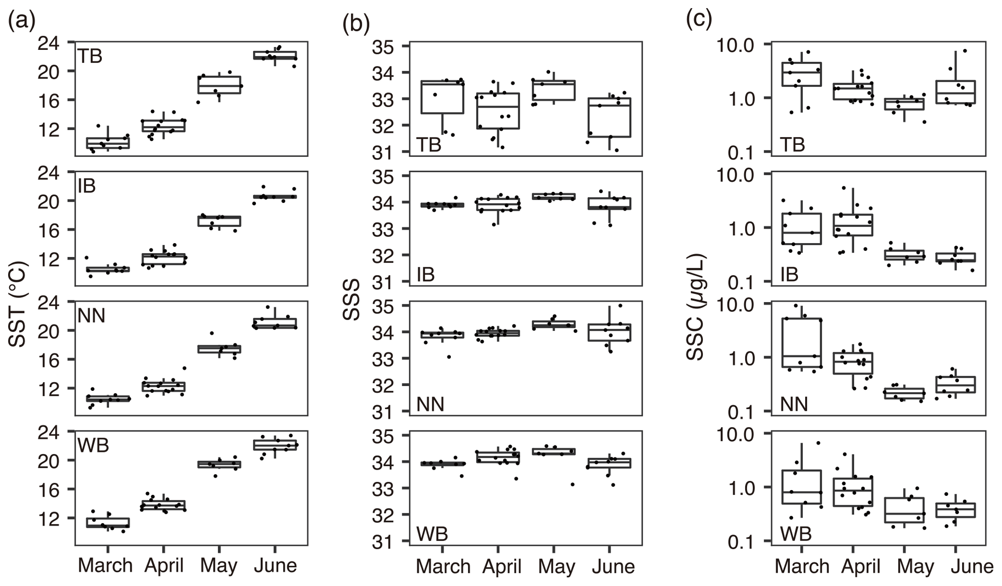
Figure 2 Variations of environmental parameters among months and stations. (a) Sea surface temperature (SST), (b) sea surface salinity (SSS), and (c) sea surface chlorophyll a concentration (SSC). Values at TB, IB, NN, and WB are shown. Box plots show the medians (horizontal lines within boxes), upper and lower quartiles (boxes), and quartile deviations (bars). Small points are raw data points. In (a), the lowest outlier at TB in March (SSS = 28) is not shown.

2.3 Statistical analyses

The relationships between δ¹³C_bulk and δ¹⁵N_bulk of C. sinicus and environmental parameters (SST, SSC, and SSS) were analyzed using general linear models (GLMs) with the linear link function using the R software (R Core Team, 2020). The structures of GLMs were based on the concepts articulated by Kodama et al. (2021). The δ¹³C and δ¹⁵N errors were assumed to be normal distributions, and explanatory variables were expressed as linear functions in the GLMs, with the exception of SSC, which was log-transformed. Two types of GLMs were applied as follows:

$$\begin{array}{}\text{(2)}& \begin{array}{rl}{{\mathit{\delta }}^{\mathrm{13}}\mathrm{C}}_{\mathrm{bulk}}\text{or}{{\mathit{\delta }}^{\mathrm{15}}\mathrm{N}}_{\mathrm{bulk}}& \sim \text{poly}(\text{SST},\mathrm{2})+\text{poly}(\text{log}\text{SSC},\mathrm{2})\\ & +\text{poly}(\text{SSS},\mathrm{2})+\text{poly}(\mathrm{C}/\mathrm{N},\mathrm{2})\\ & +f\left(\text{stn}\right)+f\left(\text{stage}\right),\end{array}\end{array}$$

where stn and stage represent the target δ¹³C_bulk or δ¹⁵N_bulk, station (WB, NN, IB, and TB), and copepod stages (C5, F, M, and mixed), respectively. The arguments of the f functions are categorical variables used to simulate nonlinear relationships. The second argument of the polyfunctions (i.e., 2) indicates that the first one was incorporated into a quadratic expression in the model; namely, dome-shaped responses were included in the models. We added the “mixed” stage category for the subsamples undivided into stage or sex categories. We applied this GLM approach to δ¹³C_ex; however, the results, except for the $\mathrm{C}/\mathrm{N}$ ratio, were very similar to δ¹³C_bulk, and thus the results of δ¹³C_ex are not shown. The significance of the parameters was checked by the analysis of variance (ANOVA). The explanatory variables in the final version of Eq. (2) were determined based on the values of generalized variance inflation factors (GVIFs) and Akaike information criteria (AICs). We required the GVIFs of the explanatory variables to be less than 10, and the model with the smallest AIC was accepted as the final model. For example, we did not apply f (month) and f (year) to the explanatory variables in Eq. (2) because they are collinear with other environmental parameters. The “ggpredict” function in the “ggeffects” package (Lüdecke, 2018) was used to visualize the effect of the explanatory variables on the δ¹³C_bulk or δ¹⁵N_bulk values. When categorical variables (i.e., stage and station) remained in the models with the least AIC, their values were fixed to calculate the predicted values.

We evaluated the monthly and interannual variations of the stable isotope ratios using the residuals (observation–prediction) of Eq. (2) (described as residual δ¹³C and δ¹⁵N). The trends of the residual δ¹³C and δ¹⁵N were expected to indicate the trend of δ¹³C_bulk and δ¹⁵N_bulk, excluding the interannual trends of environmental parameters and geographical effects.

3 Results

3.1 Environmental variables

The SST increased from March to June at every station (Fig. 2a). The SST at WB, the westernmost station, showed the highest SST among the four stations during every cruise. The SST ranges were 8.8–23.1, 9.5–21.9, 9.3–23.2, and 10.1–23.4 ^∘C at stations TB, IB, NN, and WB, respectively. The SSS was low at station TB (Fig. 2b). The ranges of SSS were 28.6–34.5, 33.1–34.3, 33.1–34.6, and 33.1–34.6 at stations TB, IB, NN, and WB, respectively. The SSS was the highest in May at the other three stations. Variations of SSC concentration at TB differed from those at the other stations. The SSC was higher at TB than at the other stations in every month. Additionally, the SSC at TB was higher in June than in May (Fig. 2c). The SSC values ranged from 0.02–7.45, 0.08–5.46, 0.05–9.07, and 0.08–6.60 µg L⁻¹ at stations TB, IB, NN, and WB, respectively.

The mean ± standard deviation of the $\mathrm{C}/\mathrm{N}$ ratio in C. sinicus was 5.5±2.6 g g⁻¹. The $\mathrm{C}/\mathrm{N}$ ratio in C. sinicus ranged from 3.4 to 19.2 g g⁻¹. The $\mathrm{C}/\mathrm{N}$ ratio was significantly different among the stages (ANOVA, p<0.001, degree of freedom = 3, F = 30.1); the $\mathrm{C}/\mathrm{N}$ ratio was highest in C5 (mean ± sd: 7.9 ± 4.0 g g⁻¹, n=61) and lowest in F (4.6±0.8 g g⁻¹, n=78). The monthly variations were also significant (ANOVA, p<0.001, degree of freedom = 3, F = 15.09); the $\mathrm{C}/\mathrm{N}$ ratios in all stages were the highest in April (Fig. 3a).

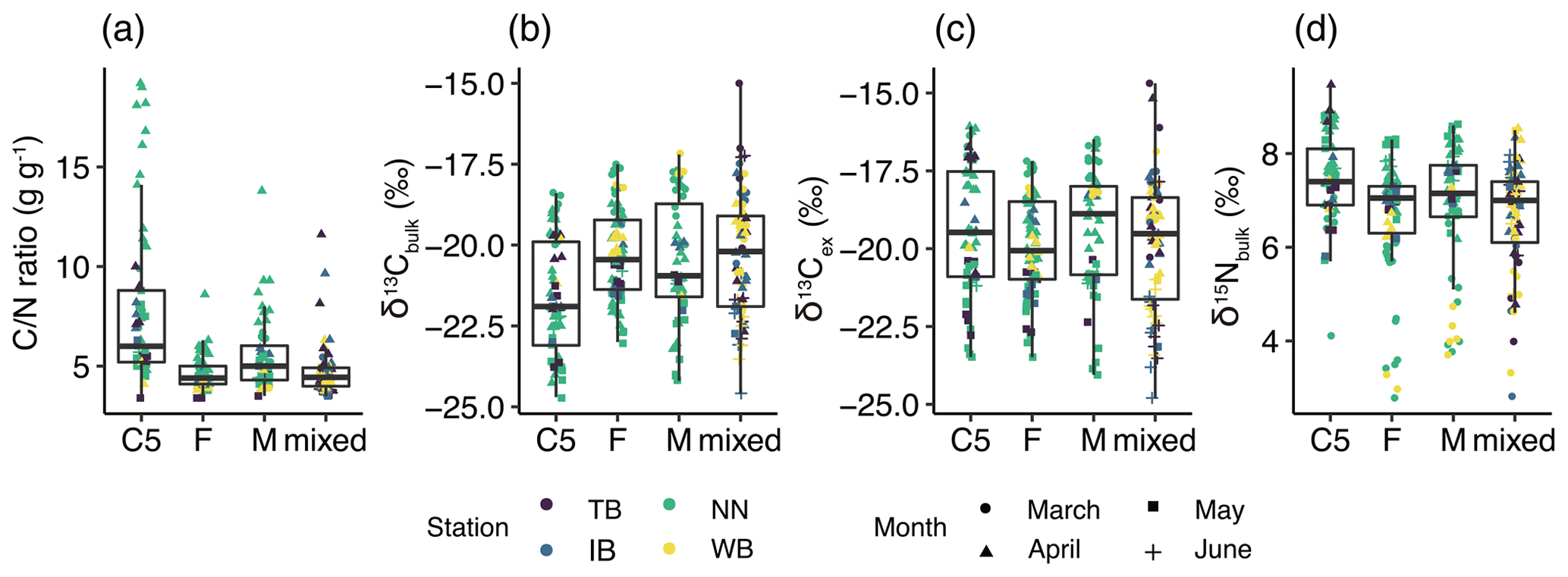
Figure 3 Variations of (a) $\mathrm{C}/\mathrm{N}$ ratio, (b) δ¹³C_bulk, (c) δ¹³C_ex, and (b) δ¹⁵N_bulk values in C. sinicus among growth stages and sex. The growth stages and sex of C. sinicus were divided into copepodite V (C5), adult female (F), adult male (M), and mixed (undivided). Box plots show the medians (horizontal lines within boxes), upper and lower quartiles (boxes), and quartile deviations (bars). Small points are raw data points, and the colors and shapes of points indicate stations and sampling months, respectively.

3.2 Stable isotope ratios and their relationship between environmental parameters

The δ¹³C of POM ranged from −27.3 ‰ to −22.5 ‰ (mean ± standard deviation: $-\mathrm{24.8}\mathrm{‰}\pm \mathrm{1.6}$ ‰) and from −24.9 ‰ to −23.0 ‰ (−23.7 ‰ ± 0.7 ‰) in April 2017 and May 2019, respectively. The δ¹⁵N of POM ranged 3.1 ‰ to 5.1 ‰ (4.1 ‰ ± 0.7 ‰) and 2.5 ‰ to 4.3 ‰ (3.5 ‰ ± 0.7 ‰) in April of 2017 and May of 2019, respectively.

The means ± standard deviations of all of the C. sinicus δ¹³C_bulk, δ¹³C_ex, and δ¹⁵N_bulk values were −20.6 ‰ ± 1.8 ‰ (−24.7 ‰ to −15.0 ‰), −19.6 ‰ ± 1.9 ‰ (−24.8 ‰ to −14.7 ‰), and 6.9 ‰±1.2 ‰ (2.8 ‰ to 8.8 ‰), respectively. The highest δ¹³C_bulk values were observed in March at all four stations (TB: −17.5 ‰ ± 2.1 ‰; IB: −18.7 ‰ ± 1.1 ‰; NN: −18.7 ‰ ± 0.9 ‰; and WB: −18.5 ‰ ± 1.1 ‰; Fig. S1 in the Supplement), and the lowest monthly mean δ¹⁵N_bulk was observed in March at all four stations (TB: 5.1 ‰ ± 0.8 ‰; IB: 5.1 ‰ ± 1.4 ‰; NN: 5.6 ‰ ± 1.3 ‰; and WB: 4.5 ‰ ± 1.0 ‰; Fig. S1). Comparing the δ¹³C_bulk values among the C. sinicus stages, those of C5 were significantly lower than those of F and M (Fig. 3b, Tukey's honestly significant difference – HSD – test, p<0.001), whereas no significant differences were observed in the δ¹³C_ex values between the stages (Fig. 3c, ANOVA, p=0.186). Comparing the δ¹⁵N_bulk values among the C. sinicus stages, those of C5 were significantly higher than those of F and M (Fig. 3d, Tukey's HSD test, p<0.017), and those of F, M, and mixed stages were at the same level (Tukey's HSD test, p>0.8). The δ¹³C_bulk, δ¹³C_ex, and δ¹⁵N_bulk values of C. sinicus in April 2017 were −21.6 ‰ ±  0.6 ‰, −18.2 ‰ ± 1.3 ‰, and 8.1 ‰ ± 0.6 ‰, respectively; those in May 2019 were $-\mathrm{23.7}\mathrm{‰}\pm \mathrm{0.1}$ ‰, $-\mathrm{22.2}\mathrm{‰}\pm \mathrm{0.1}$ ‰, and 6.7 ‰±0.4 ‰, respectively.

In the model with the least AIC, we used Eq. (2) to remove SSS from the full model for both δ¹³C_bulk and δ¹⁵N_bulk. Additionally, this stage was not selected in the least-AIC model of δ¹³C_bulk. Thus, the following equations represent the least-AIC models.

$$\begin{array}{}\text{(3)}& {\displaystyle }\begin{array}{rl}{{\mathit{\delta }}^{\mathrm{13}}\mathrm{C}}_{\mathrm{bulk}}& \sim -\mathrm{20.47}(\pm \mathrm{1.49})\times \mathrm{SST}+\mathrm{7.54}(\pm \mathrm{1.04})\\ & \times {\mathrm{SST}}^{\mathrm{2}}+\mathrm{2.82}(\pm \mathrm{1.54})\times \text{log}\mathrm{SSC}+\mathrm{0.70}(\pm \mathrm{1.16})\\ & \times (\text{log}\mathrm{SSC}{)}^{\mathrm{2}}-\mathrm{12.24}(\pm \mathrm{1.11})\times \mathrm{C}/\mathrm{N}\\ & +\mathrm{8.13}(\pm \mathrm{1.04})\times {\mathrm{C}/\mathrm{N}}^{\mathrm{2}}+f\left(\mathrm{stn}\right)\end{array}\text{(4)}& {\displaystyle }\begin{array}{rl}{{\mathit{\delta }}^{\mathrm{15}}\mathrm{N}}_{\mathrm{bulk}}& \sim \mathrm{9.11}(\pm \mathrm{1.48})\times \mathrm{SST}-\mathrm{7.46}(\pm \mathrm{1.03})\\ & \times {\mathrm{SST}}^{\mathrm{2}}+\mathrm{0.26}(\pm \mathrm{1.43})\times \text{log}\mathrm{SSC}\\ & -\mathrm{2.39}(\pm \mathrm{1.12})\times (\text{log}\mathrm{SSC}{)}^{\mathrm{2}}+\mathrm{3.97}(\pm \mathrm{1.27})\\ & \times \mathrm{C}/\mathrm{N}-\mathrm{0.46}(\pm \mathrm{1.05})\times {\mathrm{C}/\mathrm{N}}^{\mathrm{2}}+f\left(\mathrm{stn}\right)\\ & +f\left(\mathrm{stage}\right)\end{array}\end{array}$$

The coefficient of determination (r²) values of the least-AIC δ¹³C and δ¹⁵N models were 0.712 and 0.448, respectively. The effects of all variables were significant, except for the logSSC stage in δ¹⁵N_bulk (ANOVA). The dispersion values of both models were <1.

The least-AIC models produced convex graphs of δ¹³C as a function of SST or the $\mathrm{C}/\mathrm{N}$ ratio (Fig. 4a, c). The minima of δ¹³C_bulk values occurred at an SST and a $\mathrm{C}/\mathrm{N}$ ratio of approximately 20 ^∘C and 14, respectively (Fig. 4a, c). Inter-station comparisons indicated that the δ¹³C_bulk values were 0.6 ‰–1.1 ‰ higher in WB and TB compared to those in IB and NN (Fig. 4d).

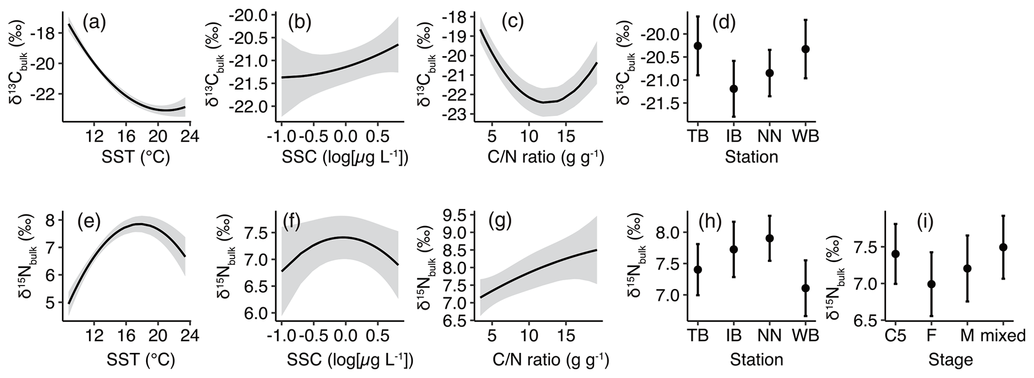
Figure 4 Responses of least-Akaike information criterion (AIC) generalized linear models (GLMs) based on least-squares mean (predicted) values. (a) δ¹³C_bulk versus sea surface temperature (SST), (b) δ¹³C_bulk versus sea surface chlorophyll a concentration (SSC), (c) δ¹³C_bulk versus carbon:nitrogen ($\mathrm{C}/\mathrm{N}$) ratio, (d) δ¹³C_bulk versus stations, (e) δ¹⁵N_bulk versus SST, (f) δ¹⁵N_bulk versus SSC, (g) δ¹⁵N_bulk versus $\mathrm{C}/\mathrm{N}$ ratio, (h) δ¹⁵N_bulk versus station, and (i) δ¹⁵N_bulk versus stages. Black lines with gray shading (a–c, e–g) or closed circles with vertical bars (d, h and i) denote the predicted values with 95 % confidence limits based on the GLMs.

The responses of δ¹⁵N_bulk to SST mirror those of δ¹³C_bulk to SST (Fig. 4e). The least-AIC model produced a concave graph of δ¹⁵N_bulk as a function of logSSC (Fig. 4f). The δ¹⁵N_bulk maxima occurred at SST and SSC values of approximately 18 ^∘C and 1 µg L⁻¹, respectively (Fig. 4e, f). Inter-station comparisons indicated that δ¹⁵N_bulk values were lowest in WB and highest in NN (Fig. 4g). The comparison among the stages indicated that δ¹⁵N_bulk values were lowest in F and highest in C5 and the mixed subsamples (Fig. 4h).

3.3 Temporal variations of residuals

The residual δ¹³C (residuals of δ¹³C_bulk based on the GLM described by Eq. 3) showed significant interannual variations (ANOVA, p<0.001, Fig. 5a) but no significant monthly variations (ANOVA, p=0.09, Fig. 5b). Additionally, the residual δ¹³C showed a significant negative relationship between the years (t test, p=0.0035, Fig. 5a). The coefficient (± standard error) of the relationship between residual δ¹³C and year was −0.0365 ‰ yr⁻¹ ±0.0124 ‰ yr⁻¹. When calculating the relationships between the residual δ¹³C and year at every station, significant negative relationships were only observed at the NN station (t test, p<0.001). High annual mean residual δ¹³C values were observed in 2006 (mean ± standard deviation : 0.51 ‰±0.89 ‰), 2007 (0.72 ‰ ± 0.99 ‰), 2015 (0.44 ‰ ± 1.01 ‰), and 2020 (0.55 ‰ ± 0.11 ‰) (Fig. 5a).

Interannual variations in residual δ¹⁵N (residuals of δ¹⁵N_bulk based on the GLM described by Eq. 4) were also significant (ANOVA, p<0.001; Fig. 5c), but the linear trend was not significant (t test, p=0.053). The monthly variations in residual δ¹⁵N were significant (ANOVA, p<0.001) and increased significantly from March to April (Fig. 5d). Low annual mean residual δ¹⁵N values were observed in 2012 (−0.59 ‰ ± 0.63 ‰), 2014 (−0.80 ‰ ± 0.81 ‰), and 2020 (−0.97 ‰ ± 0.73 ‰) (Fig. 5a).

4 Discussion

We hypothesize that the δ¹³C and δ¹⁵N values of C. sinicus decreased over time. Our GLM approach indicated that the δ¹³C, and not the δ¹⁵N, decreased yearly. To confirm that this trend was attributed to the chemical environment, we discussed the trophic position of C. sinicus in the Sea of Japan and the effects of lipids. Finally, we compared our results with those of other studies to identify the characteristics of the chemical environment in the Sea of Japan.

Figure 5 (a) Interannual and (b) monthly variations of residual δ¹³C (residuals of δ¹³C in the GLM) values and (c) interannual and (b) monthly variations of residual δ¹⁵N values. Box plots show the medians (horizontal lines within boxes), upper and lower quartiles (boxes), and quartile deviations (bars). Small points are raw data points, and the colors of points indicate stations. The black lines and gray shading (a, c) indicate linear regression lines and 95 % confidence intervals, respectively. The coefficient of regression line was significantly different from 0 between residual δ¹³C and year (solid line) but not between residual δ¹⁵N and year (dotted line).

In this study, we assumed that C. sinicus is the “secondary producer” in the Sea of Japan because C. sinicus is known to prey on heterotrophic plankton in addition to phytoplankton (Hirai et al., 2018; Yi et al., 2017; Uye and Yamamoto, 1995). The mean δ¹⁵N_bulk values of C. sinicus (6.9 ‰ ± 1.2 ‰) are consistent with this scenario; their δ¹⁵N values are intermediate between those of POM in coastal areas of the Sea of Japan (around 2 ‰–6 ‰; Kogure, 2004; Antonio et al., 2012) and predatory fishes such as Japanese anchovy (8.9 ‰–11.7 ‰; Tanaka et al., 2008) and Japanese sardines (9.4 ‰ ± 0.7 ‰; Ohshimo et al., 2019). The differences in δ¹⁵N between POM and C. sinicus were 4.0 ‰ and 3.2 ‰ in April 2017 and May 2019, respectively. These differences are within the range of the nitrogen discrimination factor of 3.0 ‰ ± 1.0 ‰ (Aita et al., 2011). We found that δ¹⁵N_bulk values were different among the stages (CF, F, and M), suggesting that the prey or nitrogen metabolism differed among the stages; however, the differences among the stages were small (≤0.5 ‰) and not significant in the GLM analysis. Therefore, the case studies in April 2017 and May 2019 suggested that the δ¹⁵N_bulk of C. sinicus reflects the δ¹⁵N values of POM.

In contrast to δ¹⁵N, the relationship between δ¹³C_bulk of C. sinicus and δ¹³C of POM differed between April 2017 and May 2019. The δ¹³C_bulk of C. sinicus was 3.0 ‰ higher than that of POM in April 2017, but the difference was 0 ‰ in May 2019. C. sinicus can store oil in the sac (Zhou et al., 2016). The δ¹³C values of copepods decrease with increasing fatty acid content (Smyntek et al., 2007). However, the relationship between δ¹³C_ex of C. sinicus and δ¹³C of POM was different between April 2017 (6.6 ‰) and May 2019 (1.5 ‰), similar to the trends of δ¹³C_bulk in the two periods. The δ¹³C of POM was not very different between April 2017 and May 2019, and the spatial variations were not as large. The in situ δ¹³C of POM, however, is not immediately reflected in the δ¹³C of C. sinicus; the turnover of carbon in copepod tissues must also be considered. The turnover of Calanus finmarchicus has been reported to be 5–10 d (Mayor et al., 2011), and the development time of C. sinicus is similar to that of C. finmarchicus (Uye, 1988). Considering the turnover time of C. sinicus and the spatiotemporal heterogeneity of δ¹³C of POM, neither δ¹³C_bulk nor δ¹³C_ex of C. sinicus reflected the δ¹³C of POM at the same station. Aita et al. (2011) reported that the relationship between δ¹⁵N and δ¹³C in marine plankton ecosystems differed between seasons in the Oyashio area, western North Pacific, and the slopes of linear regression between δ¹⁵N and δ¹³C varied between 0.61 (May) and 1.39 (July). Therefore, variations in δ¹³C_bulk and δ¹³C_ex of C. sinicus not only reflected the variations in δ¹³C of POM, but also highlighted the carbon discrimination factor and metabolism of C. sinicus. Neither δ¹³C_bulk nor δ¹³C_ex reflected the δ¹³C of POM; however, δ¹³C_bulk was well explained (r²=0.712) with the environmental parameters of the GLM approach using Eq. (3). This is not questionable because the quantities of temperature and food (i.e., chlorophyll a concentration) are known to control the discrimination and metabolism of C. sinicus (Jager et al., 2015).

The $\mathrm{C}/\mathrm{N}$ ratio was different among the growth stages and sexes, thereby suggesting that lipid contents were different among them. High amounts of lipids decrease the δ¹³C_bulk of zooplankton (Smyntek et al., 2007). Modeling approaches are usually applied to remove lipid effects (Logan et al., 2008). The GLM results in our study indicated that considering the environmental parameters, the δ¹³C_bulk of C. sinicus was not different among the growth stages of copepods. In our study, the model did not completely remove the effects of lipids, but the results of GLM suggested that the effect of lipids on residual δ¹³C was negligible and was treated the same as lipid-extracted δ¹³C.

A significant linear decreasing trend in the residuals of δ¹³C_bulk (−0.0365 ‰ yr⁻¹ ± 0.0124 ‰ yr⁻¹) was observed in our study. The decreasing trend of δ¹³C_bulk was slower than that of δ¹³C values of tuna muscle (−0.12 ‰ yr⁻¹; Lorrain et al., 2020) but was the same as that of δ¹³C in small pelagic fish in the Sea of Japan and East China Sea: from −0.05 % yr⁻¹ to −0.08 % yr⁻¹ (Ohshimo et al., 2021). Additionally, our decreasing trend was comparable to the Suess effect, which was reported to be −0.025 ‰ yr⁻¹ (Gruber et al., 1999). This suggests that the decreasing trend of δ¹³C in fish collected in the Sea of Japan and East China Sea (Ohshimo et al., 2021) was supported by the decreasing trends of δ¹³C in their prey and is possibly explained by the Suess effect. Therefore, the changing carbon environments are recorded in the marine ecosystem in the Sea of Japan and are detectable by the stable isotope approach even up to 15 years in the past.

The interannual linear trend of the residual δ¹⁵N was not significant. In the South China Sea and other western North Pacific marginal seas, anthropogenic changes in nitrogen dynamics are detectable using the stable isotope approach (Ren et al., 2017). These results suggest that nitrogen dynamics in the Sea of Japan do not change rapidly compared to those in the South China Sea, although different organisms are measured. Our results also differed from the trend of small pelagic fish in the Sea of Japan and East China Sea reported by Ohshimo et al. (2021). A decreasing trend of δ¹⁵N (− 0.05 ‰ yr⁻¹) was detected in small pelagic fish in the Sea of Japan and East China Sea based on a time series analysis. A significant decreasing trend of δ¹⁵N was not detected in the GLM approach, but low δ¹⁵N values in small pelagic fish are recorded in 2016 and 2017 (after 2005) (Ohshimo et al., 2021). The residual δ¹⁵N values in this study were not very low in these 2 years, suggesting that the δ¹⁵N values of secondary producers and small pelagic fish were not coupled in our study area. Additionally, some studies have reported eventual phenomena in the Sea of Japan. For example, considerable amounts of nitrate were discharged into the Sea of Japan by the Changjiang River during the summer of 2013 (Kodama et al., 2017b), and the surface salinity was lowered by inflow from this river in the summer or autumn of 2010, 2012, and 2015 (Kosugi et al., 2021). However, we could not find any relationship between the occasional change in the stable isotope ratios of C. sinicus and the reported eventual phenomena in the Sea of Japan. These results suggest that nitrogen dynamics supporting biological production in this area are very complex, and long-term monitoring is required to identify the anthropogenic impact on nitrogen dynamics in the Sea of Japan.

5 Conclusions

We used data from a 15-year study of δ¹³C_bulk and δ¹⁵N_bulk values of the calanoid copepod C. sinicus to indirectly examine the interannual variations of isotope ratios of stable carbon and nitrogen. The δ¹⁵N_bulk values confirmed that C. sinicus is a “secondary” producer in the area. The δ¹³C_bulk values of C. sinicus reflected both the δ¹³C of phytoplankton and the physiological processes of C. sinicus, and the variations in δ¹³C_bulk were largely explained by environmental parameters, geographical position, and elemental ratios of C. sinicus using the GLM approach. The residuals between the observed stable isotope ratios and GLM-predicted stable isotope ratios (residual δ¹³C and residual δ¹⁵N) indicated that δ¹³C showed a significant linear decreasing trend, but this was not observed for residual δ¹⁵N. The decreasing trend of residual δ¹³C was −0.0365 ‰ yr⁻¹ ± 0.0124 ‰ yr⁻¹, which does not differ considerably from that observed in the muscle of small pelagic fish in the East China Sea and the Sea of Japan owing to the Suess effect. Therefore, anthropogenic effects on carbon dynamics were recorded and detectable in the Sea of Japan even during the 15-year monitoring period. However, long-term monitoring is required to identify the anthropogenic impact on nitrogen dynamics in the Sea of Japan. The δ¹⁵N results also indicated that nitrogen dynamics supporting the biological production are complex in the Sea of Japan, and more investigations are required to understand the overview of the nitrogen dynamics in this area, such as the seasonal variations in the δ¹⁵N of POM.