Interannual to decadal sea level variability in the subpolar North Atlantic: the role of propagating signals

The gyre-scale, dynamic sea surface height (SSH) variability signifies the spatial redistribution of heat and freshwater in the ocean, influencing the ocean circulation, weather, climate, sea level, and ecosystems. It is known that the first empirical orthogonal function (EOF) mode of the interannual SSH variability in the North Atlantic exhibits a tripole gyre pattern, with the subtropical gyre varying out of phase with both the subpolar gyre and the tropics, influenced by the low-frequency North Atlantic Oscillation. Here, we show that the first EOF mode explains the majority (60 %–90 %) of the interannual SSH variance in the Labrador and Irminger Sea, whereas the second EOF mode is more influential in the northeastern part of the subpolar North Atlantic (SPNA), explaining up to 60 %–80 % of the regional interannual SSH variability. We find that the two leading modes do not represent physically independent phenomena. On the contrary, they evolve as a quadrature pair associated with a propagation of SSH anomalies from the eastern to the western SPNA. This is confirmed by the complex EOF analysis, which can detect propagating (as opposed to stationary) signals. The analysis shows that it takes about 2 years for sea level signals to propagate from the Iceland Basin to the Labrador Sea, and it takes 7–10 years for the entire cycle of the North Atlantic SSH tripole to complete. The observed westward propagation of SSH anomalies is linked to shifting wind forcing patterns and to the cyclonic pattern of the mean ocean circulation in the SPNA. The analysis of regional surface buoyancy fluxes in combination with the upper-ocean temperature and salinity changes suggests a time-dependent dominance of either air–sea heat fluxes or advection in driving the observed SSH tendencies, while the contribution of surface freshwater fluxes (precipitation and evaporation) is negligible. We demonstrate that the most recent cooling and freshening observed in the SPNA since about 2010 were mostly driven by advection associated with the North Atlantic Current. The results of this study indicate that signal propagation is an important component of the North Atlantic SSH tripole, as it applies to the SPNA.

1 Introduction

Ocean and atmosphere dynamics induce regional sea level changes with amplitudes that are often several times greater than the global mean sea level rise of about 3.5 mm yr⁻¹ (Meyssignac and Cazenave, 2012; Cazenave et al., 2014; Volkov et al., 2017; Chafik et al., 2019). On timescales from seasonal to longer, this dynamic sea level variability (after the global mean sea level has been subtracted) is mainly due to changes in the density of water column, driven by surface buoyancy fluxes and the advection of heat and freshwater by ocean currents (Gill and Niiler, 1973; Ferry et al., 2000; Volkov and van Aken, 2003; Cabanes et al., 2006). The associated changes in the temperature and salinity of the water column determine the thermosteric and halosteric components of sea level variability, respectively, which often offset each other. Away from polar regions, the dynamic sea level variability generally follows the thermosteric changes and therefore represents a good proxy for the upper-ocean heat content variability (e.g., Chambers et al., 1998).

It has been shown that on interannual to decadal timescales, the variability of sea surface temperatures (SSTs), sea surface height (SSH), and oceanic heat content in the North Atlantic exhibits a tripole pattern with an out-of-phase relationship between the subtropical gyre and both the subpolar gyre and the tropics (Tourre et al., 1999; Watanabe and Kimoto, 2000; Marshall et al., 2001; Häkkinen, 2001; Volkov et al., 2019a, b). The tripole is obtained through the widely used empirical orthogonal function (EOF) decomposition of the respective variables. Specifically, the North Atlantic SSH tripole is the leading EOF mode of the interannual dynamic SSH variability (Volkov et al., 2019b). Earlier studies suggested that both the SST tripole and the SSH tripole represent the ocean's response to the atmosphere–ocean heat flux (Cayan, 1992; Häkkinen, 2001). However, more recent research demonstrated that the upper-ocean heat content and, consequently, SSH change in the North Atlantic could be dominated by the oceanic heat transport divergence (Häkkinen et al., 2015; Piecuch et al., 2017). The latter is modulated by the Atlantic meridional overturning circulation (AMOC). For example, an abrupt reduction in the AMOC observed at 26.5^∘ N in 2008–2009 led to a cold SST anomaly and a decrease in the thermosteric sea level (and hence the upper-ocean heat content) in the entire subtropical gyre in 2009–2010 (Josey et al., 2018; Volkov et al., 2019a). Using observations and an ocean model, Volkov et al. (2019b) showed that the tripole-related SSH variability between 26 and 45^∘ N (the subtropical band of the tripole) is correlated with the AMOC and meridional heat transport at 26.5^∘ N and with the low-frequency North Atlantic Oscillation (NAO).

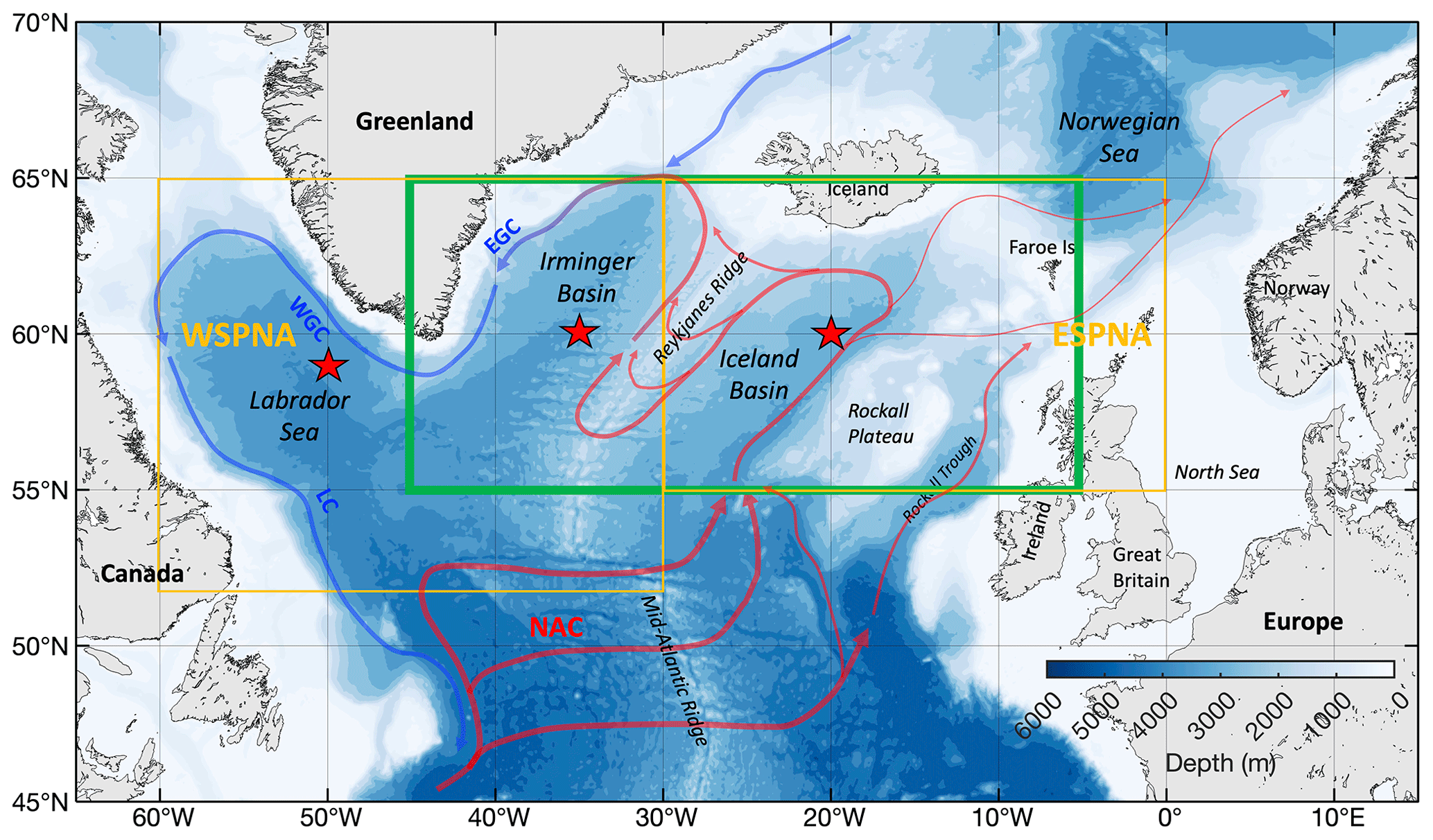
Figure 1 Bottom topography and schematic upper-ocean circulation in the subpolar North Atlantic. Abbreviations: NAC – North Atlantic Current, EGC – East Greenland Current, WGC – West Greenland Current, LC – Labrador Current. The green rectangle bounds the area used for averaging in Chafik et al. (2019). The orange rectangles bound the areas used for averaging in the western SPNA (WSPNA) and in the eastern SPNA (ESPNA). The red stars show the locations of temperature and salinity profiles shown in Fig. 17.

In this study, we focus on the subpolar North Atlantic (SPNA; Fig. 1), which is one of the key regions for deep-water formation, and as such it plays an important role in driving the AMOC. Warming, salinification, spin-down, and contraction of the North Atlantic subpolar gyre were observed in the 1990s to mid-2000s (Häkkinen and Rhines, 2004; Sarafanov et al., 2008; Holliday et al., 2008). This warming was associated with the positive phase of the Atlantic Multidecadal Oscillation (e.g., Enfield et al., 2001), partly driven by the strengthening of the North Atlantic Current (NAC) and the AMOC (Msadek et al., 2014). A cooling tendency in the SPNA started in 2006, and it ended with an exceptionally cold anomaly in 2015, termed the “cold blob” (Ruiz-Barradas et al., 2018; Chafik et al., 2019). Several studies have attributed the cold blob observed in the SPNA to the dramatic wintertime heat loss event in 2014–2015 (Josey et al., 2018; Grist et al., 2016; Duchez et al., 2016). Bryden et al. (2020), however, suggested that the cold blob could also be linked to the 2008–2009 reduction of the AMOC observed at 26.5^∘ N. Piecuch et al. (2017) showed, however, that horizontal gyre circulations provide a greater contribution to heat divergences in the SPNA than vertical overturning circulations.

Along with the cooling anomaly, a slowdown of the warm and salty NAC and redistribution of the fresher Arctic waters led to an unprecedented freshening of the SPNA in 2012–2016 (Holliday et al., 2020) that rapidly communicated with the deep waters (Chafik and Holliday, 2022). The 2013–2015 cold event in the SPNA also intensified deep-ocean convection in the Irminger and Labrador basins (de Jong and de Steur, 2016; Yashayaev and Loder, 2016). While the reduced AMOC may have influenced the intense cooling in the subpolar gyre around 2015, the resulting intensification of deep convection is expected to eventually increase the strength of the AMOC (Frajka-Williams et al., 2017). A recent analysis showed that the 2006–2015 cooling trend in the SPNA may have reversed in 2016 with a large-scale warming in the central and eastern parts of the domain due to enhanced advection of warm and saline waters from the subtropical gyre (Desbruyères et al., 2021).

Since large-scale ocean circulation is an important driver for the observed low-frequency changes in the North Atlantic, propagation of signals across the basin and between the subtropical and subpolar gyres is an intrinsic element of the variability. While westward-propagating Rossby waves and eddies provide an effective mechanism for energy transfer in the tropics and within the subtropical gyres, advection by ocean currents plays a primary role for the meridional and zonal transports along western boundary currents and at high latitudes. For example, Fu (2004) identified a propagation of the interannual sea level signal from the subtropical region to the eastern end of the Gulf Stream extension, demonstrating that the SSH variability is not just a steric response to the heat flux forcing, but also involves a dynamic response. Using a simple thermodynamic model, Dong and Kelly (2004) showed that advection by geostrophic currents can largely contribute to interannual variations of the upper-ocean heat content in the Gulf Stream region. Desbruyères et al. (2021) hypothesized that the warming signal observed in the eastern SPNA since 2016 would progressively propagate westward into the Irminger and Labrador Basins.

In areas where signal propagation is important, analyses based on the EOF decomposition may be misleading because each individual EOF pattern represents a standing oscillation. Propagating signals are often represented as a linear combination of more than one EOF pattern, such as a pair, with one mode leading the other by 90^∘ of phase in space and time (e.g., Roundy, 2015). In this case, treating consecutive EOF modes as independent physical processes is not appropriate. In this paper, we show that signal propagation is an intrinsic element of the low-frequency dynamic SSH variability in the SPNA. Therefore, the main objectives of this study are (i) to revise the definition of the North Atlantic SSH tripole by accounting for signal propagation and (ii) to explore the fidelity of the tripole in describing sea level variability in the SPNA. Nearly 30 years of quasi-global, regular satellite altimetry measurements allow us to not only resolve the interannual variability, but also gain a preliminary insight into decadal changes. Therefore, we specifically focus on interannual to decadal timescales. In addition, we discuss how the leading modes of the variability in the SPNA are related to atmospheric wind and buoyancy forcing as well as to advection by ocean currents.

2 Data

2.1 Satellite altimetry measurements

Satellite altimetry has provided accurate, nearly global, and sustained observations of sea level since the launch of the TOPEX/Poseidon mission in August 1992. We use the monthly and daily maps of SSH anomalies for the time period from January 1993 to December 2020 processed and distributed by the Copernicus Marine and Environment Monitoring Service (CMEMS; http://marine.copernicus.eu, last access: 9 March 2021). The daily maps are used only for the computation of eddy propagation velocities (Sect. 3.3). The maps are produced by the optimal interpolation of measurements from all the altimeter missions available at a given time. Prior to mapping, the along-track altimetry records are routinely corrected for instrumental noise, orbit determination error, atmospheric refraction, sea state bias, static and dynamic atmospheric pressure effects, and tides (Pujol et al., 2016). The SSH anomalies produced by CMEMS are computed with respect to a 20-year (1993–2012) mean sea surface, but we center them around the record-long mean. We also subtract the global mean sea level from SSH anomaly time series at each grid point to focus on local dynamic sea level variability not related to global changes.

2.2 Hydrographic data

To relate sea level variability to subsurface processes, we use the EN4 monthly gridded profiles of temperature and salinity (version EN.4.2.2 with mechanical/expendable bathythermograph – MBT/XBT – profile data bias adjustments from Gouretski and Reseghetti, 2010) for the period from January 1993 to December 2020 (Good et al., 2013). The profiles are based on the objective analysis of hydrographic observations (e.g., XBT, MBT, bottle, conductivity–temperature–depth – CTD, and Argo). The number of Argo profiling floats in the ocean has grown from a very sparse array of 1000 profiling floats in 2004 to a global array of more than 3000 instruments from late 2007 to the present. This means that maps in 2004–2007 and especially before 2004 are less accurate than maps in 2008–2020. The EN4 temperature and salinity profiles are used to calculate the steric SSH anomalies (SSH_ST; due to changes in density) by integrating in situ density anomalies with respect to the time mean and over the upper 1000 m, which is the depth interval occupied by the NAC. The thermosteric (SSH_T; due to temperature changes only) and halosteric (SSH_S; due to salinity changes only) contributions to SSH are calculated by integrating in situ density anomalies with respect to the time-mean values of salinity and temperature, respectively. The obtained SSH_T and SSH_S are proportional to the upper 1000 m heat and freshwater contents, respectively. Similar to the processing of altimetry data, the global mean SSH_ST, SSH_T, and SSH_S are subtracted from the respective time series at each grid point. To analyze the role of the mean ocean circulation, the individual Argo temperature and salinity profiles as well as float trajectories from the US Argo Data Assembly Center (https://www.aoml.noaa.gov/argo/#argodata, last access: 30 March 2022) are used to compute the time-mean adjusted geostrophic velocities at 1000 dbar (Schmid, 2014; see Sect. 3.3).

2.3 Atmospheric data

The observed changes in SSH are analyzed jointly with atmospheric forcing fields provided by the ERA5 climate reanalysis produced by the European Centre for Medium-Range Weather Forecasts (ECMWF) and distributed by Copernicus (https://climate.copernicus.eu/climate-reanalysis, last access: 15 December 2021). Specifically, we use the monthly averaged fields of sea level pressure (SLP), 10 m wind velocities, surface wind stress, and surface heat (shortwave and thermal radiation, sensible and latent heat fluxes) and freshwater (precipitation, evaporation) fluxes from January 1979 to December 2020 (Hersbach et al., 2019). In addition, we also use the monthly station-based NAO index based on the normalized SLP difference between Lisbon (Portugal) and Reykjavik (Iceland) from the Climate Analysis Section of the National Center for Atmospheric Research (Hurrell et al., 2003; https://climatedataguide.ucar.edu, last access: 11 March 2021).

3 Methods

To focus on interannual and longer timescales, the seasonal cycle is computed by fitting both the annual and semi-annual harmonics in a least squares sense and subtracted from all data fields and time series. The time series are further low-pass-filtered with a Lowess (locally weighted scatterplot smoothing) filter with a cutoff period of 18 months.

3.1 EOF analysis

Empirical orthogonal function (EOF) analysis is widely used to reduce the dimensionality of datasets and to extract the leading (most influential) modes of variability. Individual EOF modes, if found meaningful, are often assumed to describe different physical processes. Here, we use the conventional EOF analysis (Navarra and Simoncini, 2010) to identify the leading stationary modes of the low-frequency SSH variability in the North Atlantic. The EOF analysis is applied to both the satellite altimetry (SSH) and the EN4-derived (SSH_ST, SSH_T, and SSH_S) data. Because of the scarcity of in situ observations prior to the advent of Argo, only the EN4 data starting from 2004 were used for the EOF analysis.

For each mode j, the spatial pattern (map) is represented as a regression map (EOF_j) obtained by projecting SSH data onto the standardized (divided by standard deviation) principal component (PC_j) time series. Thus, the regression coefficients are in centimeters (local change in sea level) per 1 standard deviation change in the associated PC_j. The SSH fields can be reconstructed using a limited number of modes, N:

$$\begin{array}{}\text{(1)}& {\text{SSH}}_{\text{R}}(x,t)={\sum }_{j=\mathrm{1}}^N{\text{PC}}_j\left(t\right){\text{EOF}}_j\left(x\right),\end{array}$$

where x is the spatial position vector, and t is time. The portion of local variance explained by SSH_R (the selected number of EOF modes) is then estimated as

$$\begin{array}{}\text{(2)}& {\mathit{\sigma }}^{\mathrm{2}}\left(x\right)=\mathrm{100}\mathit{\%}\times \left[\mathrm{1}-{\displaystyle \frac{\text{var}(\text{SSH}-{\text{SSH}}_{\text{R}})}{\text{var}\left(\text{SSH}\right)}}\right].\end{array}$$

The conventional EOF analysis is not an effective method to identify propagating modes of variability. Therefore, the detection of propagating modes of the low-frequency SSH variability in the North Atlantic is carried out using the complex EOF (CEOF) analysis, which yields the spatial and temporal amplitude and phase information (Navarra and Simoncini, 2010). In essence, the CEOF analysis is based on the notion that a propagating signal should contain signals that are orthogonal to each other. In practice, the CEOF analysis of a data field is similar to the conventional EOF analysis, but applied to the field augmented in a manner such that propagating signals within it may be detected (Navarra and Simoncini, 2010). The augmentation of the data field is achieved through forming complex time series:

$$\begin{array}{}\text{(3)}& {\text{SSH}}^{\ast }\left(x,t\right)=\text{SSH}\left(x,t\right)+i\cdot {\text{SSH}}^{\text{H}}\left(xt\right),\end{array}$$

where the real part is simply the original data field (SSH) and the imaginary part is its Hilbert transform (SSH^H), representing a filtering operation upon SSH(x,t) in which the amplitude of each spectral component is unchanged but each component's phase is advanced by $\mathit{\pi }/\mathrm{2}$ (Horel, 1984). Unlike the conventional EOF analysis, the CEOF analysis yields complex eigenvectors for the spatial patterns (maps) and for their principal components (time evolution). For simplicity, henceforth, we refer to the spatial patterns as CEOFs (CEOF_j) and to the complex principal components as CPCs (CPC_j). Similar to the conventional EOF analysis, the real and imaginary parts of CEOFs are presented by regressing SSH onto the standardized real and imaginary parts of CPCs. The time–space progression of the CEOF_j mode is obtained by multiplying CEOF_j(x) and CPC_j(t) by a rotation matrix whose argument may vary between 0 and 360^∘. The real and imaginary parts of CEOFs and CPCs are also used to obtain the spatial (Φ) and temporal (θ) phases of the CEOFs.

$$\begin{array}{}\text{(4)}& \begin{array}{rl}& {\mathrm{\Phi }}_j\left(x\right)={\displaystyle \frac{\text{Imag}\left({\text{CEOF}}_j\right)}{\text{Real}\left({\text{CEOF}}_j\right)}}\\ & {\mathit{\theta }}_j\left(x\right)={\displaystyle \frac{\text{Imag}\left({\text{CPC}}_j\right)}{\text{Real}\left({\text{CPC}}_j\right)}}\end{array}\end{array}$$

3.2 Forcing mechanisms

The statistical relationship between SSH and atmospheric circulation is established by regressing SLP and 10 m wind velocity fields on PC_j and CPC₁. It is reasonable to assume that on interannual to decadal timescales the SSH changes are mostly steric (e.g., Volkov and van Aken, 2003), and therefore the mass-related changes can be neglected. The variations of SSH_ST are related to heat and freshwater fluxes as follows (e.g., Cabanes et al., 2006):

$$\begin{array}{}\text{(5)}& \begin{array}{rl}& {\partial }_t{\text{SSH}}_{\text{ST}}={\displaystyle \frac{\mathit{\alpha }}{{\mathit{\rho }}_{\mathrm{0}}{c}_{\text{p}}}}\left[Q_{\text{NET}}\left(t\right)-{\stackrel{\mathrm{‾}}{Q}}_{\text{NET}}\right]\\ & +\mathit{\beta }{S}_{\text{a}}\left[F_{\text{fw}}\left(t\right)-{\stackrel{\mathrm{‾}}{F}}_{\text{fw}}\right]+\text{Adv}\end{array},\end{array}$$

where $Q_{\text{NET}}=Q_{\text{SR}}+Q_{\text{TR}}+Q_{\text{SH}}+Q_{\text{LH}}$ is the net surface heat flux (positive into the ocean) equal to the sum of shortwave radiation (Q_SR), thermal (longwave) radiation (Q_TR), the sensible heat flux (Q_SH), and the latent heat flux (Q_LH); $F_{\text{fw}}=P-E$ is the surface freshwater flux (positive into the ocean) equal to the sum of precipitation (P) and evaporation (E); α and β are the coefficients of thermal expansion and haline contraction averaged over the upper 1000 m, respectively; ρ₀ is the reference density; c_p is the specific heat of seawater; S_a is the salinity anomaly relative to a multiyear (2004–2020) mean value averaged over the upper 1000 m; ADV denotes the SSH_ST change due to the advection of density anomalies; and the overbar indicates the climatological averages over the entire ERA5 record (1979–2020).

3.3 Ocean circulation and eddy propagation

The potential impact of oceanic advection in the SPNA is qualitatively analyzed using (i) the mean 1000 dbar velocities obtained from Argo data and (ii) eddy propagation velocities estimated from daily satellite altimetry maps, computed for the time period of 2005–2019.

The time-mean gridded adjusted geostrophic velocities at 1000 dbar are derived from Argo and altimetry using the climatological velocity field from Argo trajectories as the reference velocity following the methodology of Schmid (2014). This method uses Argo dynamic height profiles and SSH from altimetry to derive synthetic dynamic height profiles on a 0.5^∘ grid. These profiles are then used to derive the horizontal geostrophic velocities, followed by the barotropic adjustment, based on the climatology of the velocity derived from float trajectories at about 1000 dbar (the target parking depth of Argo floats). Therefore, the obtained velocities at 1000 dbar are mainly constrained by float trajectories and have very little temporal variability. Because the vertical extent of ocean eddies can reach 1000 dbar, eddies that are involved in horizontal property transports tend to follow the mean flow field at about the same depth.

To supplement the 1000 dbar velocities, we also compute eddy propagation velocities for the same time interval using a space–time lagged correlation analysis of daily SSH fields as described in Volkov et al. (2013) and Fu (2006). A velocity vector at a particular grid point is obtained as follows. First, the correlations between SSH anomalies at this grid point and at neighboring grid points are computed at various time lags. Second, the location of the maximum correlation is recorded, and a velocity vector is computed using the distance between the two grid points and the time lag. Finally, an average velocity vector weighted by correlation coefficients is computed from velocity vectors at various time lags. To obtain the results characteristic for eddy temporal and spatial scales, the time lags were limited to less than 70 d and the horizontal dimensions of the area for computing the correlations between the neighboring grid points were set to about 200 km. Because SSH is an integral quantity characteristic for the full-depth thermohaline properties, the obtained velocities are representative of property transports.

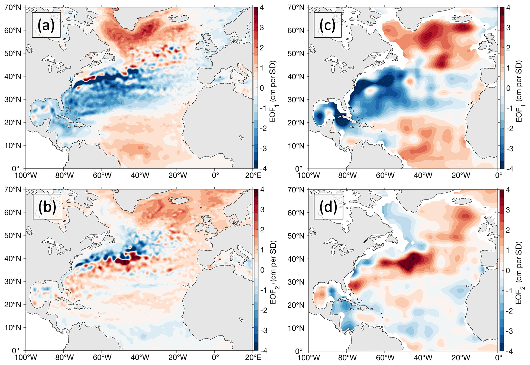
Figure 2 EOF analysis of sea level data: (a) EOF₁ and (b) EOF₂ modes of SSH anomalies measured by satellite altimetry; (c) EOF₁ and (d) EOF₂ modes of steric SSH anomalies derived from EN4 temperature and salinity profiles.

4 Results

4.1 The imprint of SSH tripole in the subpolar North Atlantic

The North Atlantic SSH tripole is defined as the leading EOF mode (EOF₁) of the low-pass-filtered dynamic SSH (Volkov et al., 2019b). It is characterized by the subtropical band (∼20^∘ N) varying out of phase with both the tropical North Atlantic (south of ∼20^∘ N) and the subpolar gyre (∼45–65^∘ N) (Fig. 2a). In 1993–2020, the tripole mode explained 27.2 % of the interannual to decadal dynamic SSH variability in the North Atlantic. The time evolution of the tripole is shown by PC₁ (solid blue curve in Fig. 3). In 1993–2010, the tripole was characterized by a general reduction of sea level in the subtropical band and a sea level rise in both the subpolar gyre and in the tropics. These tendencies reversed abruptly in 2011–2015. During the latter time interval, the subtropical gyre warmed considerably, which led to an accelerated sea level rise along the US southeastern coast with rates up to 5 times the global mean (Domingues et al., 2018; Volkov et al., 2019b), while a strong cooling occurred in the subpolar North Atlantic in 2013–2015 (Chafik et al., 2019).

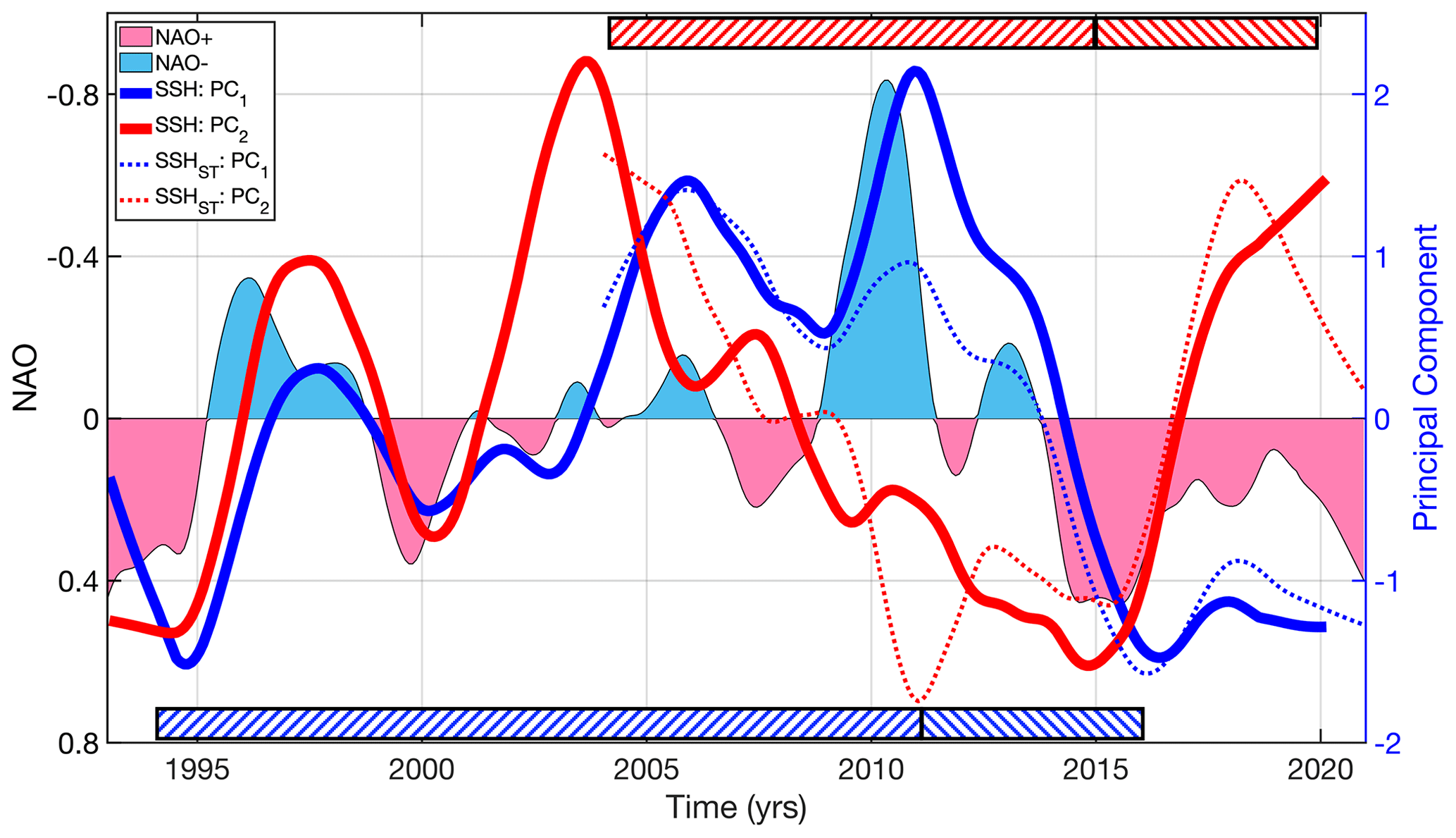
Figure 3 Time evolution (principal components) of EOF₁ (blue curves) and EOF₂ (red curves) modes of SSH (solid curves) and SSH_ST (dotted curves). The low-pass-filtered monthly NAO index is shown by color shading: (pink) positive NAO and (blue) negative NAO (note that the left axis for NAO is reversed). The horizontal bars with diagonal striped patterns indicate the time intervals used to study the relationship between sea level and surface buoyancy forcing (Sect. 4.5): 1994–2010 and 2011–2015 corresponding to the main tendencies in PC₁ (right and left tilted blue stripes, respectively), as well as 2004–2014 and 2015–2019 corresponding to the main tendencies in PC₂ (right and left tilted red stripes, respectively).

According to EOF₁ (Fig. 2a) and PC₁ (blue curve in Fig. 3), the subtropical and subpolar gyres have been in warm and cold states, respectively, since 2015. However, Desbruyères et al. (2021) reported an upper-ocean warming in the eastern SPNA that started in 2015. While this warming is apparently not part of the leading EOF mode, it appears to be consistent with the time evolution (PC₂; red curve in Fig. 3) of the second EOF mode (EOF₂; Fig. 2b). The EOF₂ mode explains 13.4 % of the variance and exhibits a pattern that suggests changes in the strength and likely meridional shifts of the Gulf Stream to the east of Cape Hatteras. This mode is also responsible for decadal changes in the eastern and northeastern SPNA: a generally positive SSH tendency in 1993–2003, an SSH decrease in 2004–2014, and an SSH increase since 2015 (red curve in Fig. 3), consistent with the observations of Desbruyères et al. (2021).

Sea level changes associated with EOF₁ and EOF₂ are mostly steric, i.e., determined by density variations. This is confirmed by the spatial structures (Fig. 2c, d) and temporal evolutions (PCs; dotted curves in Fig. 3) of EOF₁ and EOF₂ of the low-pass-filtered SSH_ST accounting for 45.2 % and 16.8 % of the variance, respectively. These two leading modes are similar to those of the low-pass-filtered SSH (Fig. 2a, b; solid curves in Fig. 3). The correlation between PC₁ of SSH and PC₁ of SSH_ST is 0.94, and the correlation between PC₂ of SSH and PC₂ of SSH_ST is 0.88, which is significant at 95 % confidence. Furthermore, the steric sea level changes are governed by changes in the upper 1000 m ocean heat content. The spatial patterns and the signs of EOF₁ and EOF₂ of the low-pass-filtered SSH_ST are determined by the thermosteric sea level variability; the EOF₁ and EOF₂ of the low-pass-filtered SSH_T are nearly identical to the EOF₁ and EOF₂ of the low-pass-filtered SSH_ST (compare Figs. 4a, b and 2c, d). The correlation between the PC₁ of SSH_ST and SSH_T is 0.99, and the correlation between the PC₂ of SSH_ST and SSH_T is 0.97 (Fig. 4c). The thermosteric sea level changes are partly compensated for by the halosteric sea level changes because the warmer (colder) water is usually saltier (fresher). Indeed, the EOF₁–PC₁ and EOF₂–PC₂ of SSH_S (Fig. 4d–f) generally offset those of SSH_T (Fig. 4a–c). For example, the cooling tendencies observed in the SPNA in 2006–2016 depicted by EOF₁ and in 2004–2011 depicted by EOF₂ were associated with respective upper-ocean freshening.

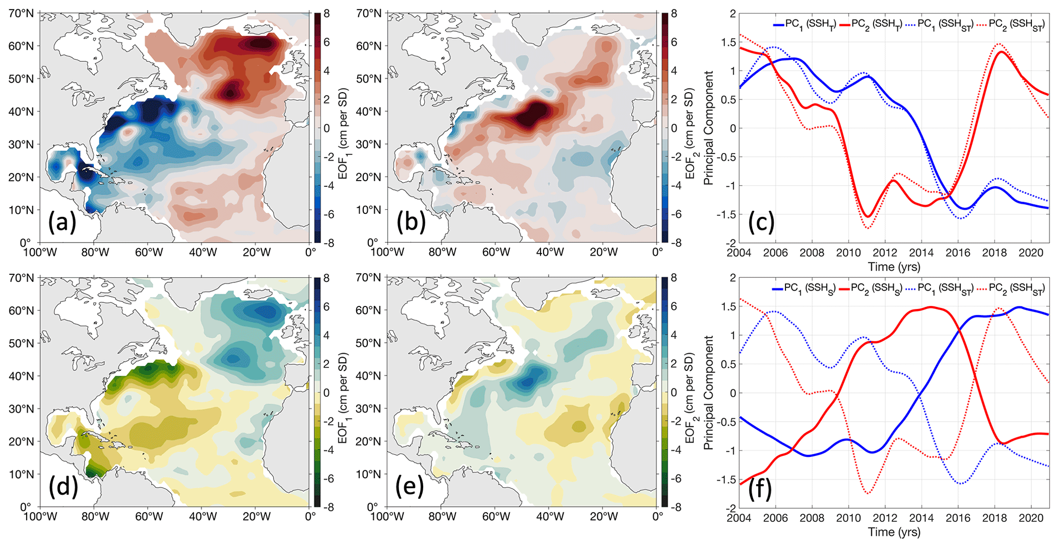
Figure 4 EOF analysis of thermosteric (SSH_T) and halosteric (SSH_S) sea level derived from EN4 temperature and salinity profiles: (a) EOF₁ and (b) EOF₂ modes of SSH_T, (c) PC₁ (blue) and PC₂ (red) of SSH_ST (dotted) and SSH_T (solid), (d) EOF₁ and (e) EOF₂ modes of SSH_S, (f) PC₁ (blue) and PC₂ (red) of SSH_ST (dotted) and SSH_S (solid).

The percentage of the local SSH variance explained by the two leading EOF modes in the SPNA exhibits the following patterns. The North Atlantic SSH tripole, characterized by the EOF₁–PC₁ of the low-pass-filtered SSH, explains the majority (60 %–90 %) of the interannual SSH variance in the Labrador Sea and in the Irminger Basin (western SPNA; Fig. 5a). The EOF₂ mode explains a substantial amount of the interannual SSH variance (60 %–80 %) in the northeastern SPNA east of Greenland (Fig. 5b). The two leading modes together (EOF₁ + EOF₂; Fig. 5c) explain most of the interannual SSH variability in the SPNA north of 52^∘ N, except the southern part of the Iceland Basin and the Rockall Trough, where the eddy variability associated with the NAC branches is relatively strong. It is interesting to note that while the EOF₁ depicts the interannual SSH variability over the deep parts of the Labrador Sea and Irminger Basin, the EOF₂ depicts the interannual SSH variability over the shallower waters of the Rockall Plateau, parts of European continental shelf and slope, Reykjanes Ridge, Iceland shelf, and along the Irminger and East Greenland Currents.

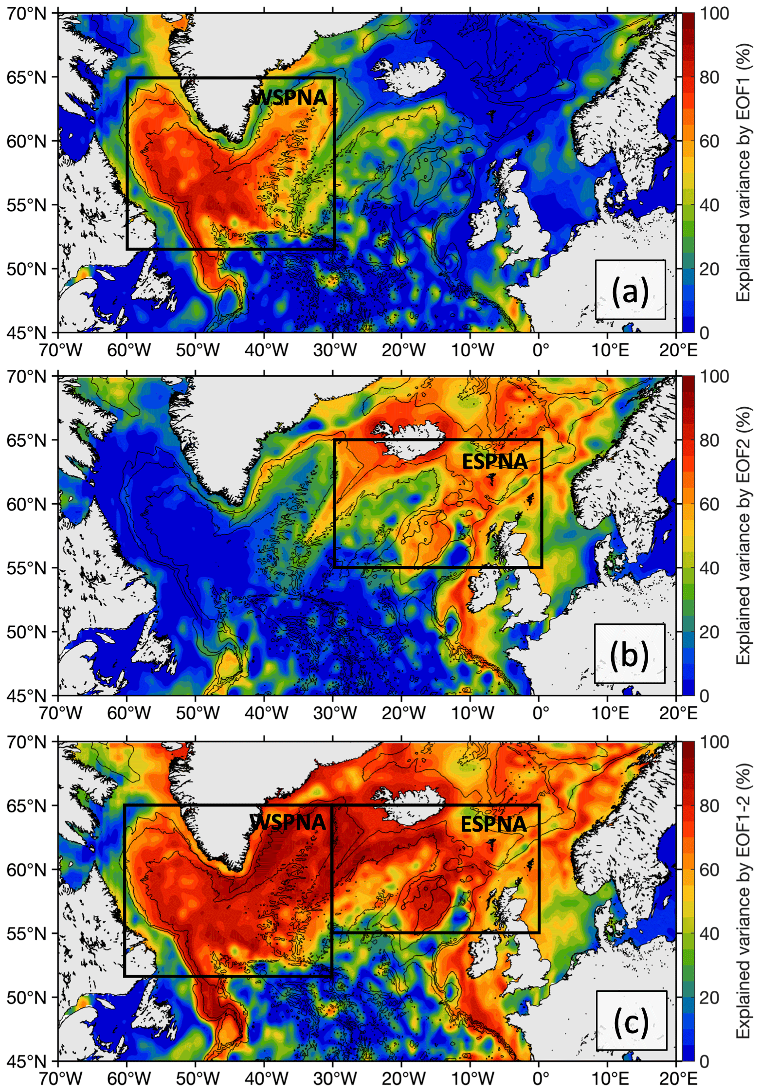
Figure 5 The portion of local variance of the low-pass-filtered SSH explained by (a) EOF₁, (b) EOF₂, and (c) the composition of EOF₁ and EOF₂ in the subpolar gyre of the North Atlantic. The bathymetry contours are shown every 1000 m. The rectangles bound the areas of the western SPNA (WSPNA) and eastern SPNA (ESPNA) used for averaging the time series shown in Fig. 7.

4.2 Interannual SSH variability in the subpolar North Atlantic

Chafik et al. (2019) discussed the variability of dynamic SSH in 1993–2016 averaged over 5–45^∘ W and 55–65^∘ N in the SPNA (green rectangle in Fig. 1). Here, we present both the updated SSH time series (black curve in Fig. 6) and the SSH_R time series reconstructed with EOF₁ (blue curve in Fig. 6) and EOF₂ (red curve in Fig. 6), averaged over the same region. When disregarding shorter-term, year-to-year variations, SSH increased by about 6 cm in 1993–2005, decreased by the same amount in 2006–2015, and then increased again by about 5 cm in 2016–2020. As the SSH_R time series show, neither the EOF₁ nor the EOF₂ alone can adequately explain the SSH variability in the SPNA. However, their sum (dotted curve in Fig. 6) is sufficient to reasonably reconstruct SSH in the region. The SSH_R computed with the two leading EOFs matches the observed SSH well, with a correlation of 0.96, meaning that SSH_R explains about 92 % of the SSH variance. Individually, the EOF₁ and EOF₂ modes explain 44 % and 48 % of the SSH variance, respectively.

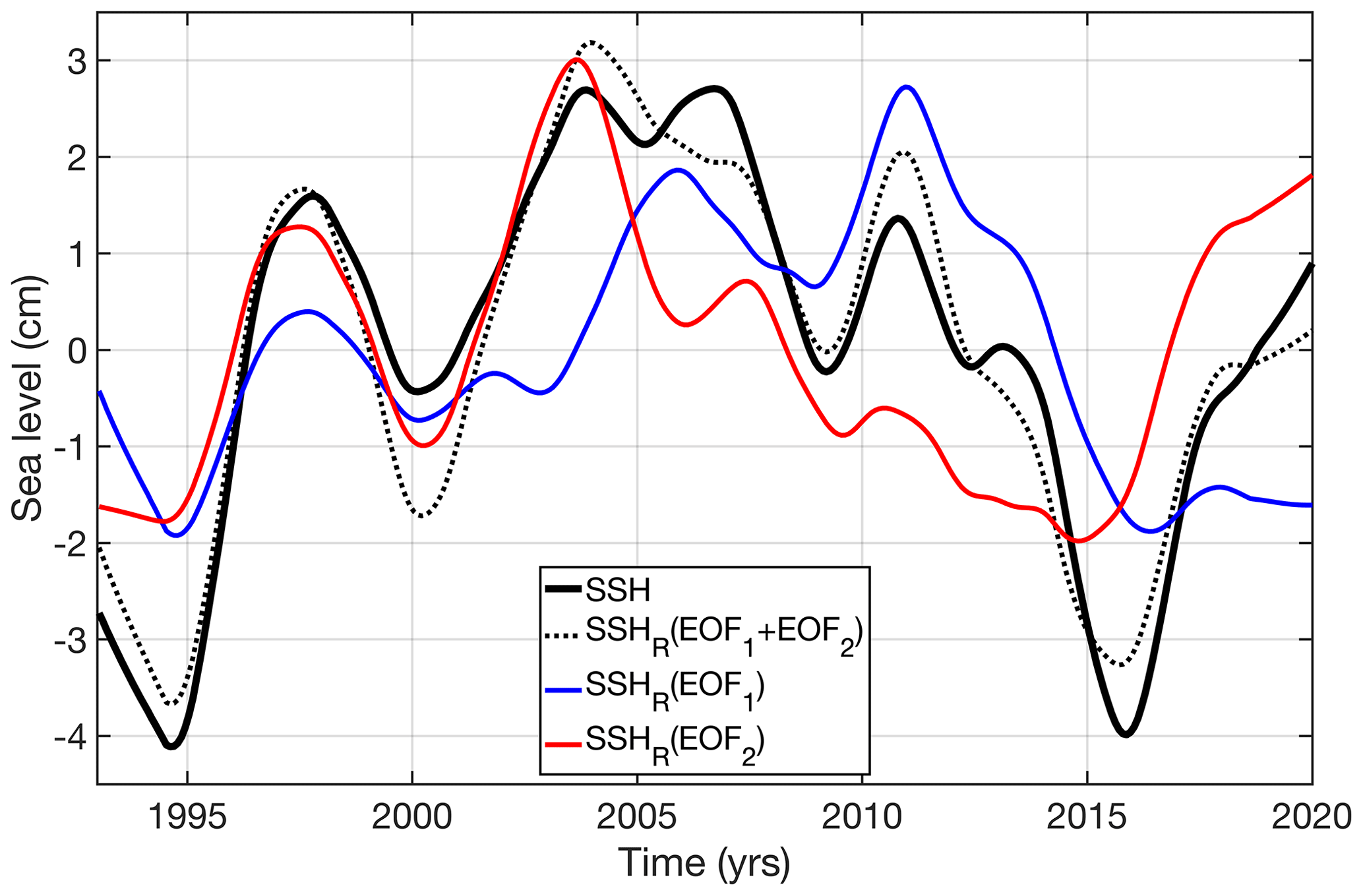
Figure 6 Time series averaged over 5–45^∘ W and 55–65^∘ N (as in Chafik et al., 2019): detrended SSH (solid black), SSH_R reconstructed using the combination of EOF₁ and EOF₂ (dotted black), SSH_R reconstructed using EOF₁ (blue), and SSH_R reconstructed using EOF₂ (red).

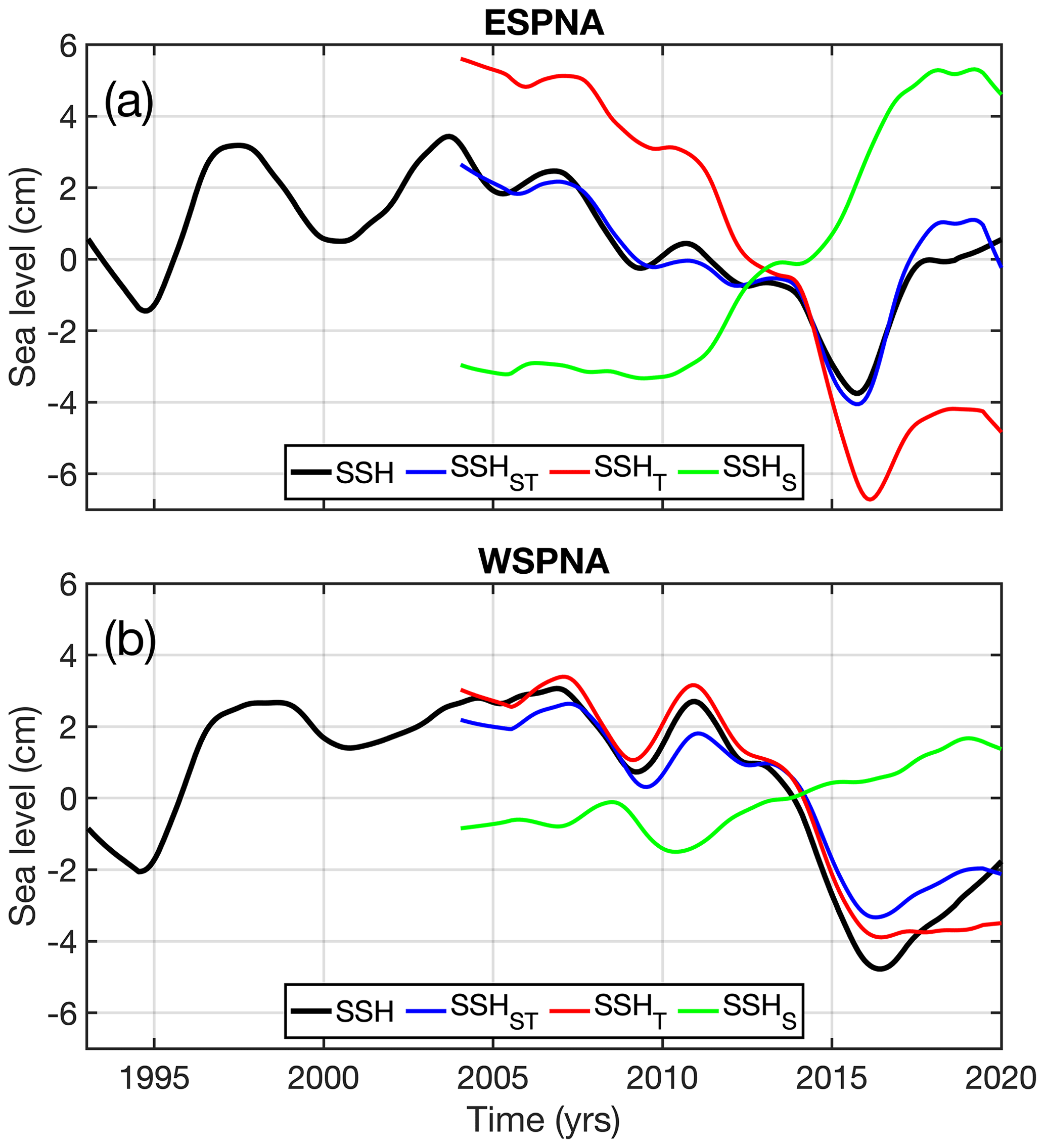
Figure 7 Time series of SSH (black), SSH_ST (blue), SSH_T (red), and SSH_S (green) averaged over (a) 0–30^∘ W and 55–65^∘ N in the eastern SPNA (ESPNA) and (b) 30–60^∘ W and 53–65^∘ N in the western SPNA (WSPNA) (the areas of ESPNA and WSPNA are shown in Figs. 1 and 5).

In order to illustrate the relative contribution of temperature and salinity changes to the interannual to decadal variability of SSH in the SPNA, we compute the averages of SSH_ST, SSH_T, and SSH_S over two regions (outlined by orange rectangles in Fig. 1): (i) the eastern SPNA (0–30^∘ W and 55–65^∘ N), including the Iceland Basin, Rockall Plateau, and the Rockall Trough (Fig. 7a); and (ii) the western SPNA (30–60^∘ W and 53–65^∘ N), including the Irminger Basin and the Labrador Sea (Fig. 7b). The time series of SSH_ST closely matches those of SSH, with the correlation between them above 0.95 and the root mean squared differences of 0.4 in the eastern SPNA and 0.8 cm in the western SPNA (compare black and blue curves in Fig. 7). This means that the variability of SSH in the SPNA is mostly steric in nature. The remaining difference between SSH and SSH_ST can be attributed to density changes at depths greater than 1000 m and to errors in data; the contribution of barotropic signals is expected to be small at the timescales considered. In 2005–2015, SSH_ST decreased by about 6 cm in the eastern SPNA and 5 cm in the western SPNA (blue curves in Fig. 7). The decrease in SSH_ST was caused by cooling and the associated reduction of SSH_T by about 12 cm in the eastern SPNA and 6 cm in the western SPNA (red curves in Fig. 7). The reduction of SSH_T in both the eastern SPNA and western SPNA was compensated for by a freshening-induced increase in SSH_S by about 5 and 1 cm, respectively (green curves in Fig. 7). It is interesting to note that while the sign of SSH_ST anomalies is determined by SSH_T, the contribution of SSH_S is substantial and comparable to the contribution of SSH_T, especially in the eastern SPNA.

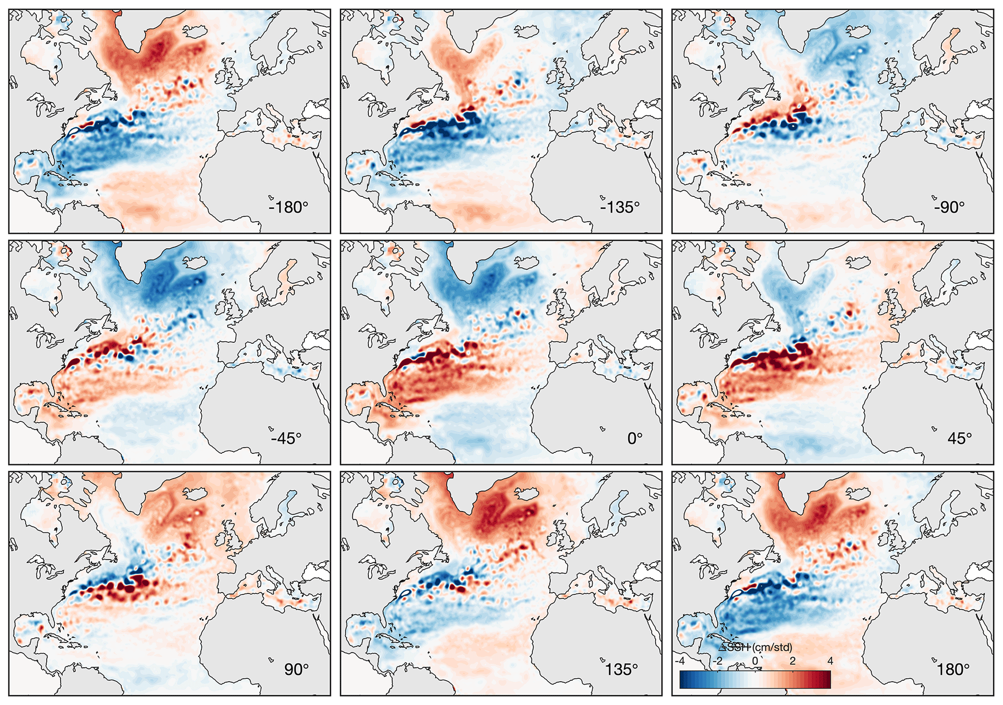
Figure 8 Reconstruction of the CEOF₁ mode of the low-pass-filtered SSH anomalies showing one full cycle (−180–180^∘) at 45^∘ phase intervals. The angle of rotation is shown in the right lower corner of each panel. Note that CEOF₁ rotated at 180 and 90^∘ is similar to EOF₁ and EOF₂, respectively.

4.3 Propagation of SSH anomalies

We have shown that SSH in the SPNA is adequately reconstructed by the two leading EOF modes. If the observed phase difference between these statistical modes is due to signal propagation, then both EOF₁ and EOF₂ describe the same physical process at different stages of its evolution. Indeed, the application of the CEOF analysis presented below shows that EOF₁ and EOF₂ resemble the real and imaginary parts of CEOF₁, respectively. Recall that the real and imaginary parts of CEOF_j can be interpreted as the propagating signal at two stages separated by a quarter-cycle. Displayed in Fig. 8 is the time evolution of the spatial pattern of SSH reconstructed with CEOF₁ mode for one full cycle at phase stages separated by 45^∘. Note that SSH patterns at phases ±180 and 90^∘ are almost identical to EOF₁ and EOF₂, respectively (Fig. 2a, b). Likewise, illustrating the temporal evolution of the CEOF₁ mode, the real part of CPC₁ when rotated by 180^∘ (Fig. 9, dashed blue curve) corresponds to PC₁ (Fig. 3, blue curve) and the imaginary part of the CPC₁ (Fig. 9, red curve) corresponds to PC₂ (Fig. 3, red curve).

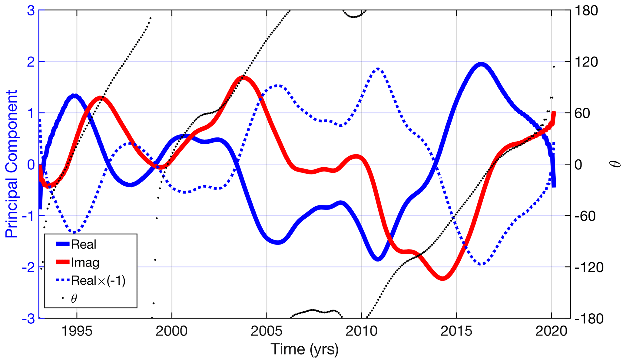
Figure 9 Time evolution of the CEOF₁ mode: (solid blue curve) real and (red curve) imaginary components, (dashed blue curve) real part of CPC₁ rotated by 180^∘, and (dotted black curve) the temporal phase of the mode.

The reconstruction of the CEOF₁ mode (Fig. 8) shows that the tripole-related sea level variations in the tropical and subtropical bands resemble a standing wave. Negative and positive SSHs in the tropical and subtropical bands at phase 0^∘ are gradually replaced by positive and negative SSHs at phase 180^∘, respectively, without a notable sign of signal propagation. On the other hand, a signal propagation is evident in the subpolar band of the tripole. In the first half of the cycle at phases −180 and −135^∘, negative anomalies start emerging near the eastern boundary, when positive anomalies are mainly concentrated in the Irminger Basin and Labrador Sea. As the negative anomalies propagate towards the Irminger Basin and the Labrador Sea, the positive anomalies extend south-southwestward along the North American east coast and eventually leak into the subtropical gyre. SSH anomalies in the subtropical gyre then switch sign from negative to positive, which ultimately leads to the emergence of small positive SSH anomalies along the European coast seen at phase 0^∘. These anomalies are intensified at phase 45^∘ and propagate westward, peaking in the Iceland Basin at phase 135^∘, in the Irminger Basin at phase 135–180^∘, and in the Labrador Sea at phase 180^∘, completing the full cycle.

As demonstrated by the real and imaginary CPC₁ time series (blue and red curves in Fig. 9, respectively) and the temporal phase (dotted black curve in Fig. 9), there were almost three full cycles of the decadal gyre-scale sea level changes that exhibited signal propagation in the SPNA in 1993–2020. One full cycle is associated with the temporal phase change from −180 to 180^∘. In the northeastern SPNA, the first cycle started with a low SSH in 1993 (red curve), and it progressively reached high SSH in 1996, corresponding to phases −90 and 90^∘ in Fig. 8, respectively. This signal propagated westward, with SSH reaching maximum values in the Irminger Basin and Labrador Sea in 1998 (dashed blue curve), corresponding to phase 180^∘ in Fig. 8. Counting from the first SSH minimum in the northeastern SPNA in 1993 (red curve) to the second SSH minimum in the western SPNA in 2000–2001 (dashed blue curve), the first cycle lasted 7–8 years. The second cycle started with a low SSH in the northeastern SPNA in 1999 (second minimum in the red curve) and ended with a local (third) SSH minimum in 2008–2009 in the western SPNA (dashed blue curve), thus taking 9–10 years to complete. Based on the temporal phase of the CPC₁ (dotted black line in Fig. 9), there was no apparent propagation in 2006–2009. The third cycle can be counted from a local (third) SSH maximum in the northeastern SPNA in 2009 (red curve) that reached the Labrador Sea in 2011 (dashed blue curve). The second SSH maximum of this cycle was not yet reached by the end of the record in 2020, so its overall duration has exceeded 10 years.

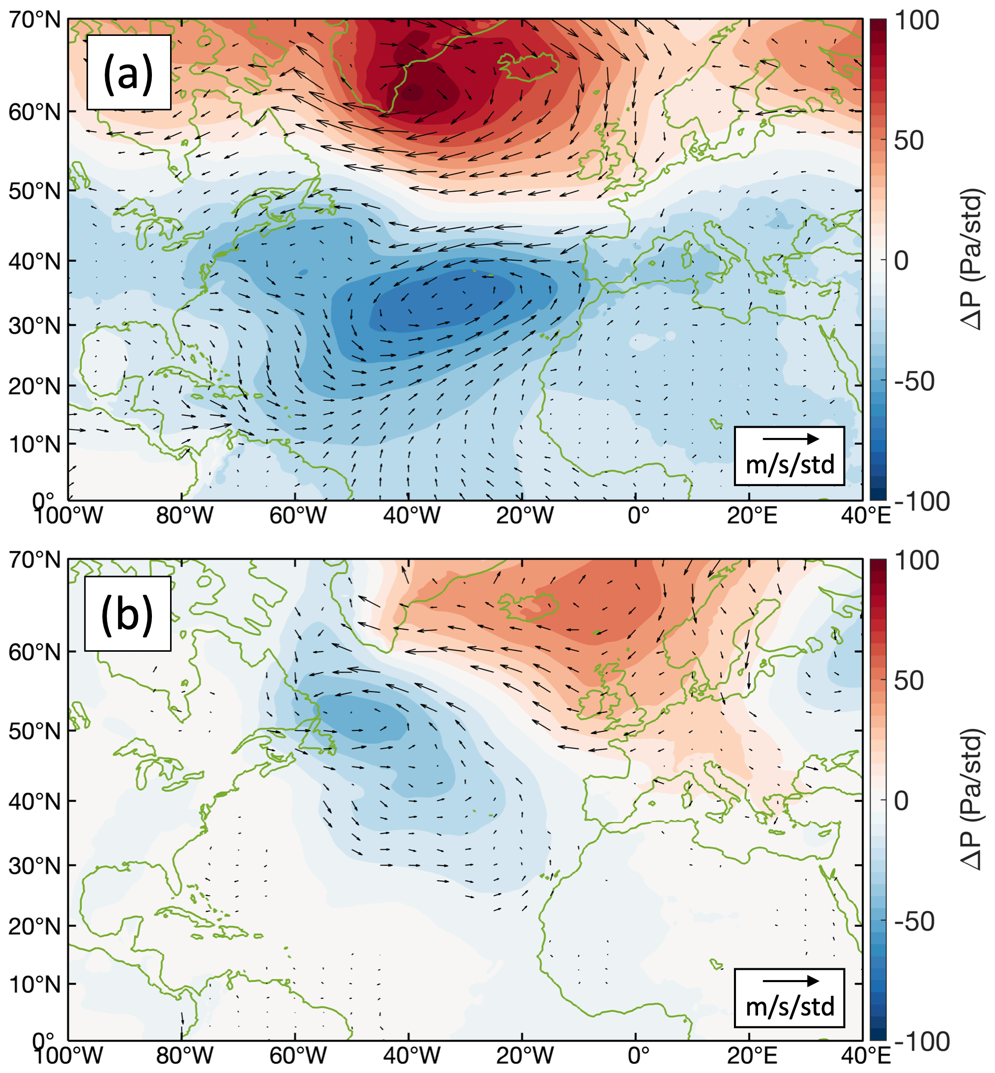
Figure 10 Regression maps of (color) SLP and (arrows) 10 m wind velocity on (a) PC₁ and (b) PC₂; the units are Pa per standard deviation of PC_j and m s⁻¹ per standard deviation of PC_j, respectively. Arrows are plotted only at locations where regression coefficients are significant at 95 % confidence.

4.4 Relationship between sea level and wind forcing

The maximum correlation between the PC₁ (solid blue curve in Fig. 3), showing the time evolution of the North Atlantic SSH tripole, and the low-pass-filtered NAO index (shaded area in Fig. 3) is −0.73, with the NAO leading by 10 months (the 95 % significance level for correlation is about 0.45). The lag probably indicates the oceanic adjustment time to a variable wind forcing. Regression of SLP and 10 m winds on the PC₁ displays a familiar NAO dipole pattern with a cyclonic (negative) anomaly in the subtropical high and an anticyclonic (positive) anomaly in the subpolar low SLP centers (Fig. 10a). The weaker (stronger) subtropical high and subpolar low associated with weaker (stronger) westerly winds in the midlatitude North Atlantic lead to lower (higher) sea levels in the subtropical North Atlantic and higher (lower) sea levels in the SPNA.

Interestingly, while correlation between the PC₂ and the NAO is not significant, regression of SLP and 10 m winds on the PC₂ (Fig. 10b) also exhibits a dipole pattern similar to the NAO, but with somewhat shifted pressure centers. This suggests that both the EOF₁ and the EOF₂ of the low-pass-filtered SSH are possibly driven by the same atmospheric process but are associated with different phases of its evolution or different regimes. To support this argument, we also regressed SLP and 10 m winds on the real parts of CPC₁ rotated every 45^∘ at ±180^∘, thus yielding the full-cycle evolution of wind forcing patterns associated with the leading CEOF mode (Fig. 11). The obtained patterns illustrate that the distribution of SLP and 10 m wind anomalies, as the subtropical high and the subpolar low centers change their position and intensity, is clearly related to the SSH patterns associated with the CEOF₁ (compare Figs. 8 and 11). The positive (negative) SLP and anticyclonic (cyclonic) wind anomalies drive the near-surface Ekman convergence (divergence) and lead to the upper-ocean warming (cooling) and, consequently, higher (lower) sea levels. It should be noted that the SLP and wind anomaly patterns associated with PC₁ and PC₂ (Fig. 10) are identical to wind forcing patterns associated with CPC₁ at phases ±180 and 90^∘ (or at phases 90 and 0^∘ if the sign is reversed) (Fig. 11).

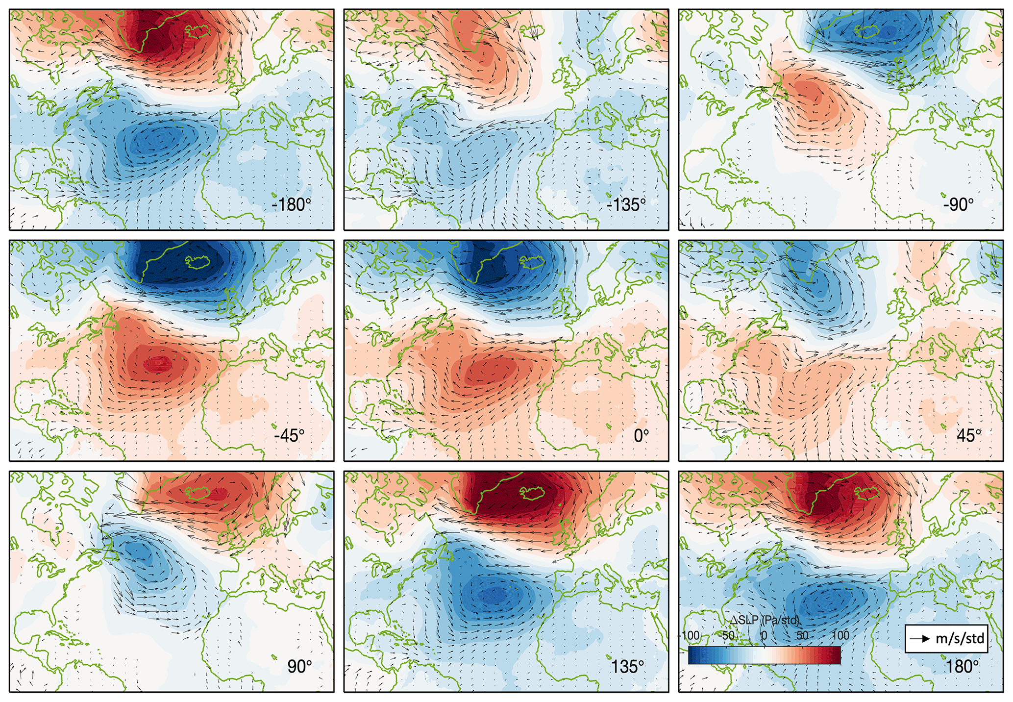
Figure 11 Regression maps of (color) sea level pressure (SLP) and (arrows) 10 m wind velocity on CPC₁ rotated every 45^∘ at ±180^∘ showing the full-cycle evolution of wind forcing patterns associated with the CEOF₁ mode of the low-pass-filtered SSH. Arrows are plotted only at locations where regression coefficients are significant at 95 % confidence.

The westward propagation of negative (positive) SSH from the northwest European shelf towards the Labrador Sea clearly follows similar shifts in the position of SLP and wind anomalies. Indeed, the center of the positive (anticyclonic) SLP anomaly associated with EOF₂ or with CEOF₁ at phase 90^∘ is located near eastern Iceland, and the anticyclonic atmospheric circulation pattern covers the area of positive SSH anomalies in the eastern–northeastern part of the SPNA (compare Figs. 10b, 11, and 2b). The positive SLP anomaly pattern then intensifies and shifts westward towards the eastern coast of Greenland (Figs. 10a and 11 at phases 135 and 180^∘). This shift corresponds to the observed propagation of SSH anomalies towards the Irminger Basin and the Labrador Sea (Fig. 11 at phases 90, 135, and 180^∘). The established statistical relationship suggests that SSH and the upper-ocean heat content anomalies in the SPNA result from the oceanic adjustment to persistent wind forcing lasting longer than a year. On the other hand, we acknowledge that oceanic feedback to atmospheric forcing is also possible on these timescales.

The analysis presented here indicates that the NAO, which is correlated with the PC₁ only, is not a sufficient proxy for wind forcing over the SPNA. This is mostly because the definition of the NAO is limited by an assumption that it is a standing oscillation pattern with the fixed subtropical high-pressure and the subpolar low-pressure centers. We have shown that the observed propagation of the dynamic SSH anomalies in the SPNA is linked to the NAO-like atmospheric pressure and wind patterns that change their location and intensity. The importance of accounting for the position and intensity of an atmospheric center of action for determining causal relationships within the coupled ocean–atmosphere system in the North Atlantic has been reported earlier (e.g., Hameed and Piontkovski, 2004; Hameed et al., 2021). Our results provide further evidence that the attribution of oceanic signals to the conventional NAO index, which generalizes and often oversimplifies the atmospheric variability, is not always appropriate.

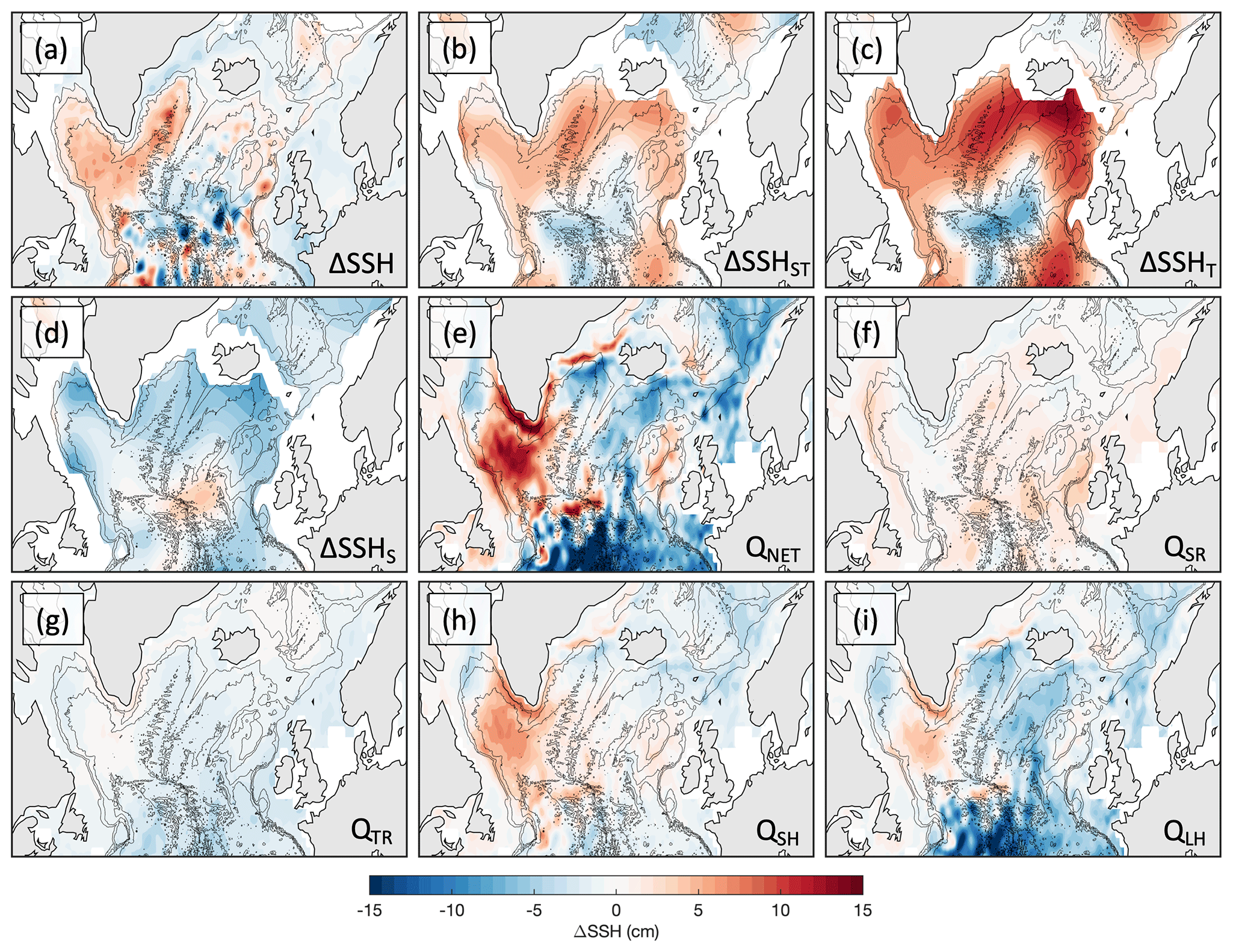
Figure 12 SSH change in 1994–2010: (a) total as observed with satellite altimetry (ΔSSH); (b) steric (ΔSSH_ST), (c) thermosteric (ΔSSH_T), and (d) halosteric (ΔSSH_S) as estimated from EN4 data; (e) due to the net surface heat flux (Q_NET), (f) due to the shortwave radiation (Q_SR), (g) due to the thermal (longwave) radiation (Q_TR), (h) due to the sensible heat flux (Q_SH), and (i) due to the latent heat flux (Q_LH) as provided by the ERA5 reanalysis.

4.5 Relationship between sea level and surface buoyancy forcing

To investigate the impact of surface buoyancy forcing on the interannual to decadal changes in SSH, we select four time intervals characteristic of the main tendencies reflected by PC₁ and PC₂ in Fig. 3 (by the real and imaginary CPC₁ in Fig. 9): 1994–2010 and 2011–2015 for PC₁ (real CPC₁) and 2004–2014 and 2015–2019 for PC₂ (imaginary CPC₁). Because the two leading modes of variability have quite distinct spatial footprints, we can better assess and visualize the role of buoyancy forcing in driving each mode. For the selected time intervals, we present the absolute changes in SSH, SSH_ST, SSH_T, and SSH_S (Figs. 12–15a–d) and the contributions to these changes driven by surface heat (Figs. 12–15e–i) in chronological order. Because the SSH changes driven by surface freshwater fluxes (P+E) appear to be 3 orders of magnitude smaller than those driven by surface heat fluxes, they are not considered in the following. The impact of surface freshwater fluxes on the regional SSH_S changes (Figs. 12–15d) is also negligible, thus suggesting that these changes are mainly driven by the advection of freshwater.

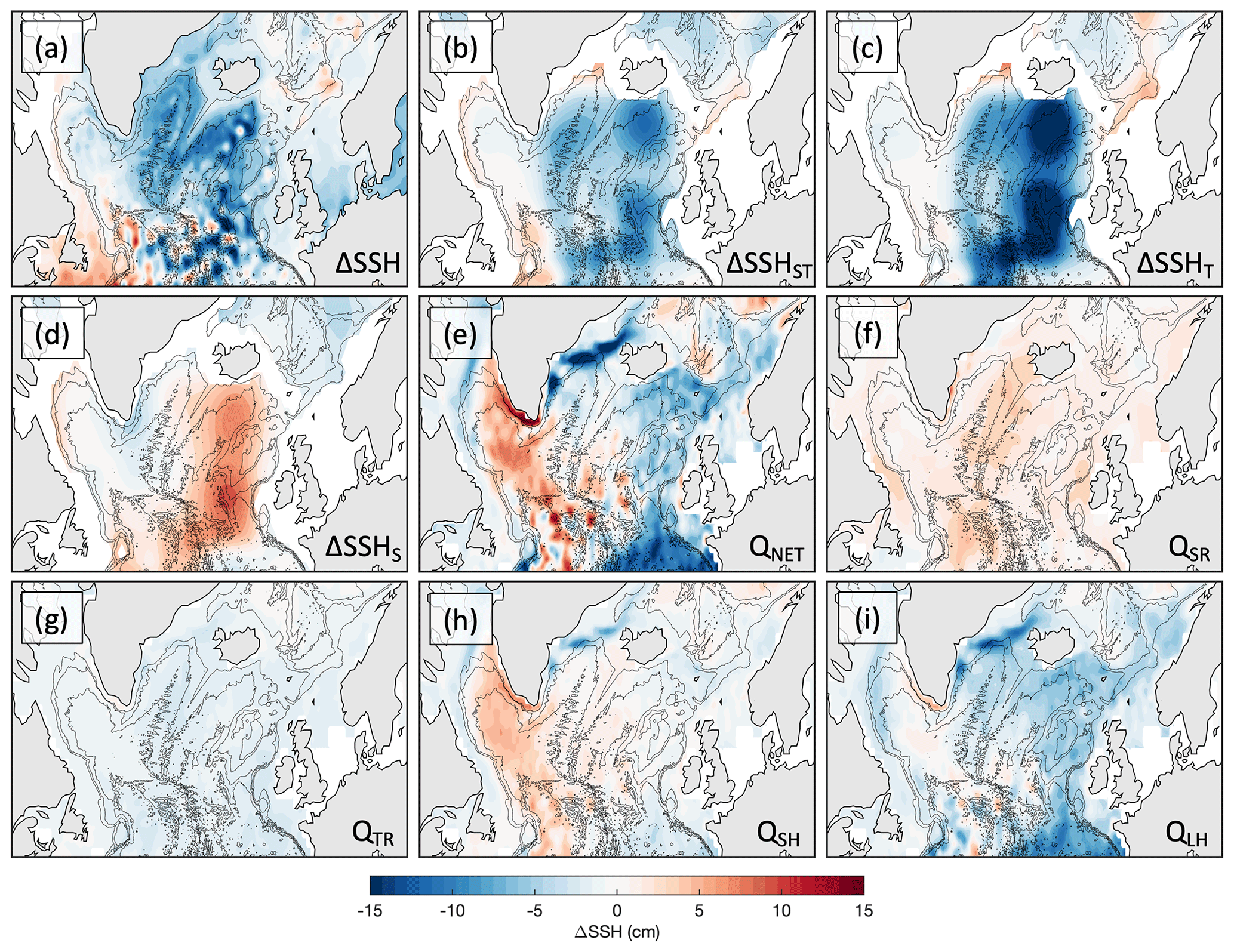
Figure 13 Same as Fig. 12 but for the 2004–2014 period.

The overall increase in sea level in the Labrador Sea and Irminger Basin in 1994–2010 associated with the North Atlantic SSH tripole and depicted by the PC₁ (blue curve in Fig. 3) and the real part of CPC₁ (dotted blue curve in Fig. 9) is well explained by the SSH_ST change (Fig. 12a, b). The SSH_ST change exceeds the total SSH change only over the northern part of the Iceland Basin and over the Rockall Plateau and Rockall Trough. The differences between the changes of SSH and SSH_ST in 1994–2010 can be due to the lack of in situ temperature measurements prior to the start of the widespread use of Argo floats in the region. The spatial pattern and the sign of the observed SSH_ST change are determined by the SSH_T change (Fig. 12c), which is partly balanced by the SSH_S change (Fig. 12d). The net surface heat flux anomalies (Q_NET) can explain the SSH–SSH_ST increase in the Labrador Sea and over the Rockall Plateau and the SSH–SSH_ST decrease in the southern part of the Iceland Basin (Fig. 12e). The shortwave (Q_SR) and thermal (Q_TR) radiation anomalies largely compensated for each other (Fig. 12f, g), and the largest contribution to Q_NET anomalies in 1994–2010 came from the sensible (Q_SH) and latent (Q_LH) heat flux anomalies. The observed warming in the Labrador Sea in 1994–2010 was mainly caused by the Q_SH anomaly. This implies that there were tendencies for the ocean to be colder than the air aloft and for the air temperature just above the surface to be increasing upward. This pattern is typical during periods with an anomalous heat flux into the ocean (positive Q_SH anomaly). The secondary contribution to the Labrador Sea warming came from the positive Q_LH anomaly, also suggesting that the air temperature was higher than the ocean temperature and the humidity was sufficient to cause condensation of water vapor on the surface of the ocean. This resulted in a loss of heat from air into the ocean (positive Q_LH anomaly). In the northern part of the Irminger Basin, the increase in SSH–SSH_ST in 1994–2010 (Fig. 12a, b) was associated with the concurrent heat loss to the atmosphere (Fig. 12e), which must have been compensated for by increased oceanic heat advection into the region.

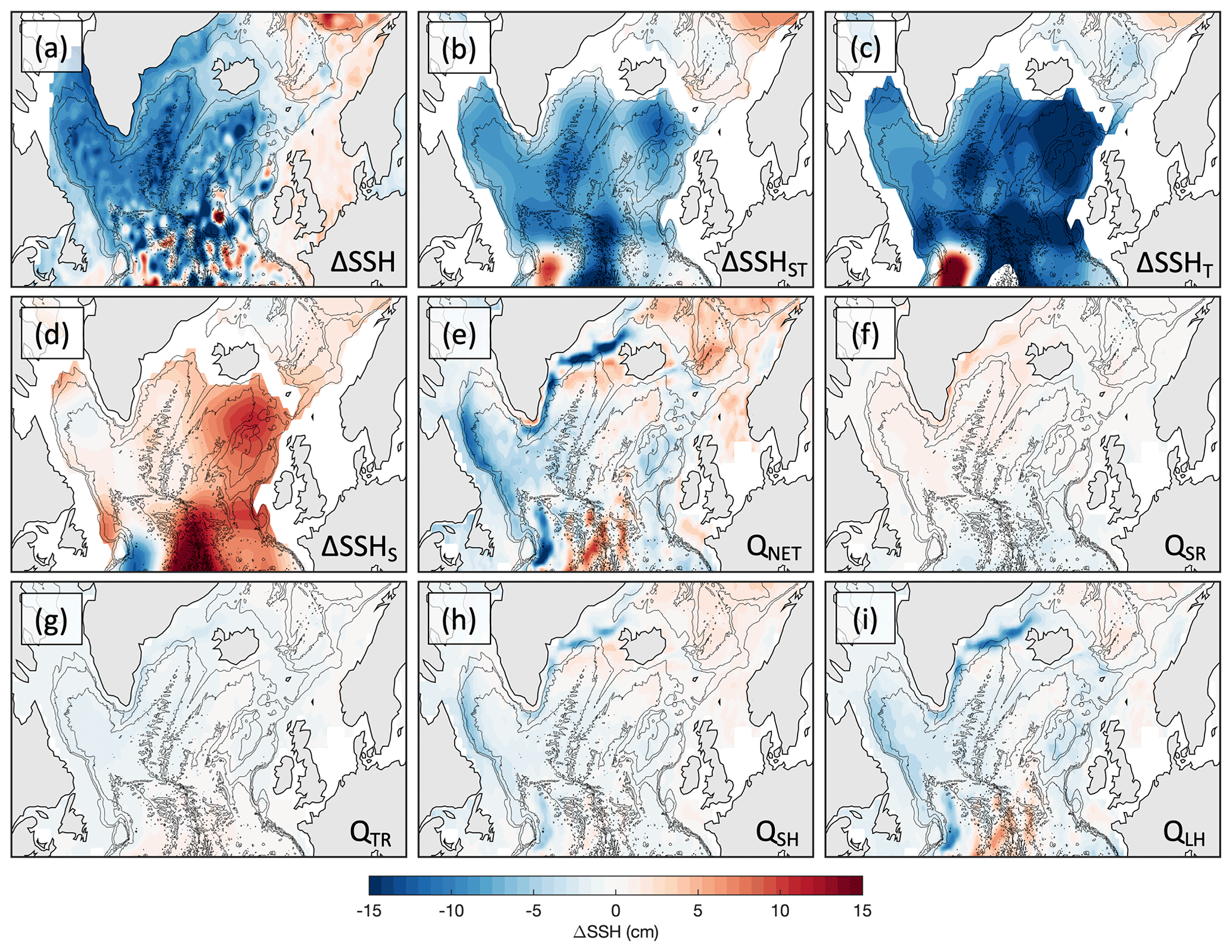
Figure 14 Same as Fig. 12 but for the 2011–2015 period.

The 2004–2014 period, depicted by the PC₂ (red curve in Fig. 3) and the imaginary part of CPC₁ (red curve in Fig. 9), was characterized by a decade-long decrease in SSH over most parts of the northeastern SPNA (Fig. 2b, solid red curves in Figs. 3 and 9), in particular in the Iceland and Irminger basins (Fig. 13a). This decrease observed by satellite altimetry corresponds well to the decrease in SSH_ST (Fig. 13b), which was mainly determined by ocean cooling reflected in the SSH_T change (Fig. 13c). The latter was partly compensated for by a freshening-induced SSH_S increase in the eastern SPNA (Fig. 13d). The Q_NET anomaly (Fig. 13e) can explain the 2004–2014 cooling and SSH decrease only in the eastern–northeastern SPNA. In the interior of the Labrador Sea, while the SSH was decreasing, the atmosphere was warming the ocean (Fig. 13e), which implies an increased oceanic heat transport out of the basin. The contributions of Q_SR and Q_TR anomalies to the Q_NET anomaly are rather small and compensate for each other (Fig. 13f, g). It is interesting to note that unlike during the 1994–2010 period (Fig. 12f, g) the contributions of Q_SH and Q_LH anomalies are geographically distinct (Fig. 13f, g). The Q_SH anomaly makes the largest contribution to the positive Q_NET anomaly in the western SPNA (Fig. 13h), meaning that in this region the ocean temperature relative to the air temperature was colder than usual. This led to an anomalous heat flux from the atmosphere into the ocean. In contrast, in the eastern–northeastern SPNA, the Q_LH anomaly was the largest contributor to the negative Q_NET anomaly (Fig. 13i). In the latter case, the ocean temperature relative to the air was warmer than usual, thus favoring evaporation and the associated upper-ocean cooling.

In 2011–2015, a tripole-related decrease in SSH (PC1 and the real part of CPC1 in Figs. 3 and 9) occurred over most parts of the SPNA, with the largest anomalies in the Irminger Basin and the Labrador Sea (Fig. 14a). This decrease was mainly steric in nature (Fig. 14b), and it was associated with strong cooling (Fig. 14c) and freshening (Fig. 14d). It is interesting to note that in most regions the Q_NET anomaly did not provide the largest contribution to the observed SSH change in 2011–2015 (Fig. 14d). Only its contributions over the northwest European shelf, in the Norwegian Sea, and along the East Greenland and Labrador Currents were substantial. This means that the oceanic advection of heat and freshwater was the major driver for the 2011–2015 decrease in SSH in most parts of the SPNA. The distributions of ΔSSH_T (Fig. 14c) and ΔSSH_S (Fig. 14d) suggest that advection was mainly associated with the NAC. The structure of the Q_NET anomalies was mostly determined by the nearly equal contributions from Q_SH and Q_LH anomalies, with the strongest impacts along the East Greenland and Labrador Currents (Fig. 14h, i). The Q_SR and Q_TR anomalies were somewhat smaller and largely compensated for each other (Fig. 14f, g). We recall that an exceptionally cold anomaly, termed the cold blob, occurred in the SPNA in 2015 (Ruiz-Barradas et al., 2018; Chafik et al., 2019). The analysis presented here shows that while the onset of this strong cooling started in 2004 in the eastern SPNA (red curve in Fig. 7a) and was partly driven by the negative Q_NET anomalies in 2004–2014 (Fig. 13e), the advection of colder and fresher water was apparently the main driver for the cold and fresh anomaly in 2011–2015 (Fig. 14c, d). This agrees with a recent study by Holliday et al. (2020), who attributed the unprecedented freshening in the eastern SPNA in 2012–2016 to large-scale changes in ocean circulation driven by atmospheric forcing.

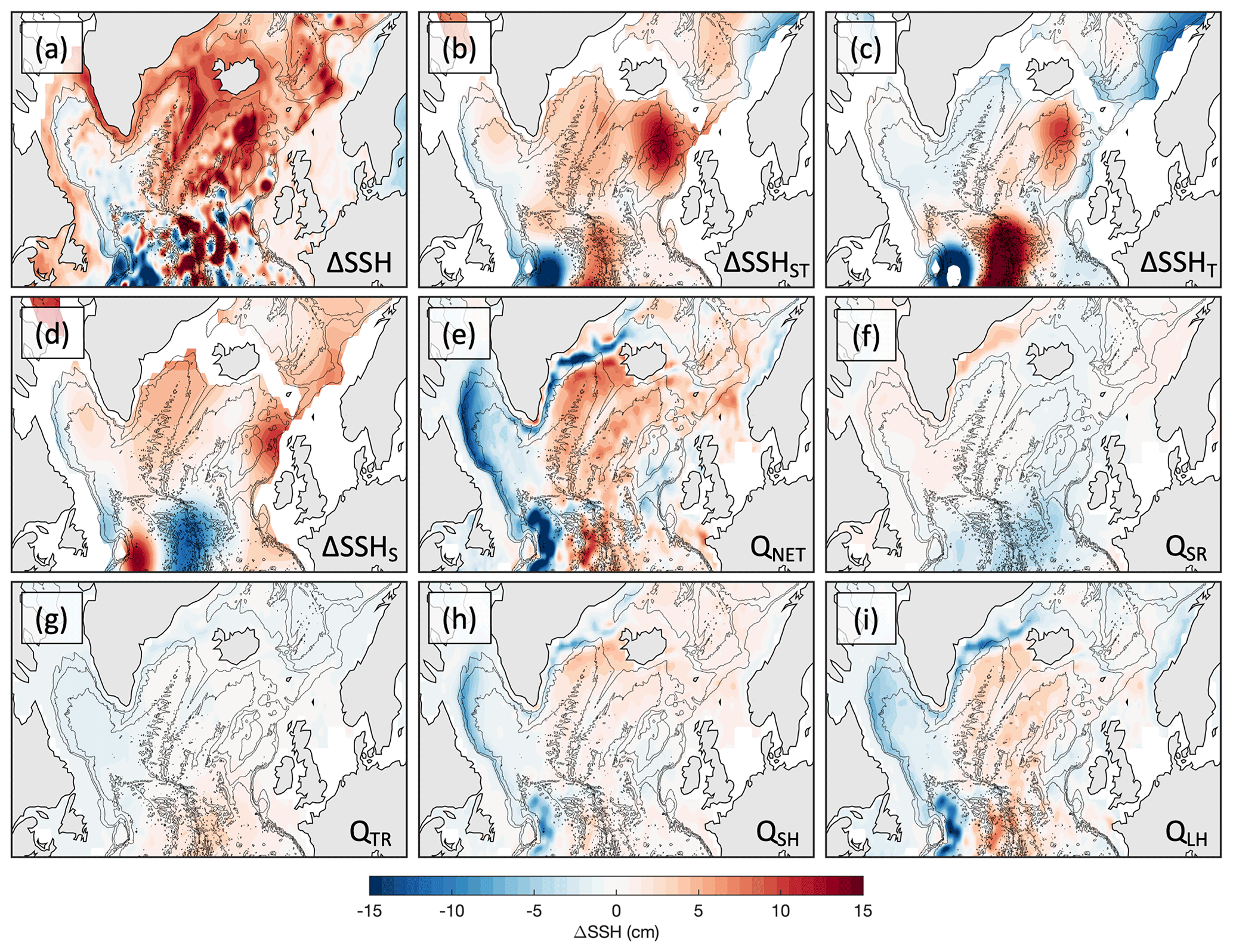
Figure 15 Same as Fig. 12 but for the 2015–2019 period.

During the following 2015–2019 period, SSH was rising in the northern and northeastern parts of the SPNA, particularly along the bottom topographic features associated with the Rockall Plateau and Reykjanes Ridge as well as along the Greenland shelf (Fig. 15a). Mostly, the observed SSH increase adequately compares to the SSH_ST increase (Fig. 15b). What is interesting to note is that this increase was not mainly determined by the SSH_T change as in the previous time intervals. The upper-ocean warming led to the SSH rise only in the Iceland Basin, over the Rockall Plateau, and further south upstream of the NAC (Fig. 15c). Warming in these areas was in part driven by the positive Q_NET anomalies (Fig. 15e) and by the advection of warmer and saltier water by the NAC (Fig. 15c, d). The positive Q_NET anomalies were also observed over the Reykjanes Ridge and in the Irminger Basin. However, these anomalies did not lead to upper-ocean warming and they were accompanied by a negative SSH_T tendency (compare Fig. 15e, c), which is suggestive of oceanic heat flux out of these areas. An anomalous heat loss to the atmosphere along the East Greenland Current (Fig. 15e), which was, however, associated with the local SSH increase, also suggests the dominant role of oceanic heat advection within the area influenced by the current. The largest contribution to the observed SSH rise in the interior of the Irminger Basin and Labrador Sea in 2015–2019 was provided by the upper-ocean freshening and the associated SSH_S rise (Fig. 15d). Because the impact of surface freshwater flux (P+E; not shown) is negligible, the observed freshening could only be driven by the advection of freshwater and/or the continental runoff, including the meltwater from Greenland glaciers. Similar to the previous time intervals, the contribution of the Q_SR and Q_TR anomalies to the Q_NET anomaly was small, and they balanced each other (Fig. 15f, g). The Q_NET anomaly was mainly driven by the Q_SH and Q_LH anomalies, with the largest contribution from the latter (Fig. 15h, i). Apparently, there was a tendency for the ocean to be colder than the atmosphere, thus favoring anomalous heat flux from the air into the ocean.

Figure 16 (a) Mean velocities at the 1000 dbar pressure level based on Argo float trajectories and Argo profiles of temperature and salinity; (b) eddy propagation velocities calculated from satellite altimetry data. The velocities were computed for the time period of 2005–2019.

4.6 The role of the large-scale ocean circulation in the SPNA

It is well known that persistent wind forcing leads to changes in the upper-ocean heat content through Ekman dynamics and the adjustment of the large-scale geostrophic circulation. In Sect. 4.4, we showed that the observed westward propagation of sea level anomalies in the SPNA is related to the shifts of NAO-like surface pressure and wind anomaly patterns. In the previous section, we demonstrated that while some of the observed regional tendencies of sea level can be explained by surface heat fluxes, there are regional tendencies that can only be accounted for by the advection of heat and freshwater. For example, the strong decrease in SSH–SSH_ST in 2011–2015 was mainly caused by the advection of colder and fresher water masses by the NAC (Fig. 14). In this section, we present the large-scale ocean circulation in the SPNA deduced from Argo trajectories at 1000 dbar depth (Fig. 16a) and from eddy propagation velocities calculated from satellite altimetry data (Fig. 16b), and we qualitatively analyze how ocean circulation could contribute to the observed westward propagation of SSH anomalies during the observational period.

The time-mean circulation at 1000 dbar depth shows a distinct cyclonic pattern constrained by bottom topography (Fig. 16a). This pattern is similar to the schematic upper-ocean circulation shown in Fig. 1 based on previous studies (e.g., Schmitz and McCartney, 1993; Schott and Brandt, 2007). The velocities derived from Argo trajectories correspond well to those derived from hydrographic sections and satellite altimetry (e.g., Sarafanov et al., 2012). The flow associated with the NAC, once it reaches the northern part of the Iceland Basin, recirculates southwestward along the eastern flank of the Reykjanes Ridge with speeds of about 5 cm s⁻¹. Upon crossing the Reykjanes Ridge, it follows its western flank, finally joining the system of western boundary currents composed of the East and West Greenland Currents and the Labrador Current, where the speeds often exceed 15 cm s⁻¹.

The eddy propagation pattern and speeds (Fig. 16b) are similar to the 1000 dbar velocities, meaning that eddies follow the mean SPNA circulation pathways, steered by bottom topography. Because the eddy propagation velocities (Fig. 16b) are directly derived from the SSH anomalies, they are representative of property transports in the upper ocean. Therefore, heat and freshwater signals advected to or generated in the Iceland Basin are transferred first to the Irminger Basin and then to the Labrador Sea. Assuming an average eddy propagation speed of 5 cm s⁻¹ (Fig. 16b), it takes about 1.5 years for an SSH signal to propagate from the northern part of the Iceland Basin (∼18^∘ W, 62^∘ N) to Cape Farewell and about 2 years to reach the northern part of the Labrador Sea at 63^∘ N following the mean circulation pathway along the eastern and western flanks of the Reykjanes Ridge and the Greenland continental shelf. This is the same timescale as the one we identified earlier using the CEOF analysis (see Sect. 4.3). Therefore, it is reasonable to suggest that the advection of heat and freshwater by the mean ocean circulation in the SPNA is a possible mechanism for the observed east-to-west propagation of SSH anomalies.

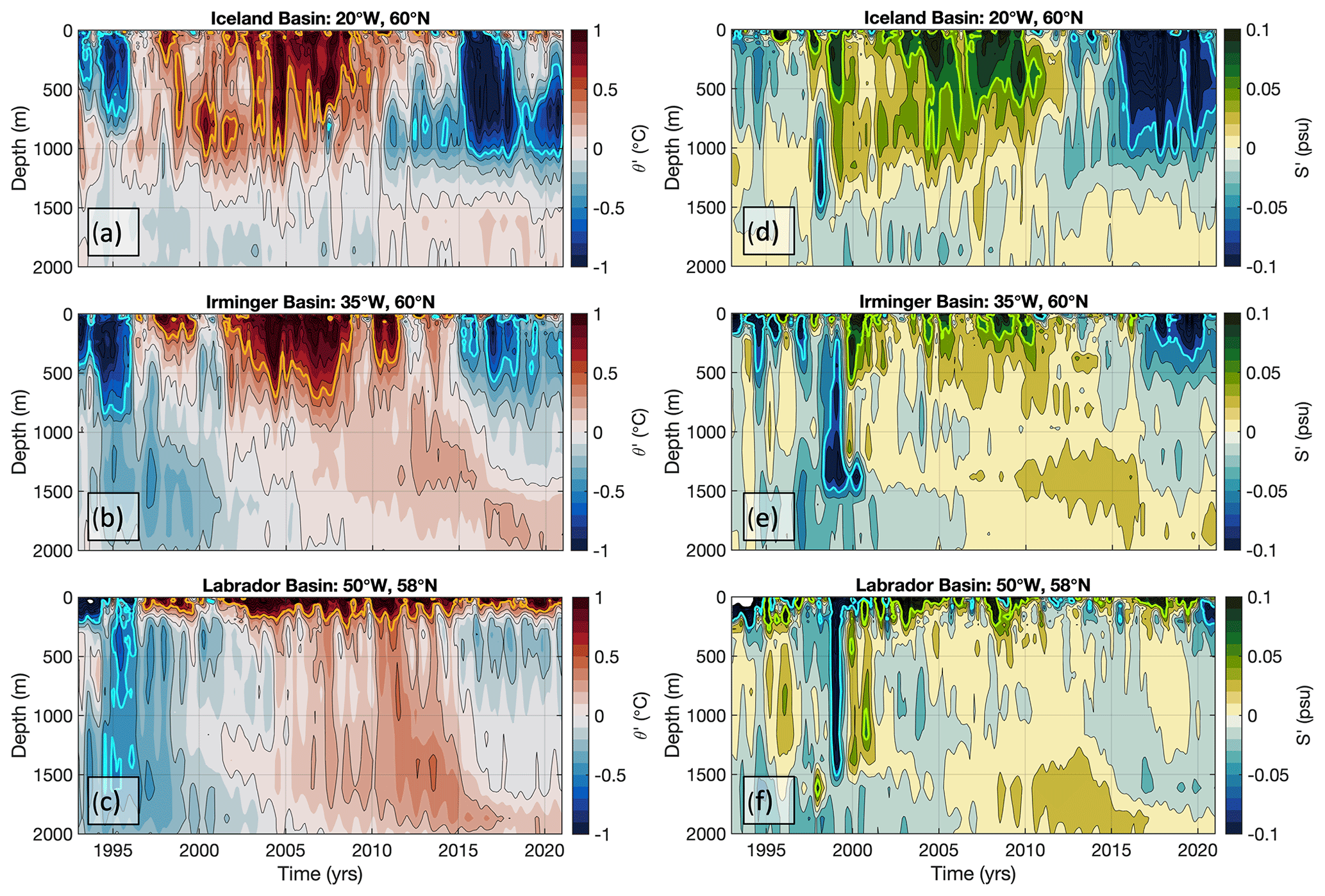
Figure 17 Anomalies of (a–c) potential temperature (with respect to the sea surface) and (d–f) salinity in (a, d) the Iceland Basin (at 20^∘ W, 60^∘ N), (b, e) the Irminger Basin (at 35^∘ W, 60^∘ N), and (c, f) the Labrador Basin (at 50^∘ W, 58^∘ N) (the locations are shown by red stars in Fig. 1). The orange and blue contours in (a–c) show 0.5 and −0.5 ^∘C isotherms, respectively. The green and blue contours in (d–f) show 0.06 and −0.06 psu.

To further illustrate the role of advection, we present time–depth diagrams of potential temperature and salinity anomalies from EN4 at three selected locations in the Iceland Basin (60^∘ N, 20^∘ W), in the Irminger Basin (60^∘ N, 35^∘ W), and in the Labrador Sea (58^∘ N, 50^∘ W) (Fig. 17). It should be noted that the EN4 data are more reliable after the Argo array achieved its complete coverage in the Atlantic in 2003. The anomalies that dominate the observed interannual to decadal SSH variability extend down to 1500–2000 m. Potential temperature anomalies (Fig. 17a–c) are driven by both the surface heat fluxes and the advection of heat. Because the impact of surface freshwater fluxes is very small (see Sect. 4.5), salinity anomalies (Fig. 17d–f) are mainly due to the advection of freshwater and continental runoff. The time–depth diagrams indicate that some anomalies are first observed in the Iceland Basin and then reach the Irminger Basin and the Labrador Sea. This is particularly evident in salinity anomalies, which are more representative of the impact of advection than temperature anomalies. For example, the negative potential temperature anomaly observed in the Iceland and Irminger basins in 1994–1995 reaches the Labrador Sea in 1–2 years. The 2015–2018 strong cooling anomaly in the Iceland Basin peaks in the Irminger Basin in 2017. The near-surface positive salinity anomaly observed in the Iceland Basin in 1998 reaches the Irminger Basin in 1999 and the Labrador Sea in 2000. The strong upper-ocean freshening observed in the Iceland Basin in 2015–2020 also reached the Irminger Basin 1–2 years later, and it only started to show up as subsurface freshening in the Labrador Sea in 2020.

5 Discussion and conclusions

This study presents a reconsideration of the interannual to decadal SSH variability in the North Atlantic, the leading mode of which exhibits a tripole pattern (Volkov et al., 2019b). The tripole was originally detected by the conventional EOF analysis (Fig. 2a, c; blue curve in Fig. 3), which is effective at depicting only standing oscillations. The sign of the tripole is mainly determined by SSH_T (Fig. 4a), partly balanced by a sizable contribution from SSH_S (Fig. 4d). The analysis presented here demonstrates that the first EOF mode alone does not adequately represent the interannual to decadal sea level variability in the SPNA. We show that the first mode explains the majority (60 %–90 %) of the interannual SSH variance only in the Irminger Basin and in the Labrador Sea (Fig. 5a), while the second EOF mode accounts for 60 %–80 % of the interannual SSH variance in the northeastern SPNA (Fig. 5b).

Furthermore, we demonstrate that the two modes do not represent two distinct physical processes. Instead, they belong to the same process and arise due to the general east-to-west propagation of SSH anomalies (Fig. 8). The CEOF analysis, which is designed to detect propagating (as opposed to standing) signals, yields the real and imaginary parts of the leading CEOF mode that correspond well to the first and second EOF modes, respectively. This suggests that the two leading EOF modes evolve as a quadrature pair associated with a propagation of SSH anomalies. Based on the CEOF analysis, there were almost three full cycles of the tripole-related SSH changes that exhibited westward propagation of SSH anomalies in the SPNA in 1993–2020 (Fig. 9). The reconstruction of the leading CEOF mode at different phases of one full cycle shows that SSH anomalies first appear along the northwestern European shelf and then gradually propagate westward (Fig. 8). It takes about 2 years for a signal to travel from the Iceland Basin to the Labrador Sea, and it takes 7–10 years for one full cycle to complete.

Because of the signal propagation, the concept of the North Atlantic SSH tripole introduced in Volkov et al. (2019) needs to be reconsidered, at least with respect to its application in the SPNA. While the standing oscillation of the interannual to decadal SSH anomalies is a reasonable approximation of the variability in the subtropical and tropical North Atlantic, signal propagation needs to be accounted for in the SPNA. Therefore, the tripole in the SPNA needs to be either based on the leading CEOF mode or on the first two EOF modes combined. It is necessary to mention that in order to describe the variability of SSH and ocean circulation in the SPNA, several authors have also used the subpolar gyre index, which, like the tripole, is based on an EOF decomposition of SSH fields (Häkkinen and Rhines, 2004; Hátún et al., 2005; Berx and Payne, 2017; Foukal and Lozier, 2017). The main difference between the subpolar gyre index and the tripole is that the global mean sea level is not subtracted from SSH fields prior to the computation of the former. Therefore, the subpolar gyre index exhibits a trend characteristic of the global mean sea level rise. The regional dynamic changes are then represented by higher modes, which led Hátún and Chafik (2018) to justly conclude that PC₂ in their calculation is a better metric for a gyre index than PC₁. Our results imply that with the signal propagation, if the global mean sea level is not subtracted prior to the EOF analysis, even the third mode needs to be considered.

To expand on the earlier work, we analyzed what mechanisms were responsible for the observed interannual to decadal SSH changes in the SPNA in 1993–2020 and what mechanisms could be responsible for the observed signal propagation. It has been documented that the North Atlantic SSH tripole is correlated with the NAO: stronger (weaker) than average midlatitude westerly winds associated with positive (negative) NAO phases lead to divergence (convergence) and lower (higher) sea levels in the SPNA (Volkov et al., 2019). We find that since the two leading EOF modes of the low-pass-filtered dynamic SSH depict the same physical process, the evolution of the second EOF mode is also related to an NAO-like dipole SLP pattern, but with shifted atmospheric pressure centers (Fig. 10). The definition of the NAO implies that it is a stationary standing oscillation pattern. However, the subtropical high-pressure and the subpolar low-pressure centers in the North Atlantic change both their intensity and position (e.g., Hameed and Piontkovski, 2004; Hameed et al., 2021). Therefore, we conclude that both the first and the second EOF modes may reflect oceanic response to the NAO-like persistent atmospheric forcing at different phases of its evolution. This conclusion is supported by the space and time evolution of SLP and wind anomaly patterns associated with the first CEOF mode of the low-frequency dynamic SSH (Fig. 11). The observed propagation of SSH anomalies from the eastern boundary towards the Labrador Sea corresponds to the westward shifts in atmospheric pressure and wind anomaly patterns (Figs. 8 and 11).

The role of surface buoyancy forcing over the SPNA in driving the interannual to decadal changes in SSH, SSH_T, and SSH_S is investigated over several characteristic time intervals: 1994–2010, 2004–2014, 2011–2015, and 2015–2019 (Figs. 12–15). The impact of surface freshwater fluxes is found to be negligible in all periods so that any changes in SSH_S are mainly driven by the advection of freshwater. Advection was apparently the main driver for the strong upper-ocean freshening observed in the eastern SPNA after 2010 (Figs. 7a, 14d). We find that the net surface heat flux anomalies, mainly caused by the sensible and latent heat flux anomalies, can fully or partly explain some regional tendencies in SSH_T. For example, Q_NET anomalies drove the increase in SSH_T in the Labrador Sea in 1994–2010 (Fig. 12c, e) and in the Iceland Basin in 2015–2019 (Fig. 15c, e), as well as the decrease in SSH_T in the northeastern SPNA in 2004–2014 (Fig. 14c, e) and in the Labrador Sea in 2011–2015 (Fig. 15c, e). However, there are regions and time periods in which changes in SSH_T can only be explained by advection, the contribution of which cannot not be directly estimated from observations. These are the regions and periods in which changes in SSH_T are either much larger or have a sign opposite to the changes implied by the Q_NET anomalies. A prominent example is a strong cooling in the SPNA in 2011–2015, known as the cold blob, which coincided with contemporary freshening (Fig. 14c, d). This period was apparently characterized by the advection of colder and fresher water masses into the region, consistent with findings of Holliday et al. (2020).

In addition to shifting atmospheric pressure patterns, the observed westward propagation of SSH anomalies could be caused by the mean ocean circulation in the SPNA. It appears that while the overall propagation is westward, SSH anomalies associated with EOF₁ and EOF₂ first spread over the shallower areas in the east-northeast, including the currents along the eastern and western flanks of the Reykjanes Ridge and the East Greenland Current (EOF₂; Figs. 2b and 5b), and then they reach the deeper parts of the Irminger Basin and Labrador Sea (EOF₁; Figs. 2a and 5a). The horizontal transfer of signals from the currents to the interior basins may be carried out by eddies generated by the boundary currents (e.g., Fan et al., 2013; de Jong et al., 2014). The likely role of ocean currents is qualitatively assessed using the climatological velocities at 1000 dbar obtained from Argo trajectories (Fig. 16a) and eddy propagation velocities estimated from satellite altimetry measurements (Fig. 16b). Both velocities depict the cyclonic circulation in the SPNA, constrained by bottom topography. The eddy propagation velocities signify the propagation of SSH anomalies, and therefore they are characteristic for the depth-integrated temperature and salinity (that define density and consequently SSH) transports. We find that the time required for SSH anomalies to propagate from the Iceland Basin to the Labrador Sea (1–2 years) is consistent with the time implied by the velocity estimates and by the upper 2000 m temperature and salinity anomalies (Fig. 17). This means the observed westward propagation of SSH anomalies is partly due to the mean direction of ocean currents in the SPNA. Any anomaly generated locally by atmospheric forcing or advected from another region is ultimately carried towards the Labrador Sea by ocean currents.

It should be noted that, due to geostrophy, both the SSH and the general ocean circulation are linked, and both adjust to persistent atmospheric forcing. For example, an increase in SSH along the European coast starts when the negative (cyclonic) SLP anomaly is centered over the eastern coast of Greenland and winds near the northwestern Europe are downwelling-favorable (phase 0^∘ in Figs. 8 and 11). As the cyclonic SLP anomaly weakens and moves towards the Labrador Sea (phase 45^∘ in Fig. 11), the subpolar gyre weakens and contracts, and the positive SSH anomalies near the eastern boundary expand westward (phase 45^∘ in Fig. 8). It has been reported that such situations can facilitate inter-gyre exchange: in response to a weakening of the subtropical high-pressure and subpolar low-pressure centers, the subtropical and the subpolar gyres weaken, sea level decreases in the subtropical gyre and increases in the subpolar gyre, the subpolar front moves westward, and the eastern boundary region in the SPNA widens, entraining more warm and saline waters from the subtropical gyre (Häkkinen et al., 2011; Piecuch et al., 2017). Consequently, positive SSH anomalies emerge first near the eastern boundary of the SPNA and then expand westward as the subpolar gyre continues to weaken (phases 45 to 180^∘ in Fig. 8). The opposite occurs when the subtropical and subpolar gyres strengthen (phases −135 to 0^∘ in Fig. 8). As demonstrated by the CPC₁ (Fig. 9), the local maximum SSH anomalies occurred in the eastern SPNA around 1996, 2004, and 2009, and they reached the western SPNA 1–2 years later. The most recent increase in SSH in the eastern SPNA since 2014 and in the western SPNA since 2016, that remains present in 2020, represents a recovery from an exceptional cooling and freshening that occurred in the SPNA in 2012–2016. This suggests that the recent conditions might again be favorable for inter-gyre exchange.

Overall, we conclude that the observed interannual to decadal variability of SSH, including the westward propagation of SSH anomalies, is the result of a complex interplay between the local surface wind and buoyancy forcing, as well as the advection of properties by mean ocean currents. The relative contribution of each forcing term to the variability is space- and time-dependent and therefore difficult to assess with available observations. The observed east-to-west propagation of SSH anomalies in the SPNA suggests the potential predictability of SSH changes and conditions favoring deep convection events in the region. This study puts the interannual to decadal changes in SSH in the SPNA in a broader context of the gyre-scale SSH variability in the entire North Atlantic. A caveat of this study is that it is based on a rather short observational record, which covers only a few cycles of the tripole-related variability. More observations are required to explore the persistence of the SSH signal propagation in the SPNA and to assess the characteristic timescales. In the meantime, it is possible to use longer SST records in a follow-on study. While we identify shifting wind forcing patterns and the mean ocean circulation as possible drivers for the observed westward propagation of SSH anomalies in the SPNA on interannual to decadal timescales, which process is more important remains unexplored. Further research is needed to understand the mechanisms of air–sea coupling in the SPNA, including potential oceanic feedback on the atmospheric circulation. Finally, it is of particular interest to explore how the tripole variability is related to inter-gyre exchange and to the AMOC.