Modelling the impact of anthropogenic measures on saltwater intrusion in the Weser estuary

The Weser estuary has been subject to profound changes in topography in the past 100 years through natural variations and river engineering measures, leading to strong changes in hydrodynamics. These changes are also expected to have affected the dynamics of saltwater intrusion. Using numerical modelling, we examined saltwater intrusion in the Weser estuary in four different system states (1966, 1972, 1981, 2012). Models of each system state were set up with the respective topography and boundary values. We calibrated and validated each model individually to account for differences in sediments, bedforms, and the resolution of underlying bathymetric data between historical and recent system states. In simulations of 1 hydrological year, each with realistic forcing (hindcasting study), the influence of topography is overshadowed by the effects of other factors, particularly river discharge. At times of identical discharge, results indicate a landward shift of the salinity front between 1966 and 2012. Subsequent simulations with different topographies but identical boundary conditions (scenario study) confirm that topography changes in the Weser estuary affected saltwater intrusion. Solely through the topography changes, at a discharge of 300 m³ s⁻¹, the position of the tidally averaged and depth-averaged salinity front shifted landwards by about 2.5 km between 1972 and 1981 and by another 1 km between 1981 and 2012. These changes are significant but comparatively small, since due to seasonal variations in run-off, the tidally averaged saltwater intrusion can vary by more than 20 km. An analysis of the salt flux through a characteristic cross section showed that saltwater intrusion in the Weser estuary is primarily driven by tidal pumping and only to a lesser degree due to estuarine circulation. However, results indicate that the contribution of individual processes has changed in response to anthropogenic measures.

1 Introduction

Estuaries are ever-changing systems. Natural processes and anthropogenic interventions determine the topography and conditions we observe in estuaries today. Due to the high economic importance of estuaries as shipping routes, further interventions to consolidate navigation channels can be expected. In order to manage adverse effects, predictability of changes associated with the engineering measures is essential. As a response to deepening measures, significant changes in hydrodynamics have been observed in estuaries. When water depth increases, the effect of bottom friction decreases. This reduces the dissipation of tidal energy, resulting in a larger tidal amplitude and often in phase shifts in the ebb and flood current durations and velocities (Winterwerp et al., 2013; Ralston et al., 2019). At the same time, changes in mixing processes can occur, possibly affecting the length of saltwater intrusion (Grasso and Le Hir, 2019). Saltwater intrusion is directly linked to water quality and sediment transport processes (Burchard et al., 2018) and thus needs to be monitored.

The effect of topography changes on saltwater intrusion depends on the physical mechanisms that control salt transport in estuaries. Most important are the net advection, driven by freshwater discharge, tidal asymmetry effects, and the estuarine circulation, i.e. the tidally averaged estuarine exchange flow. One driver of the estuarine circulation is the combination of the seaward barotropic (depth-independent) and the landward baroclinic (increasing with depth) pressure gradient, which results in a seaward flow of estuarine water near the surface and landward flow of dense water near the bed. This is known as the gravitational circulation (Geyer and MacCready, 2014). Depending on the estuary's geometry and tidal forcing, strain-induced periodic stratification (SIPS) can occur with stratification during ebb and mixing during flood (Simpson et al., 1990). This tidal asymmetry enhances estuarine circulation (Jay and Musiak, 1994) and has been referred to as “tidal straining circulation” (Burchard et al., 2011; Geyer and MacCready, 2014) or “eddy viscosity–shear covariance” (ESCO, Dijkstra et al., 2017). Salt transport is also controlled by, e.g. lateral momentum advection (Burchard et al., 2011) and estuarine convergence (Ianniello, 1979; Burchard et al., 2014). The strength of salt transport mechanisms depends on the water depth and it is therefore expected that channel deepening affects saltwater intrusion (Andrews et al., 2017).

Studies have been conducted in estuaries worldwide to try to quantify the impact of changes in topography, i.e. channel deepening or widening, on saltwater intrusion. In recent studies, numerical models with different topographies have been used to examine mixing and transport processes in estuaries before and after the implementation of engineering measures. Among others, such investigations have been conducted for the San Francisco estuary, US (Andrews et al., 2017), the Hudson River estuary, US (Ralston and Geyer, 2019), the Danshui River estuary system, Taiwan (Liu et al., 2020), the Seine estuary, France (Grasso and Le Hir, 2019), and the Ems estuary, Germany (van Maren et al., 2015).

Generally, it was found that a deepening of the river channel is associated with a landward shift of the brackish water zone. Several studies explain the increase in landward salt transport with an increase in the estuarine circulation and a decrease in vertical mixing processes, which occur due to the larger water depths (Grasso and Le Hir, 2019; Andrews et al., 2017; van Maren et al., 2015). In the case of the Danshui river estuary, some channels have been deeper in the pre-development state, which is accompanied by increased gravitational circulation and a further landward limit of the saltwater intrusion in the pre-development state (Liu et al., 2020). All the other aforementioned estuaries are deeper in the present state. Grasso and Le Hir (2019) investigated key estuarine processes in the Seine estuary in 1960 and 2010 and detected a relative increase in gravitational circulation and stratification. This caused an up-estuary shift of the salinity front and changed the response of saltwater intrusion to tides and discharge. Ralston and Geyer (2019) examined the Hudson River estuary in the present state and the pre-development state. They detected an increase in saltwater intrusion and stratification, but only a minor change in estuarine circulation and no change in the response of saltwater intrusion to river discharge. The authors concluded that dredging in the Hudson did not significantly change estuarine exchange processes.

In most of the aforementioned studies, a numerical model of the respective estuary in the present state was set up and calibrated. Different model topographies were subsequently inserted to represent earlier states of the estuary (Ralston and Geyer, 2019; Grasso and Le Hir, 2019; Liu et al., 2020). Models representing earlier system states of the estuary were not calibrated. However, differences in bed roughness are expected to occur between the system states due to sediment redistribution and changes in bed forms, which are usually not resolved in the models. Van Maren et al. (2015) calibrated models of the Ems estuary for different system states and obtained significantly larger roughness values with historical bathymetries compared to the present state. This is attributed to the observation that sediment in the Ems estuary has successively become finer in the past decades. The authors concluded that changes in bed roughness can strongly contribute to shifts in hydrodynamics and transport processes. In addition to shifts in bed roughness, the resolution of data which are used to generate model topographies may differ for the system states, which can have an effect on form drag. When setting up models with different topographies, individual calibration of each model might thus be advantageous.

In the Weser estuary, no model-based examinations have yet been conducted to examine the effect of anthropogenic measures on saltwater intrusion. Instead, saltwater intrusion and influencing parameters have been tracked by measurements and it was attempted to separate the impact of different factors (Krause, 1979; Grabemann et al., 1983). However, many factors affect saltwater intrusion on different time scales and it has thus not been possible to isolate the impact of topography variations (Grabemann et al., 1983). Within each tidal cycle, the position of the brackish water zone shifts by more than 15 km along the navigation channel of the Weser (Kösters et al., 2014). Changes in tidal components, meteorological conditions, long-term variations of the salinity of the North Sea, and variations in discharge also affect the position of the brackish water zone (Grabemann et al., 1983). Due to variations in discharge, the tidally averaged saltwater intrusion shifts by more than 20 km, whereby the impact of discharge variations is larger for low-discharge than for high-discharge conditions (Kösters et al., 2014).

This study aims to systematically quantify saltwater intrusion in a real tidal estuary in different system states and to determine to what degree anthropogenic measures, in particular deepening measures, impact saltwater intrusion in the estuary. As an example, we studied the Weser estuary in the German Bight and set up numerical model simulations in four different system states (1966, 1972, 1981, 2012). In contrast to most previous studies, we individually calibrated each model and conducted simulations with realistic and with idealized forcing. In this paper, we describe the model set-up and simulation results. We discuss the methodology, the importance of calibration for the model-based examination with different model topographies, and the effect of channel deepening on processes governing saltwater intrusion, i.e. the barotropic flux, tidal pumping, and the estuarine circulation for a characteristic cross section in the brackish water zone.

2 Study site: the Weser estuary

2.1 Geomorphology and hydrology

The Weser estuary, located in northern Germany, is of high ecological and economic importance. It is divided into two sections: the Lower Weser and the Outer Weser (see Fig. 1). The Lower Weser stretches from the tidal weir at Bremen-Hemelingen (km 0, the tidal limit) to Bremerhaven (km 66.7). The funnel-shaped Outer Weser starts from Bremerhaven and opens towards the North Sea (Weser-km 126). The estuary is an important shipping channel, providing access to the container terminal of Bremerhaven, the port of Bremen, and several smaller ports. During 1941–2015, the mean annual discharge, measured at the Intschede station, was 321 m³ s⁻¹ with high seasonal variability (NLWKN, 2018). In the same period, the mean annual minimum discharge was 116 m³ s⁻¹ and the mean annual maximum discharge was 1200 m³ s⁻¹ (NLWKN, 2018).

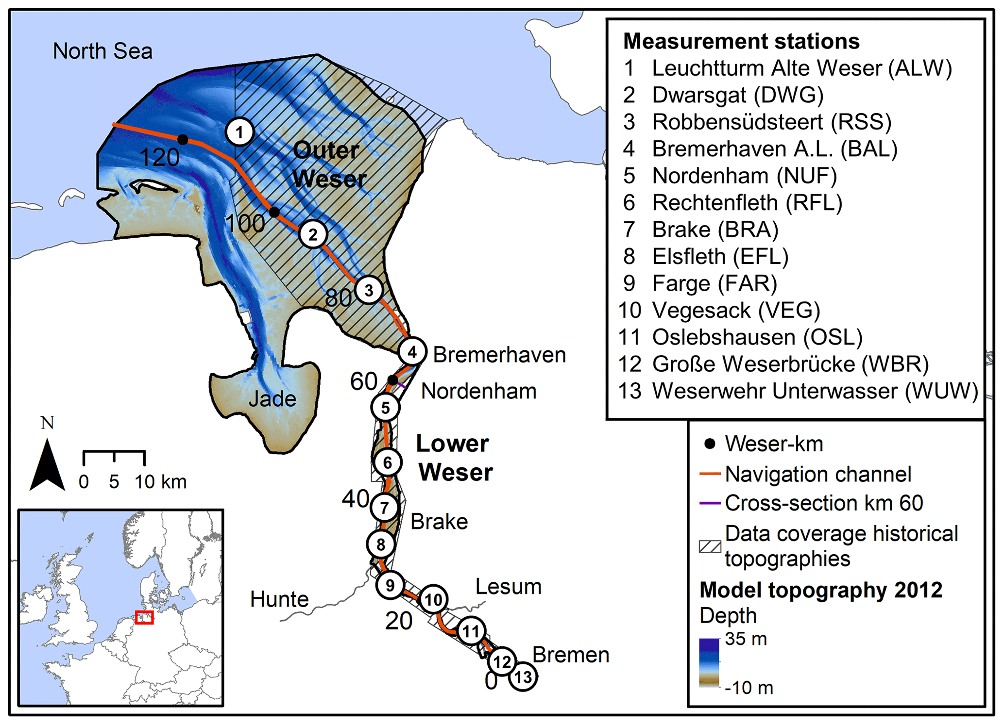
Figure 1 Map of the model area with the model topography 2012 displaying measurement stations and the distance along the navigation channel from the tidal weir at Bremen (Weser-km). The hatched area shows the data coverage for historical topographies.

The semidiurnal tidal wave from the North Sea propagates through the Weser estuary in about 3 h. At the northern part of the Outer Weser, the tidal range is 2.8 m. On its way through the estuary, it increases to 3.8 m near Bremerhaven due to estuarine convergence, slightly decreases between Weser-km 50 and 30, and increases to 4.1 m near Bremen. In most stretches of the navigation channel of the Lower and Outer Weser, ebb currents are slightly stronger than flood currents. Flood currents dominate in some stretches, such as Weser-km 80–95 (Lange et al., 2008).

Before mixing with seawater, the Weser River has an initial salinity of about 0.5 psu as a caustic potash solution is discharged further upstream. The mean position of the 2 psu isohaline is located at Weser-km 45 at the reversal from flood to ebb (high water slack) and Weser-km 60 at the reversal from ebb to flood (low water slack) (Lange et al., 2008).

2.2 Historical development

The topography of the Weser estuary has been significantly altered through river deepening and correction measures since the end of the 19th century. The main objective of these measures was to establish and maintain a continuous shipping route with sufficient depth and width for ships of increasing size to pass through (Lange et al., 2008).

Figure 2 Height along the navigation channel (200–300 m width) in the Weser estuary in different years, based on model topographies (a). Element height in a section of the Lower Weser of model topographies 1972 (b) and 2012 (c). Notations 48, 49, and 50 in (b) and (c) mark the position (Weser-km) along the navigation channel.

Since 1960, three major deepening measures have been conducted. The Outer Weser was modified during 1969–1971 to create a continuous depth of nautical chart datum “Seekartennull” (SKN) −12 m and during 1998–1999 to increase the depth to SKN −14 m (Lange et al., 2008). Engineering measures at the Lower Weser were conducted during 1973–1978. Thereby, the stretch between Brake (Weser-km 39) and Bremen (Weser-km 0) was deepened to nautical chart datum SKN −9 m, and the stretch between Bremerhaven and Nordenham to SKN −11 m (Lange et al., 2008). Starting in 1982, additional groynes were constructed in the Lower Weser to regulate the flow further. The mouth of the Ochtum tributary was relocated during 1972–1976, and the mouth of the Hunte tributary in 1979. Moreover, regular dredging measures for maintenance were conducted in the navigation channel (Lange et al., 2008). The bathymetry height along the navigation channel in the four system states is depicted in Fig. 2a.

3 Methods

We built numerical models of the Weser estuary in four system states: 1966, 1972, 1981, and 2012. A simulation of 1 hydrological year was conducted for each model with realistic forcing to hindcast hydrodynamics and saltwater intrusion (“hindcast study”). Results from previous calibration runs with respective topographies were used as initial conditions and a spin-up time of 4 weeks was applied. Additionally, simulations of each system state, but with identical forcing, were conducted and analysed for one spring–neap cycle (after a 6-week spin-up time) so that the impact of topography changes and roughness changes could be individually evaluated (“scenario study”).

3.1 Description of the numerical model

Numerical simulations are based on UnTRIM² (Casulli, 2008). UnTRIM² solves the Reynolds-averaged Navier–Stokes equations, the continuity equation, and transport equations based on a semi-implicit finite volume $/$ finite difference approach to calculate current velocities, surface elevations, and tracer concentrations (Casulli and Walters, 2000). The equations are solved on a horizontally unstructured grid with vertical z layers of 1 m thickness. The model considers 3D hydrodynamics, daily freshwater discharge from the Weser, and the transport of salinity and heat. Vertical turbulent mixing was estimated with a two-equation k-ε model; horizontal mixing was modelled with a constant viscosity (0.1 m² s⁻¹) and diffusivity (0.1 m² s⁻¹) in all simulations. UnTRIM² was coupled with the sediment transport model SediMorph (BAW, 2005), but only to calculate bottom roughness. Sediment transport was neglected in this study. The model is well-suited to simulate flows in estuaries, as the algorithm accurately preserves mass where wetting and drying occurs (Casulli, 2008). For example, it has been used to simulate flows in the San Francisco Bay (Andrews et al., 2017), the German Bight (Hagen et al., 2021b; Rasquin et al., 2020), and the Weser estuary (Kösters et al., 2014).

3.2 Model topographies

The model area includes the Lower Weser, the Outer Weser, and the adjacent Jade (see Fig. 1). Tributaries of the Weser and their discharge are not represented, because bathymetric and hydrographic data of the tributaries are not available for all system states. The same unstructured orthogonal calculation grid was used in all models. It contains cells of different sizes, arranged to increase the resolution in areas of interest. Cell spacing in the navigation channel is 50–250 m.

Model topographies were created by interpolating respective topographical data on the calculation grid, smoothing transitions, and correcting essential landscape features. The accuracy of the data sets differs depending on the quality and density of the original data. The model topography of 2012 is based on airborne laser scanning (ALS) for flat areas, multibeam echo-sounding for deep channels, and single-beam echo-sounding for shallow areas. Older bathymetries are mostly based on single-beam echo-sounding measurements. For most of the Outer Weser, topographical maps at a scale of 1 : 20 000 containing tracks with 70–200 m distance were used. For the Lower Weser, measurements along cross sections with 125 m longitudinal spacing were used. Topographical measurement data were not available for all regions for each time period. For example, historical data for the northern Outer Weser were only available from nautical charts of 1970 with lower data density. With temporal and spatial interpolation, considering deepening measures, all data were compiled to historical topographies of the Lower and Outer Weser (see Fig. 1, hatched area) in different historical system states (BAW, 2020, 2021). We interpolated the bathymetric data from 1966, 1972, and 1981 on the computational grid preserving the wet volume, which ensures that the water volume in the model agrees exactly with the average depths of the bathymetric data. We then filled the remaining area of the North Sea and Jade with bathymetric data from 2012. Subsequently, we corrected important landmarks and structures such as summer dikes, side channels, constructions, and the transition between Outer Weser (historical bathymetric data) and Jade (bathymetric data of 2012) in the case of the model topographies 1966, 1972, and 1981.

Due to the differences in temporal and spatial data coverage, the quality and level of detail of the model topographies differ. For example, bedforms such as dunes landwards of Weser-km 55 (Lange et al., 2008) are represented in the model topography of 2012 as variations in depths (see Fig. 2c). Historical recordings were less detailed, i.e. model topographies of 1966, 1972, and 1981 generally do not contain information on bedforms. Hence, the older topographies are smoother than 2012 (see Fig. 2b). We account for the different resolutions of the underlying bathymetric data and their effect on form drag by individually calibrating the models of each system state with the respective topographies (see Sect. 3.6).

3.3 Initial sediment distribution

We prescribed an identical initial sediment distribution in all models based on diverse sediment samples as described in Milbradt et al. (2015). The sediment distribution represents the system state 2012; data from previous years were additionally used at locations with insufficient data coverage. The distribution comprises eight fractions of sediments: very coarse sand, coarse sand, medium sand, fine sand, very fine sand, coarse silt, medium silt, and fine silt. We use the same initial sediment distribution in all models because historical data to suitably represent changes in sediment distribution over time were not available. In the models, the initial sediment distribution is used for roughness calculation based on sediment type and bedform prediction (see Sect. 3.6).

3.4 Model forcing

As boundary conditions, we prescribed time series for salinity, temperature, and water level at the seaward boundary to the North Sea. We also provided salinity, temperature, and discharge of the Weser at the landward boundary. The hindcast study aimed to represent the system states as realistically as possible. Measurement values were retrieved from the Waterways and Shipping Authorities of Bremerhaven, Bremen and Hannoversch Münden (WSV, 2022) and time series were constructed by linear interpolation between observations. Measured values were available for most parameters, but not for water level and salinity at the seaward model boundary in the North Sea in 1966, 1972, and 1981 and for salinity and temperature at the landward boundary in 1966. For the water level, however, historical records for tidal high and low water levels were available for the station “Leuchtturm Alte Weser” (ALW, see Fig. 1) close to the model boundary. Thus, we generated a synthetic time series of 1965–2012 by reconstructing the astronomical tide at station ALW, fitting the signal to measured high water and low water values and inducing a phase shift and amplitude amplification to account for the distance of the station to the model boundary. Salinities at four positions along the open boundary were approximated utilizing neural networks of two layers (55 and 11 neurons) with a Levenberg–Marquardt algorithm. For each position, 100 networks were trained with salinity values of 1996–2016, which were extracted from a validated model of the German Bight, the EasyGSH model (Hagen et al., 2021a). As reference data, the tidal range and tidal mean water level at station ALW, salinity records at the Helgoland station (Wiltshire et al., 2008), and the discharge of the Weser and Elbe were used. Subsequently, the correlation of network results and the extracted target salinity values were calculated and the best network for each position was selected. With the selected networks, salinity at each position was predicted for all system states (1965–2012). For evaluation of the performance of neural networks, a skill estimator was applied according to Murphy (1988), implemented in the form suggested by Ralston et al. (2010).

$$\begin{array}{}\text{(1)}& \mathrm{MSS}=\mathrm{1}-{\displaystyle \frac{{\sum }_{i=\mathrm{1}}^N(X_{\mathrm{sim}}-X_{\mathrm{obs}}{)}^{\mathrm{2}}}{{\sum }_{i=\mathrm{1}}^N(X_{\mathrm{obs}}-{\stackrel{\mathrm{‾}}{X}}_{\mathrm{obs}}{)}^{\mathrm{2}}}}\end{array}$$

The Murphy Skill Score (MSS) compares the squared error between approximated values X_sim and observed values X_obs with the squared error between observed values and mean of observed values at each time step. It evaluates the prediction of the neural networks in comparison with the mean observed values. If the MSS < 0, the mean observed value is better than the prediction of the neural network and vice versa. The MSS of the selected networks ranges between 0.34 (western model boundary) to 0.7 (eastern model boundary), indicating that prediction with the neural networks was effective. Boundary values for salinity and temperature at the landward boundary for the hindcast model 1966 were reconstructed. For salinity, a relationship between discharge and salinity was derived based on measured data from 1967 to 1968, where the amount of potash discharging can be assumed to be similar to 1966. Salinity values for the hydrological year 1966 were calculated based on measured discharge values with

$$\begin{array}{}\text{(2)}& \begin{array}{rl}{S}_{\mathrm{river}}& =\mathrm{6}\cdot {\mathrm{10}}^{-\mathrm{7}}\mathrm{psu}{\mathrm{m}}^{-\mathrm{6}}{\mathrm{s}}^{\mathrm{2}}\cdot Q^{\mathrm{2}}\\ & -\mathrm{0.0017}\mathrm{psu}{\mathrm{m}}^{-\mathrm{3}}\mathrm{s}\cdot Q+\mathrm{2.0759}\mathrm{psu},\end{array}\end{array}$$

where S_river is salinity and Q is discharge. For temperature, measured values of 1968 were used instead of 1966, as the variations over the years were assumed to be similar and temperature is only of secondary importance in this study.

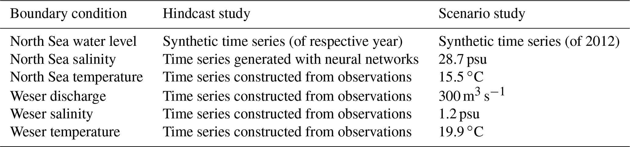
In contrast to the hindcast study, we used identical boundary values in all simulations for the scenario study. The synthetic time series of the hindcast model 2012 was used for water level at the open boundary. For all other parameters, cross-scenario boundary values were generated, representing an average of the four system states (see Table 1).

Table 1 Boundary values in hindcast study (realistic forcing) and scenario study (identical forcing). In each study, simulations of system state 1966, 1972, 1981, and 2012 were conducted.

3.5 Analysis methods

Model results were analysed by calculating tidal characteristic values, which describe the tidal curve and facilitate characterization of the system's behaviour and comparison between simulations (Lang, 2003). Thus, for example the tidal range and the minimum, mean, and maximum salinity per tidal cycle were calculated in each scenario and compared.

In addition, the position of the brackish water zone was calculated for all model results by determining the position of the 5 psu and 20 psu isohaline along the navigation channel (see Fig. 1) based on the tidal mean of the vertically averaged salinity. The saltwater intrusion length was defined as the distance from the estuary mouth (Weser-km 126.2, see Fig. 1) to the 5 psu isohaline along the navigation channel. In order to identify processes driving the saltwater intrusion, the following analysis methods have been applied.

3.5.1 Regression analysis

The effect of discharge on the saltwater intrusion length was quantified by means of a regression analysis based on data from the hindcast simulations. Saltwater intrusion was calculated for each tidal cycle in the respective hydrological years and discharge conditions were assigned. Data points were then sorted into 50 m³ s⁻¹ bins of discharge between 150 and 400 and 100 m³ s⁻¹ bins between 400 and 1100 m³ s⁻¹ and averaged to reduce the effect of additional factors and outliers. If fewer than 10 entries were available for a category, these entries were excluded. Based on the resulting average intrusion length for the specified discharge categories, multiple nonlinear regression with interaction effects was performed with the Levenberg–Marquardt algorithm to obtain trends of the form

$$\begin{array}{}\text{(3)}& L^{\ast }=k{Q}^m,\end{array}$$

with saltwater intrusion length L^∗, factor k, discharge Q, and exponent m. The analysis was repeated without data aggregation to examine the method's validity.

3.5.2 Salt flux decomposition

We decomposed the total salt flux F_tot into three components: barotropic flux F_bf, estuarine exchange F_exf, and tidal pumping flux F_tp. The method is based on the decomposition analysis of sediment fluxes of Becherer et al. (2016). We apply their method to analyse salt flux through a cross section in the Lower Weser (Weser-km 60, see Fig. 1), located in the brackish water zone of the estuary. We conducted the salt flux decomposition for equidistant points along the cross section (distance of 25 m) and integrated the results over the whole width of the cross section. In a first step, we interpolated our data on a σ-layer grid with M=50 equidistant layers. Then we calculated the temporal average of salinity s and current velocity in the main flow direction u at σ layers with

$$\begin{array}{}\text{(4)}& \langle X_{\mathit{\sigma }}{\rangle }_t={\left[\underset{t=\mathrm{0}}{\overset{T}{\int }}{h}_{\mathit{\sigma }}\left(t\right)\mathrm{d}t\right]}^{-\mathrm{1}}\underset{t=\mathrm{0}}{\overset{T}{\int }}{X}_{\mathit{\sigma }}\left(t\right)h_{\mathit{\sigma }}\left(t\right)\mathrm{d}t,\end{array}$$

where X is the respective quantity, h is the height of the σ layer, and T is the analysis period. Temporal averages are represented by angle brackets. Becherer et al. (2016) use a moving average window to track effects of variable forcing on the flux components. Since the simulations are run with constant river discharge as forcing and only contain variations in water level from the North Sea (see Table 1, scenario study), we can simply average over the entire analysis period of the scenarios (one spring–neap cycle). We calculated deviations from the mean, indicated by curly brackets, with

$$\begin{array}{}\text{(5)}& {\left\{X_{\mathit{\sigma }}\right\}}_t\left(t\right)=X_{\mathit{\sigma }}\left(t\right)-\langle X_{\mathit{\sigma }}{\rangle }_t.\end{array}$$

Vertical averages were calculated according to

$$\begin{array}{}\text{(6)}& \langle X{\rangle }_{\mathit{\sigma }}={\displaystyle \frac{\mathrm{1}}{M}}\sum _{\mathit{\sigma }=\mathrm{1}}^M{X}_{\mathit{\sigma }}.\end{array}$$

From the temporal and vertical averages and deviations, we determined the salt flux components and integrated them over the width W of the cross section.

$$\begin{array}{}\text{(7)}& \begin{array}{rl}{F}_{\mathrm{tot}}& =\underset{w=\mathrm{0}}{\overset{W}{\int }}\langle D{\rangle }_t\langle \langle s_{\mathit{\sigma }}{u}_{\mathit{\sigma }}{\rangle }_t{\rangle }_{\mathit{\sigma }}\mathrm{d}w\\ & =\underset{F_{\mathrm{bf}}}{\underbrace{\underset{w=\mathrm{0}}{\overset{W}{\int }}\langle D{\rangle }_t\langle s_{\mathit{\sigma }}{\rangle }_{t,\mathit{\sigma }}\langle u_{\mathit{\sigma }}{\rangle }_{t,\mathit{\sigma }}\mathrm{d}w}}\\ & +\underset{F_{\mathrm{exf}}}{\underbrace{\underset{w=\mathrm{0}}{\overset{W}{\int }}\langle D{\rangle }_t\langle \mathit{\{}\langle s_{\mathit{\sigma }}{\rangle }_t{\mathit{\}}}_{\mathit{\sigma }}\mathit{\{}\langle u_{\mathit{\sigma }}{\rangle }_t{\mathit{\}}}_{\mathit{\sigma }}{\rangle }_{\mathit{\sigma }}\mathrm{d}w}}\\ & +\underset{F_{\mathrm{tpf}}}{\underbrace{\underset{w=\mathrm{0}}{\overset{W}{\int }}\langle D{\rangle }_t\langle \mathit{\left\{}{s}_{\mathit{\sigma }}{\mathit{\}}}_t\mathit{\right\{}{u}_{\mathit{\sigma }}{\mathit{\}}}_t{\rangle }_{t,\mathit{\sigma }}\mathrm{d}w}}\end{array}\end{array}$$

The barotropic flux F_bf contains residual barotropic flows due to river discharge, barotropic ebb–flood asymmetries, and wind stress. The vertical exchange flow F_exf indicates the estuarine circulation and the tidal pumping flux F_tp indicates upstream transport by the correlation of salinity and velocity fluctuations (Becherer et al., 2016).

3.6 Calibration and validation

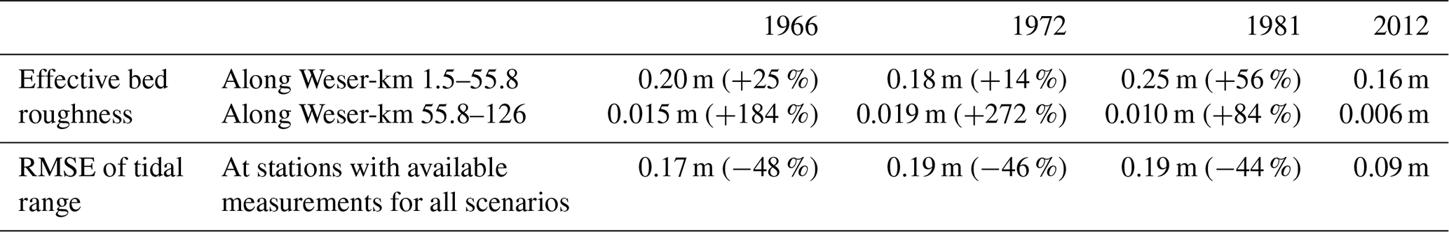
Models of each system state were calibrated in two steps by adjustment of the roughness settings: (1) tuning of a form roughness predictor, and (2) definition of an additional roughness in the Lower Weser. The simulation time for each system state was 4 weeks. Bottom roughness in our models is described by Nikuradse's effective roughness coefficient k_s, which relates to the bed roughness length z₀ with $z_{\mathrm{0}}\simeq k_{\mathrm{s}}/\mathrm{30}$ (Malcherek, 2010). In nature, roughness can be seen as the sum of grain- and form-related roughness. The sediment transport model SediMorph, which is coupled with the hydrodynamic model UnTRIM², calculates the grain roughness k_s,grain at each element from the prescribed sediment distribution with $k_{\mathrm{s},\mathrm{grain}}=\mathrm{3}{d}_{\mathrm{m}}$, where d_m is the mean grain size. Form roughness is estimated at each time step of the simulation based on sediment properties, water depth, and velocity, according to van Rijn (2007). Calibration factors, which determine the prevalence and importance of bedforms (ripples, mega ripples, dunes), were varied in the calibration to optimize the agreement between simulated and observed water levels, if available (system state 2012), high water and low water values (all scenarios), and the tidal range (all scenarios). The effect of dunes could not be reliably modelled with the predictor but had to be prescribed as an additional roughness landwards of Weser-km 55. The additional roughness also compensates model effects, such as due to the omission of the Weser's tributaries. Tributaries typically dampen the tidal wave through shallow water depths and high energy dissipation rates. The additional roughness increases from Weser-km 55 towards Weser-km 26 and decreases afterwards again. In this way, damping of the tidal wave could be well represented. Roughness as calculated by the numerical model (effective bed roughness) along the navigation channel is described in Table 2. For each model, different roughness settings were determined. While the estimated form roughness is in the range of 0.01–0.04 m, the maximum additional roughness ranges from 0.22 m (system state 2012) to 0.36 m (system state 1981). The mean RMSE of tidal range in scenarios 1966, 1972, and 1981 improved by almost 50 % after adjustment of the roughness settings by individual calibration (see Table 2).

Table 2 Effective bed roughness along the navigation channel of the Weser estuary (see Fig. 1) and RMSE of the tidal range for the individually calibrated models. For 1966, 1972, and 1981, results are compared with respective calculations with roughness settings of 2012 (before individual recalibration).

In other estuaries, changes in sediments and bedforms were observed over time. For example, dredging induced fine sediment accumulation in the Ems (Winterwerp et al., 2013; van Maren et al., 2015) and reduced drag associated with bedforms in Columbia River (Jay et al., 2011), both contributing to lower friction and an amplification of tides. There are no data to assess whether there have been comparable changes in sediment inventory in the Weser estuary. But the height of bedforms will almost certainly have changed with changing water depths. Such changes are not represented in our models, which could explain to some extent differences between scenarios.

In addition, effects induced by the different resolutions of the original bathymetric data (see Sect. 3.2) are balanced out through roughness calibration. To some extent, dunes are depicted in the numerical grids – if present in the bathymetric data. In the examined years prior to 2012, bathymetric data almost did not resolve dunes. This has an effect on depth variation in the model topographies and the associated form drag. The lesser depth variation in the older model topographies is compensated by defining a larger additional roughness. The largest additional roughness was required in the model of system state 1981 (see Table 2). The model topography includes the deepening of the Lower Weser to SKN −9 m in 1973–1978 (see Sect. 2.2), which led to strong changes in tidal dynamics. The model seems to overestimate this effect, possibly due to the limited model resolution and omission of tributaries. This could be outbalanced by the additional roughness. Possible tests to further evaluate the effect of the resolution of bathymetric data could include smoothing the 2012 model topography to be comparable to historical topographies and evaluating the effect on calibration results. Alternatively, the low resolution of historical bathymetric data could be compensated by adding artificial surface irregularities, which represent the depth variation due to, e.g. sand waves, as implemented by Hubert et al. (2021).

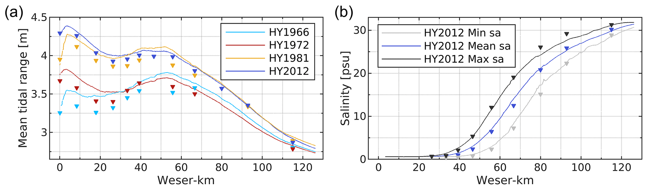
Figure 3 Mean tidal range along the navigation channel of the Weser estuary (see Fig. 1) in hindcast models of 2012, 1981, 1972, and 1966 (a) and vertically averaged mean, minimum, and maximum salinity per tide (average) in hindcast model HY2012 (b). Simulation results (lines) are compared with measured values (triangles), averaged over the same period.

The models were subsequently validated by extending the calculation time to 1 hydrological year (plus the preceding 4 weeks to allow for a model spin-up) and comparing model results with measurements. One hydrological year is the time between 1 November of the previous year and 31 October of the respective year (DIN 4049-1:1992-12, 1992). The tidal range in the Lower Weser was slightly overestimated in the hindcast models (see Fig. 3a), but overall well reproduced with a mean RMSE of 0.166 m (1966), 0.114 m (1972), 0.169 m (1981), and 0.153 m (2012), averaged over stations along the navigation channel with available measurements for all scenarios. Measured values of water level and salinity only covered system state 2012. The mean RMSE for the comparison of modelled and observed water levels in 2012 was 0.22 m, averaged over all measurement stations (see Fig. 1). An overall bias of 5 cm indicated a slight, consistent overestimation of water levels. A visual inspection of observed and modelled water levels suggested a correct phasing of tides, which is corroborated by the low RMSE. Saltwater intrusion was slightly overestimated, with higher computed values than measured values in Lower Weser (see Fig. 3b). The intratidal variation in Weser-km 60–100 was slightly underestimated, with higher minimum salinity and lower maximum salinity per tide. The mean RMSE in hindcast model 2012 was 1.4 psu for mean salinity, averaged over all stations with available measured values. Overall, the magnitude and dynamics of saltwater intrusion were reproduced well in the hindcast model 2012. It is expected that the model performance will be similar for the other system states.

4 Results

4.1 Natural variability of saltwater intrusion in the Weser estuary

To give an idea of the temporal variation of salinity in the Weser estuary, measurement data of the hydrological year 2012 are shown in Fig. 4. In each semi-diurnal tidal cycle, the 5 psu isohaline moves up- and downstream by almost 20 km (see Fig. 4a). It is located about 2–3 km further landwards during spring tide compared to neap tide. The mean position of the 5 psu isohaline per semi-diurnal tidal cycle shifts by more than 30 km in the year. A major seaward shift occurs in December and January, where the isohaline moves from Weser-km 40 to Weser-km 73. This is induced mainly by an increase in discharge from 100 to 1000 m³ s⁻¹.

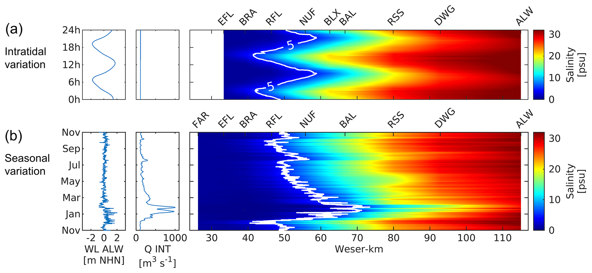
Figure 4 Intratidal and seasonal variation of saltwater intrusion in the Weser estuary. The water level at the Leuchtturm Alte Weser (ALW) station, discharge at the Intschede (INT) station, and salinity along the navigation channel of the Weser estuary are displayed on different time scales. Salinity values were interpolated linearly between measurement stations with available measurements along the navigation channel. The 5 psu isohaline is displayed in white. On top, salinity variation in 1 day, 1 September 2012, is depicted (a). Below, variation in the hydrological year 2012 of the mean salinity per tidal cycle is depicted (b). We applied a moving median filter to the water level data in (b) to show the seasonal variation (filter size 12 h 25 min).

4.2 Saltwater intrusion in different system states

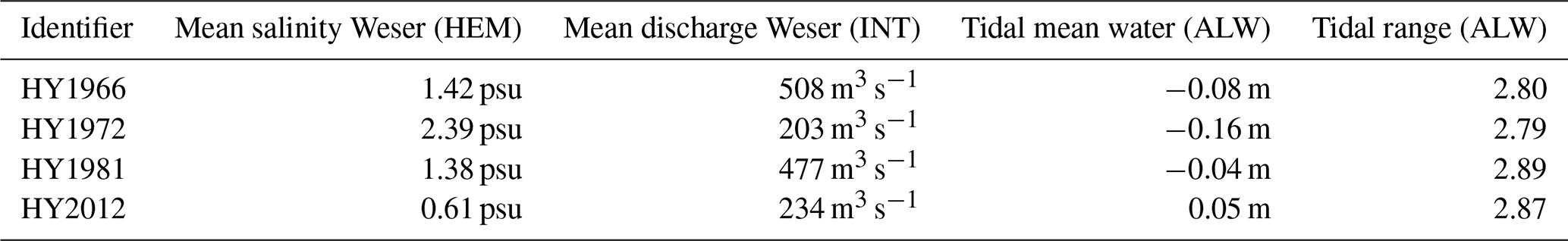
Hydrodynamics and saltwater intrusion in the Weser estuary were simulated in hindcast models of 1966, 1972, 1981, and 2012. These models contain respective model topographies and realistic forcing (see Table 1) and they were individually calibrated (see Sect. 3.6). The mean tidal range in the estuary is up to 0.6 m larger in 1981 and 2012 than in 1966 and 1972 (see Fig. 3a). This reflects the impact of the deepening measures in Lower Weser during 1973–1978, which had a strong effect on tidal dynamics. Saltwater intrudes further in 1972 and 2012 compared to 1966 and 1981 (see Fig. 5). In 1972 and 2012, the 5 psu isohaline is positioned about 10 km more landwards. The reason for these large differences is particularly high discharge values in 1966 and 1981, which were on average about twice as high compared to the other system states (see Table 3). Not all variation can be explained with the discharge conditions. Compared to 1972, there was higher discharge in 2012; however, the position of the salinity front is about 3 km more landwards. In this case, other influencing factors outweigh the impact of discharge. The mean tidal level at station ALW in system state 2012 was considerably higher compared to 1972, indicating different meteorological conditions and reflecting an increase in mean sea level (Wahl et al., 2013). Moreover, the tidal range at station ALW was larger in 1981 and 2012, possibly due to topography changes (Hubert et al., 2021) and in response to the nodal tide. Along with these factors, changes in topography might affect the differences in the saltwater intrusion.

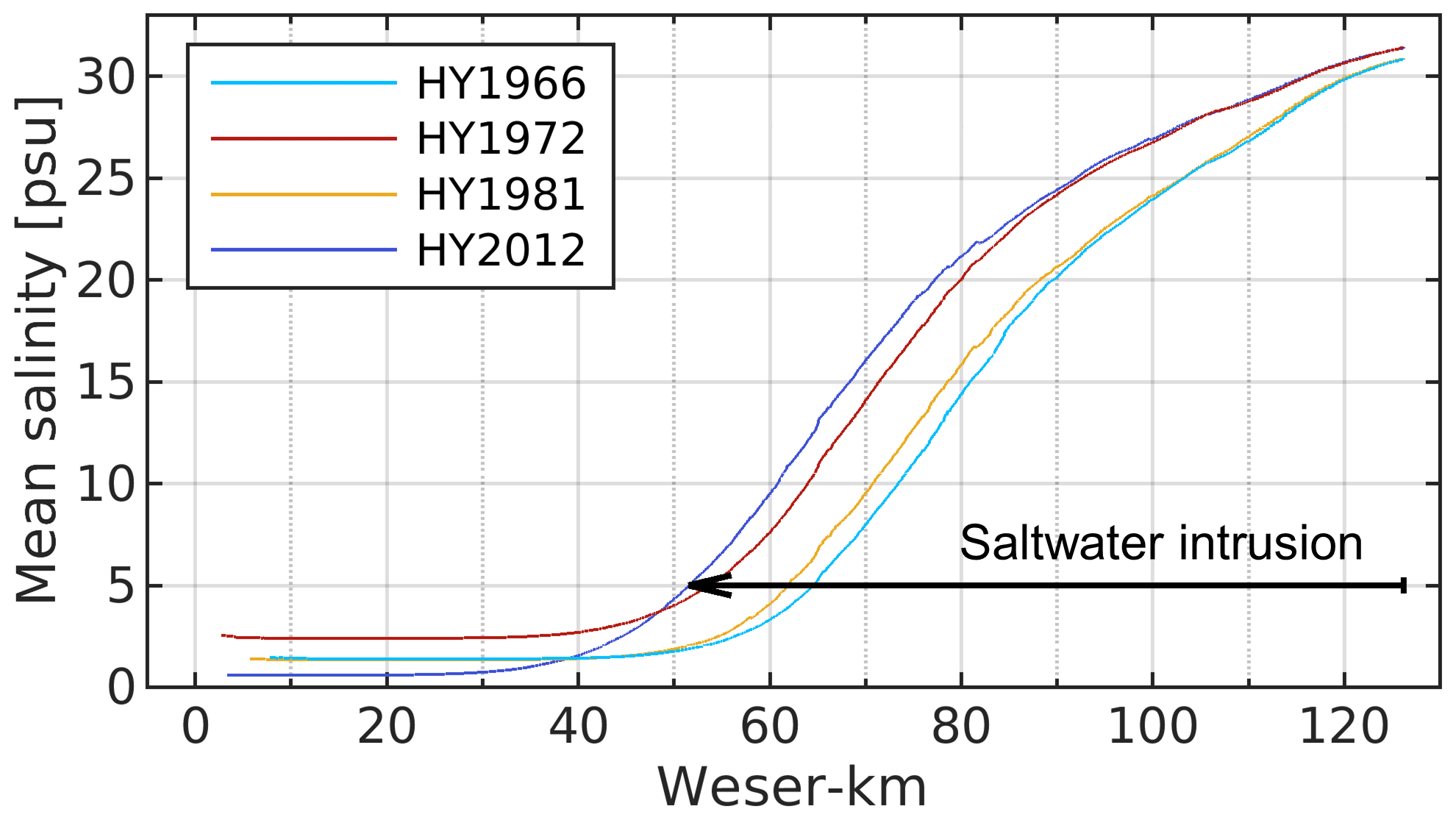
Figure 5 Annual mean, vertically averaged salinity along the navigation channel of the Weser estuary (see Fig. 1) in hindcast models of 1966, 1972, 1981, and 2012.

Table 3 Characteristic conditions in system states 1966, 1972, 1981, and 2012, averaged for 1 hydrological year based on measured values. Mean salinity and mean discharge were measured at Hemelingen (HEM) and Intschede (INT). Both stations are located upstream of the Bremen weir. Tidal mean water and tidal range in the North Sea were measured at Leuchtturm Alte Weser (ALW).

4.3 Effect of discharge on saltwater intrusion in different system states

The sensitivity of saltwater intrusion to discharge can be described with analytical expressions, which depend on dominant salt flux mechanisms and estuary shape. With a regression analysis (see Sect. 3.5.1), we examined the influence of discharge on the saltwater intrusion length in all hindcast simulations. Amongst the simulations, discharge and other parameters differ (realistic forcing, see Table 1). Two versions of the analysis were conducted: with and without pre-processing by data aggregation. Data from the hindcast simulation of 1972 were excluded because the range of discharge values was insufficient for the analysis.

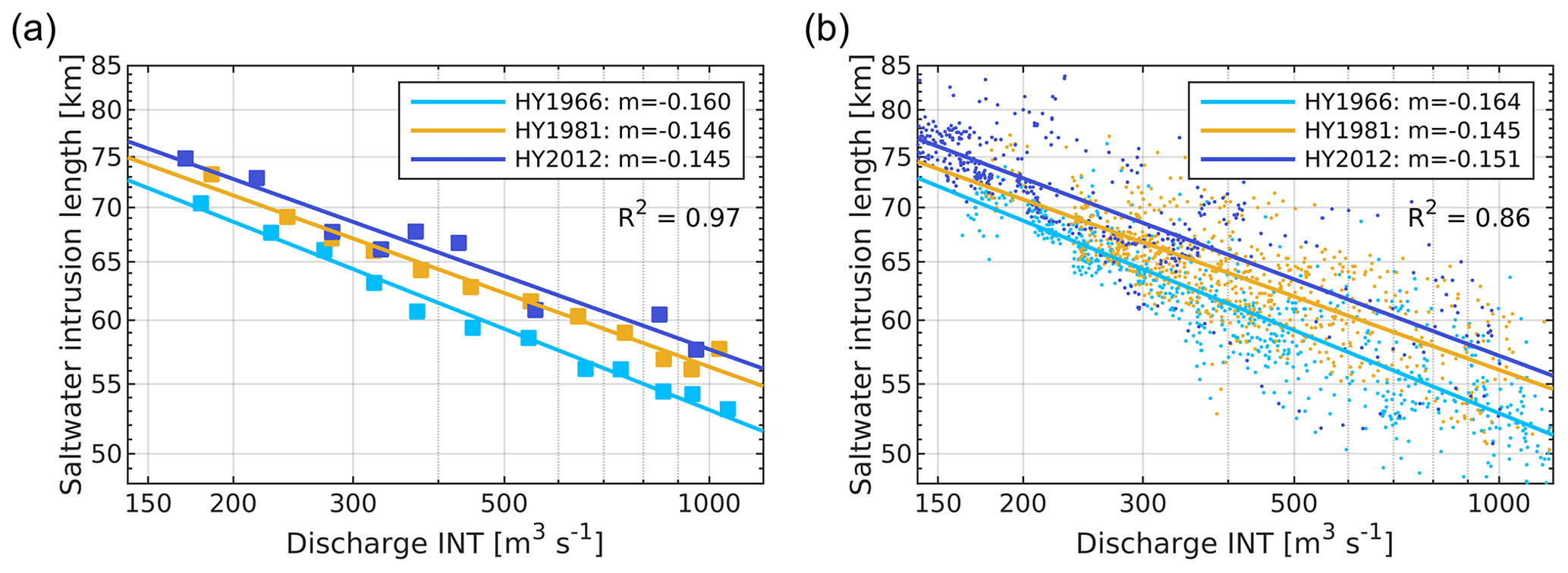
Figure 6 Saltwater intrusion length L^∗ (distance from the estuary mouth at Weser-km 126.2, see Fig. 1, along the navigation channel to the tide-averaged 5 psu isohaline) in hindcast models of 1966, 1981, and 2012, in relation to discharge Q measured upstream of Bremen weir at the Intschede (INT) station. On the left, squares represent the average saltwater intrusion length for different discharge categories and lines represent trends of the form $L^{*}=k{Q}^m$. With logarithmic scales, m represents the gradient of the lines (a). The analysis was repeated with non-aggregated data points to test the method's validity (b).

In the scenarios representing 1966, 1981, and 2012, we identified a clear relationship between discharge and saltwater intrusion length according to Eq. (3), with $L\sim Q^{-\mathrm{0.15}}$. In system state 2012, the saltwater intrusion length increases by approximately 9 km if the discharge decreases from 1000 to 380 m³ s⁻¹ or from 380 to 150 m³ s⁻¹. The trend lines for 1966, 1981, and 2012 have comparable gradients in the logarithmic plot (comparable exponents m, see Fig. 6). A significant difference occurs between the exponent in HY1966 compared to the exponent in HY1981 (p<0.001) and HY2012 (p=0.005) in the regression analysis with non-aggregated data points.

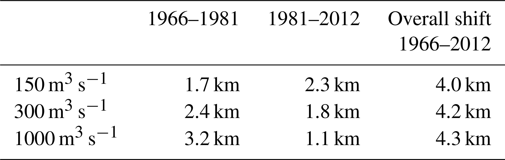
The shift in trend lines indicates that saltwater intrusion increased between 1966 and 1981 and between 1981 and 2012 for similar discharge conditions (see Table 4). For example, with 300 m³ s⁻¹ discharge, the saltwater intrusion increased by approximately 2.4 km between 1966 and 1981 and another 1.8 km between 1981 and 2012. This trend could be linked to differences in topography, i.e. the deepening measures conducted between the system states.

Table 4 The average landward shift of the 5 psu isohaline in the hindcast simulations, based on regression analysis (see Fig. 6b).

4.4 Impact of topography changes on saltwater intrusion

The effect of topography on saltwater intrusion was further examined in simulations with identical boundary values but different model topographies (scenario study). One set of simulations (1966, 1972, 1981, 2012) was conducted with the respective roughness settings, as obtained by calibration of the hindcast models. Another set of simulations was conducted with identical roughness settings (hindcast model 2012). Simulations with different topographies and respective roughness settings confirm a notable effect of topography changes on saltwater intrusion (see Fig. 7a). The salinity front (5 psu isohaline) shifts landwards between scenario 1972 and 1981 by about 2.5 km, and between 1981 and 2012 by another 1 km. At the same time, the length of the brackish water zone (5 psu isohaline to 20 psu isohaline) increases between the four scenarios from 24.2 km (1966) to 27.6 km (2012).

The differences in saltwater intrusion can be linked to the topography changes between the four system states. The most significant increase in saltwater intrusion occurs between scenarios 1972 and 1981, where considerable deepening measures were conducted in the Lower Weser. An analysis of the mean depth of the navigation channel in the area where saltwater intrusion occurs (Weser-km 40–110) and the position of the 5 PSU isohaline in each of the scenarios suggests a strong link between mean depth and saltwater intrusion (see Fig. 7b). According to this, if the navigation channel is deepened by 1 m in Weser-km 40–110, the position of the 5 psu isohaline shifts landwards by about 2 km. Deepening measures in the Outer Weser seem to induce an overall extension of the brackish water zone. Between scenario 1966 and 1972 and between scenario 1981 and 2012, when deepening measures in the Outer Weser were conducted, the length of the brackish water zone increased by 1.1 and 1.8 km. By contrast, an extension of only 0.5 km occurred between 1972 and 1981 (see Fig. 7a). An extension of the brackish water zone means that salinity increases more gradually towards the sea.

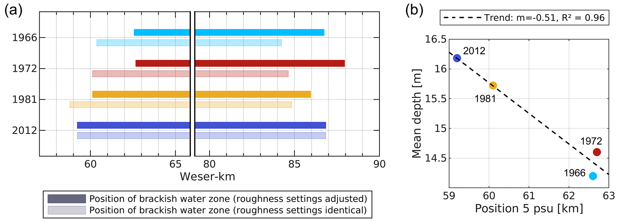
Figure 7 The left diagram (a) shows the effect of topography and roughness variation on the mean position of the brackish water zone (the stretch between the 5 psu and 20 psu isohalines along the navigation channel, see Fig. 1). The dark colours represent simulations with adjusted roughness settings; the light colours represent simulations with identical roughness settings. Forcing is identical. On the right (b), the mean position of the 5 psu isohalines in the simulations with adjusted roughness settings is displayed in relation to the mean depth of the navigation channel between Weser-km 40 to 100.

4.5 Relevance of roughness calibration for the examination of saltwater intrusion in different scenarios

To evaluate the impact of the roughness calibration on the results, we compared simulations with different model topographies but with identical roughness settings (settings of hindcast model 2012) with the simulations with individually adjusted roughness settings, as obtained by calibration of the respective hindcast models. When the roughness settings are identical, there is no clear trend regarding shifts in saltwater intrusion length between 1966 and 2012. In scenario 1981, salinity values in the Lower Weser are slightly larger than in 2012; in scenario 1966 and 1972, values are slightly lower (see Fig. 7a). However, simulations with identical roughness settings do not adequately reproduce tidal energy, e.g. the tidal range in 1981 is larger than in 2012 contrary to observations. The erroneously increased tidal range exceeds the effect of changes in other processes, so that the limit of saltwater intrusion shifts seawards, and not landwards, between 1981 and 2012.

4.6 Impact of topography changes on salt transport processes

Topography changes can influence tides in the estuary, e.g. the tidal range may increase due to increasing depths. For the Weser estuary, this effect is confirmed in the simulations with identical forcing. For example, the tidal range at Weser-km 60 increases from 3.65 m in 1966, 3.67 m in 1972, 3.86 m in 1981, to 3.88 m in 2012. This affects saltwater intrusion. Along with tidal effects, other salt transport processes such as the estuarine circulation can change through topography changes. In order to disentangle individual processes, the salt flux through a characteristic cross section was analysed in scenario simulations of 1966, 1972, 1981, and 2012. The scenarios contain identical boundary values but different topographies and roughness settings (see Table 1, scenario study).

We decomposed the total salt flux through a cross section in the Lower Weser (Weser-km 60, see Fig. 1) over the period of one spring–neap cycle for each scenario into barotropic flux, tidal pumping flux, and the estuarine exchange flow (see Sect. 3.5.2). Results of all scenarios (see Fig. 8) indicate that salt is mainly transported into the Weser estuary through tidal pumping. There is also a clear contribution from the estuarine exchange flow, especially in the scenarios 1981 and 2012. Exchange flow and tidal pumping are counteracted by the barotropic flux, which transports salt seawards.

The results indicate that the landward as well as seaward salt transport increased due to the topography changes between 1972, 1981 and 2012. Between 1972 and 1981, the examined cross section was directly affected by a deepening of the Lower Weser, which seems to induce an increase in estuarine exchange flow by more than 3-fold. At the same time, a minor increase in tidal pumping occurs and the barotropic flux increases. Between 1981 and 2012, the cross section is indirectly affected by deepening measures in the Outer Weser. The estuarine exchange flow component slightly decreases and there is an increase in tidal pumping and barotropic flux.

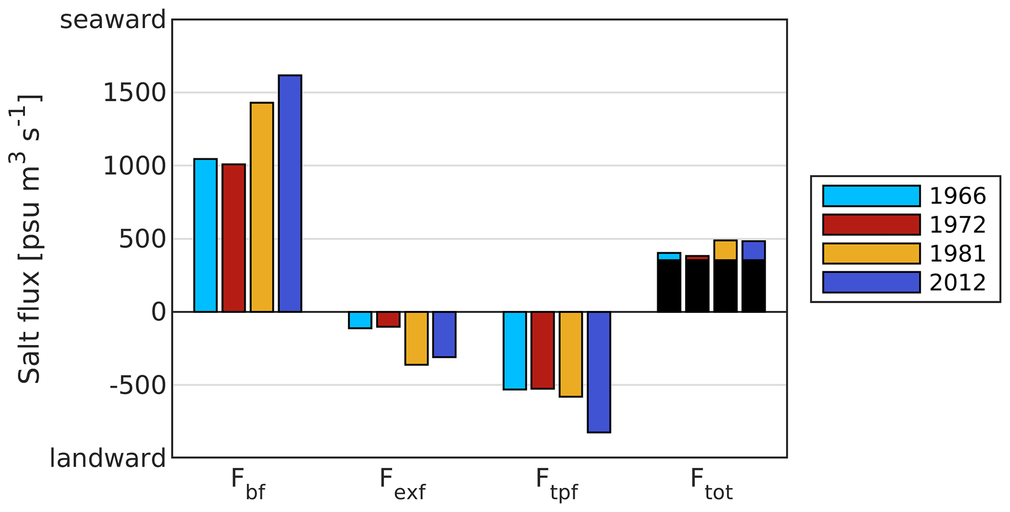
Figure 8 Salt flux through a cross section in the Lower Weser (Weser-km 60), calculated for the period of one spring–neap cycle based on simulations with identical forcing, but different topography and roughness settings. The barotropic flux F_bf, the estuarine exchange flow component F_exf, the tidal pumping component F_tpf, and the total flux F_tot are displayed. The contribution of the river discharge to the total salt flux is highlighted in black.

Note that the total salt flux contains the effect of the river discharge. The river discharge is constant in all scenarios with a salinity of 1.2 psu (see Table 1, scenario study), contributing to the total salt flux with a seaward salt flux of 300 m³ s⁻¹ ⋅ 1.2 psu = 360 psu m³ s⁻¹. The remaining total flux reflects variability in salt storage, which is expected as the simulation is not in a steady state, i.e. the water level at the North Sea boundary contains both tidal components and surge.

5 Discussion

Saltwater intrusion is subject to high natural variability, and salinity measurements of the past decades are not always available or exhaustive. This makes it difficult to quantify the effect of anthropogenic measures based on measurements only. With numerical simulations, we analysed the impact of anthropogenic measures on saltwater intrusion in two ways: First, we evaluated saltwater intrusion in hindcast models of the hydrological years 1966, 1972, 1981, and 2012 and analysed it as a function of discharge. Second, we evaluated saltwater intrusion in a scenario study with identical boundary values.

In the model set-up, a key challenge was the lower frequency and coverage of historical measurements compared to the present state, i.e. for water level, salinity, and temperature (see Sect. 3.4). This can lead to differences in model accuracy and compromise the comparability of model results. In our case, a detailed validation of the historical models was not possible due to the lack of historical salinity measurements. With a systematic approach and equal treatment of the respective system states, wherever possible, we created consistency and minimized bias. For example, we generated boundary values of all models with identical methods and calibrated each model individually.

In our study, an individual calibration of roughness parameters proved essential (see Sect. 3.6). Without calibration, changes in sediments and bedforms and the effects of different resolutions of bathymetric data strongly influenced model results and led to false conclusions (i.e. seaward shift instead of landward shift due to topography changes between 1981 and 2012). It has to be noted that calibration is only possible if observational data are available to support a robust calibration. Recalibration with imprecise data of low resolution might even affect model results negatively. In addition, it might not always be necessary, depending on the representation of roughness and sediments and on the resolutions of bathymetric data and the grid. However, we recommend conducting a thorough evaluation of bathymetric data and, if needed and possible, calibration of each model when results of models with different topographies are to be compared.

The analysis of hindcast results showed that, at similar discharge conditions, there is a landward shift in the position of the brackish water zone between 1966–1981 and 1981–2012 (see Sect. 4.3). The exact distance of the shift depends on the discharge condition (see Table 4). When comparing saltwater intrusion at times with a discharge of 300 m³ s⁻¹, there is a 2.4 km shift between 1966 and 1981 and a 1.8 km shift between 1981 and 2012. In the scenario study with identical boundary conditions, i.e. Q=300 m³ s⁻¹, the 5 psu isohaline shifts by 2.5 km between 1972 and 1981 and by 1 km between 1981 and 2012 (see Sect. 4.4). Both analyses show that anthropogenic measures in the Weser estuary led to an increase in the saltwater intrusion. This is in agreement with findings for other estuaries, where the navigation channel was also deepened (Andrews et al., 2017; Grasso and Le Hir, 2019; Ralston and Geyer, 2019). In the hindcast study, additional factors such as tides and salinity in the North Sea influence saltwater intrusion. In addition, the evaluation of saltwater intrusion depending on discharge does not account for adaptation time to changing discharge conditions. Nevertheless, results of both the hindcast study and the scenario study indicate an overall shift in the same range, i.e. 3.5–4 km. Measures in the Lower Weser, which were conducted during 1973–1978, had the highest impact. However, the exact extent of saltwater intrusion will also be influenced by factors not included in the model such as changes in tributaries, side channels, and the construction of waterways infrastructure.

The influence of discharge on saltwater intrusion follows the relationship $L\sim Q^{-\mathrm{0.15}}$ in our simulations (see Sect. 4.3). Thus, changes in discharge have a higher impact for low-discharge than high-discharge conditions, in agreement with previous studies (Kösters et al., 2014). Ralston and Geyer (2019) examined the relationship between discharge and saltwater intrusion in the Hudson River in idealized scenarios with different discharge conditions. For both, bathymetries representing the present state and the pre-development state, the sensitivity of the saltwater intrusion to discharge follows $L\sim Q^{-\mathrm{0.28}}$. The large difference from the sensitivity found in our study could be related to differences in bathymetry and transport processes between the estuaries. While saltwater intrusion into the Hudson is dominated by estuarine exchange flow, we show that the Weser is dominated by tidal pumping (see Sect. 4.6). Following Ralston and Geyer (2019), a change in the sensitivity of saltwater intrusion to discharge could indicate a change in salt flux mechanisms. We detect a significant but very small difference in the sensitivity in 1966 compared to 1981 and 2012 (see Sect. 4.3). However, the exact exponent depends on the definition of the saltwater intrusion length. Moreover, not only discharge, but also other influencing factors vary in the examined simulations, and lag times in the adjustment of saltwater intrusion to changed conditions were not considered in our analysis. Therefore, the small difference in sensitivity to discharge between 1966 and 1981 cannot be clearly attributed to a change in salt flux mechanisms.

The impact of anthropogenic measures on processes governing saltwater intrusion was further examined based on results of the scenario study (idealized forcing) (see Sect. 4.6). For all scenarios, a decomposition of the salt flux through a characteristic cross section in the Lower Weser was conducted according to Becherer et al. (2016). The salt flux was divided into contributions from barotropic flux, tidal pumping, and the estuarine exchange flow. Results indicate that salt flux in the Weser estuary is dominated by tidal pumping and barotropic flux. This also explains the result that saltwater intrusion is stronger during spring tides than during neap tides (see Sect. 4.1). By contrast, saltwater intrusion in estuaries dominated by estuarine exchange flow decreases during spring tides. Grasso and Le Hir (2019) found that the effect of the spring–neap cycle on saltwater intrusion can change if the governing processes in the estuary change. Even though our analysis was conducted for one cross section only, we expect that due to the channel-like geometry of the Lower Weser this is sufficient as a first characterization of the governing processes. However, we suggest a more complete characterization for further investigations, which includes analyses at different cross sections and different hydrological situations. A more extensive study disentangling the role of different processes in Weser estuary is currently being carried out by Marius Becker (personal communication, 4 July 2022).

The estuarine exchange flow through the cross section strongly increases between 1972 and 1981, while tidal pumping increases between 1981 and 2012. In both cases, this is outbalanced by a simultaneous increase of the barotropic flux. A possible interpretation could be that deepening measures in the Weser estuary locally induce an increase in estuarine exchange flow and globally induce an increase in tidal pumping. In addition, the shape of the estuary and the depth distribution are complex and the impact of a deepening measure depends on its location, meaning a deepening of the outer estuary such as between 1981 and 2012 has a different impact than a deepening of the inner estuary such as between 1972 and 1981. This aspect could be further explored in future studies, which should also include the analysis at different cross sections and an analysis of lateral processes. In the Outer Weser estuary, which is characterized by wide cross sections and a two-channel system (Gundlach et al., 2021), lateral variations could significantly influence salt transport processes (Wei et al., 2022). In addition, other decomposition methods could be tested (e.g. Dyer, 1974; Dronkers and van de Kreeke, 1986; Park and James, 1990; Hughes and Rattray, 1980).

6 Conclusions

Saltwater intrusion in the Weser estuary is highly variable and dependent on natural forcing factors, i.e. river discharge, as well as anthropogenic impacts, i.e. channel deepening. A systematic study of the effect of topography changes on saltwater intrusion was carried out to disentangle these overlapping influencing factors. This study used numerical models of four system states (1966, 1972, 1981, and 2012) with respective topographies to hindcast the historical development of saltwater intrusion (hindcast study) and examine the effect of anthropogenic measures (scenario study). The models were individually calibrated and validated to account for differences in sediments, bedforms, and the resolutions of underlying bathymetric data.

In the hindcast simulations, the influence of topography is overshadowed by the effect of other factors, particularly discharge. The salinity front is about 10 km more landward in 1972 and 2012 compared to the other system states, as the average discharge is almost double in these years. However, at similar discharge, a landward shift of the salinity front is indicated between 1966 and 1981 and between 1981 and 2012. This trend is confirmed in the scenario study. With identical boundary values (i.e. Q=300 m³ s⁻¹), the salinity front shifts landwards by about 2.5 km between scenario 1972 and 1981 and by about 1 km between scenario 1981 and 2012. It has to be noted that the exact distance by which the salinity front shifts depends on the discharge due to the nonlinear relation between discharge and saltwater intrusion. Analyses of the salt flux through a cross section in the Lower Weser indicate that the Weser estuary is dominated by barotropic flux and tidal pumping, while the estuarine exchange flow is of secondary importance in all scenarios.