Surface circulation properties in the eastern Mediterranean emphasized using machine learning methods

The eastern Mediterranean surface circulation is highly energetic and composed of structures interacting stochastically. However, some main features are still debated, and the behavior of some fine-scale dynamics and their role in shaping the general circulation is yet unknown. In the following paper, we use an unsupervised neural network clustering method to analyze the long-term variability of the different mesoscale structures. We decompose 26 years of altimetric data into clusters reflecting different circulation patterns of weak and strong flows with either strain or vortex-dominated velocities. The vortex-dominated cluster is more persistent in the western part of the basin, which is more active than the eastern part due to the strong flow along the coast, interacting with the extended bathymetry and engendering continuous instabilities. The cluster that reflects a weak flow dominated the middle of the basin, including the Mid-Mediterranean Jet (MMJ) pathway. However, the temporal analysis shows a frequent and intermittent occurrence of a strong flow in the middle of the basin, which could explain the previous contradictory assessment of MMJ existence using in-situ observations. Moreover, we prove that the Levantine Sea is becoming more and more energetic as the activity of the main mesoscale features is showing a positive trend.

1 Introduction

The Levantine Sea surface circulation is controlled by a complex mesoscale system composed of eddies, jets, and filaments interacting stochastically with each other (Özsoy et al., 1991). This basin lies on the easternmost part of the Mediterranean, bounded by the Cretan Archipelago, Asia Minor to the north, the Middle East to the east, and northeastern Africa to the south. One of the main reasons behind its complex dynamic is its peculiar bathymetry, characterized by the presence of the Herodotus Abyssal Plain at 3000 m depth. It is a deep and large sub-basin located in the southern part of the Levantine basin between Libya and Egypt. However, other shallower sub-basins also exist, such as the Lattakia, Cilicia, and Antalya sub-basins. To the south of Cyprus, there is a notable presence of the Eratosthenes Seamount, whose summit is about 700 m deep. Furthermore, the mesoscale activity of the Levantine basin has a continuous and direct impact on physical and biogeochemical water properties, where, for example, currents transport chemicals originating from rivers and nutrient-rich waters into the oligotrophic open sea (Taupier-Letage et al., 2003; Lehahn et al., 2007; Escudier et al., 2016). Although the mesoscale activity is highly evolving in the eastern Mediterranean, some of the mesoscale features are almost permanent and appear as separate building blocks (Matteoda and Glenn, 1996; Rio et al., 2007). These well-defined blocks include the anticyclonic eddies of Mersa Matruh, Shikmona, and Cyprus and the cyclonic Rhodes gyre (see Fig. 1a) (Amitai et al., 2010; Larnicol et al., 2002; Gerin et al., 2009; Menna et al., 2012).

Several studies have aimed to characterize the surface dynamics of this basin, such as Hamad et al. (2005) or Taupier-Letage (2008), which provided a descriptive analysis of the eastern Mediterranean sea surface currents using sea surface temperature images from satellites. Moreover, by using altimetric data, the long-term averaged mean dynamic topography (MDT) (Amitai et al., 2010), current flow kinetic energy variability (Pujol and Larnicol, 2005; Menna et al., 2012), and eddy tracking (Mkhinini et al., 2014) allowed for the analysis of the long-term surface current and long-lived eddies. However, these studies showed average patterns, mainly emphasizing existing and permanent eddy activities, with less focus on interannual variability or other patterns, such as jets and weak flows.

Additionally, there is a previous contradictory assessment of the presence of the Mid-Mediterranean Jet (MMJ, see Fig. 1a) (Ciappa, 2021), which is described as a surface current meandering across the Levantine Sea. Some authors consider the MMJ as an artifact caused by the deviation of the coastal Atlantic Water (AW) driven from one eddy to another. In other terms, it is the result of the paddle-wheel effect due to the high mesoscale activity across the eastern Levantine basin. Indeed, no remarkable jets were observed during the Mediterranean Forecast System (MFS) program (Manzella et al., 2001), during expendable bathythermograph (XBT) campaigns (Horton et al., 1994; Zervakis et al., 2003), by the sizable drifter data set released during the EGYPT/EGITTO program between September 2005 and July 2007 (Millot and Gerin, 2010; Gerin et al., 2009), or even when using high-resolution numerical models (Alhammoud et al., 2005). Nevertheless, other observational studies have shown a clear across-flow pattern in the middle of the basin with an average speed ranging between 10 and 19 cm s⁻¹ (Amitai et al., 2010; Poulain et al., 2012). More recently, sea surface temperature (SST) anomaly satellite images, drifter tracks, and the geostrophic currents computed from the satellite absolute dynamic topography (ADT) fields showed an occasional MMJ flowing toward the north of the Lebanese coast between 2016 and 2017 (Mauri et al., 2019). In Ciappa (2021), the investigation of SST and altimetry images between 2000 and 2015 considered that the MMJ is triggered by the surface cold water pushed by a northerly wind, reaching the northern periphery of the Libyan and Egyptian coasts, and the high vorticity off the Libyo-Egyptian Eddies (LEE) that injects the MMJ into the middle of the eastern Levantine basin.

Currently, satellite altimetry is a widely used observational tool for analyzing sea surface physical dynamics and mesoscale activity and provides a continuous coverage for more than 25 years (Ducet et al., 2000; Bosch et al., 2014; Fu and Cazenave, 2000; Hamlington et al., 2013; Willis, 2010; Abdalla et al., 2021). When such a large data set is available, machine learning methods could be applied efficiently to characterize the surface circulation and identify patterns. One efficient method is the use of a self-organizing map (SOM, (Kohonen, 2013)), a high-performance unsupervised clustering algorithm applied in different fields to classify and extract features. In the oceanography, the SOM was applied to characterize the interannual, seasonal, and event-scale variability of wind and SST patterns (Richardson et al., 2003) and phytoplankton pigment variability (El Hourany et al., 2019). The tool was also efficient for the characterization of the coastal areas by combining high-resolution numerical models with radar observations (Ren et al., 2020) or radar with an acoustic Doppler current profiler (ADCP) data set, such as in the West Florida Shelf (Liu et al., 2007) or the Long Island Sound tidal estuary (Mau et al., 2007). In the Mediterranean, SOM was applied in the Adriatic Sea using the high-frequency (HF) radar measurements (Mihanović et al., 2011) and in the Strait of Sicily using 46 years of a high-resolution model (Jouini et al., 2016). This approach allowed for the decomposition of the surface circulation in the Sicily Channel into modes reflecting the variability of the circulation in space and time at seasonal and interannual scales. SOM was also able to provide a prediction of the surface current in the shallow coastal area (Kalinić et al., 2017) and to identify phytoplankton functional types in the Mediterranean Sea using a bioregionalization approach (El Hourany et al., 2019; Basterretxea et al., 2018).

In light of the major gaps in characterizing the surface currents of the Levantine Sea and previous contradictory assessments, the present paper aims to improve the understanding of its surface dynamics and mesoscale structures using machine learning techniques. To reach this aim, we adapt the neural network clustering method, the SOM method, and the hierarchical ascendant classification (HAC) method as used in (Jouini et al., 2016), which will allow for the decomposition of Levantine Sea surface velocity between 1993 and 2018 into different regimes for the estimation of possible seasonal and interannual variations of the main mesoscale features. We also provide a possible explication of the reasons behind the contradictory assessment of the MMJ's existence. We finally show the vorticity variation in the basin and the main factors affecting the apparition and persistence of the mesoscale features.

The paper is structured as follows. We start by presenting the data and the clustering method used to obtain the different clusters in Sect. 2. Additionally, we present the approach used for the delimitations of the main mesoscale features zones. Results of decomposing the circulation are presented in Sect. 3 and discussed in Sect. 4. A conclusion is presented in Sect. 5.

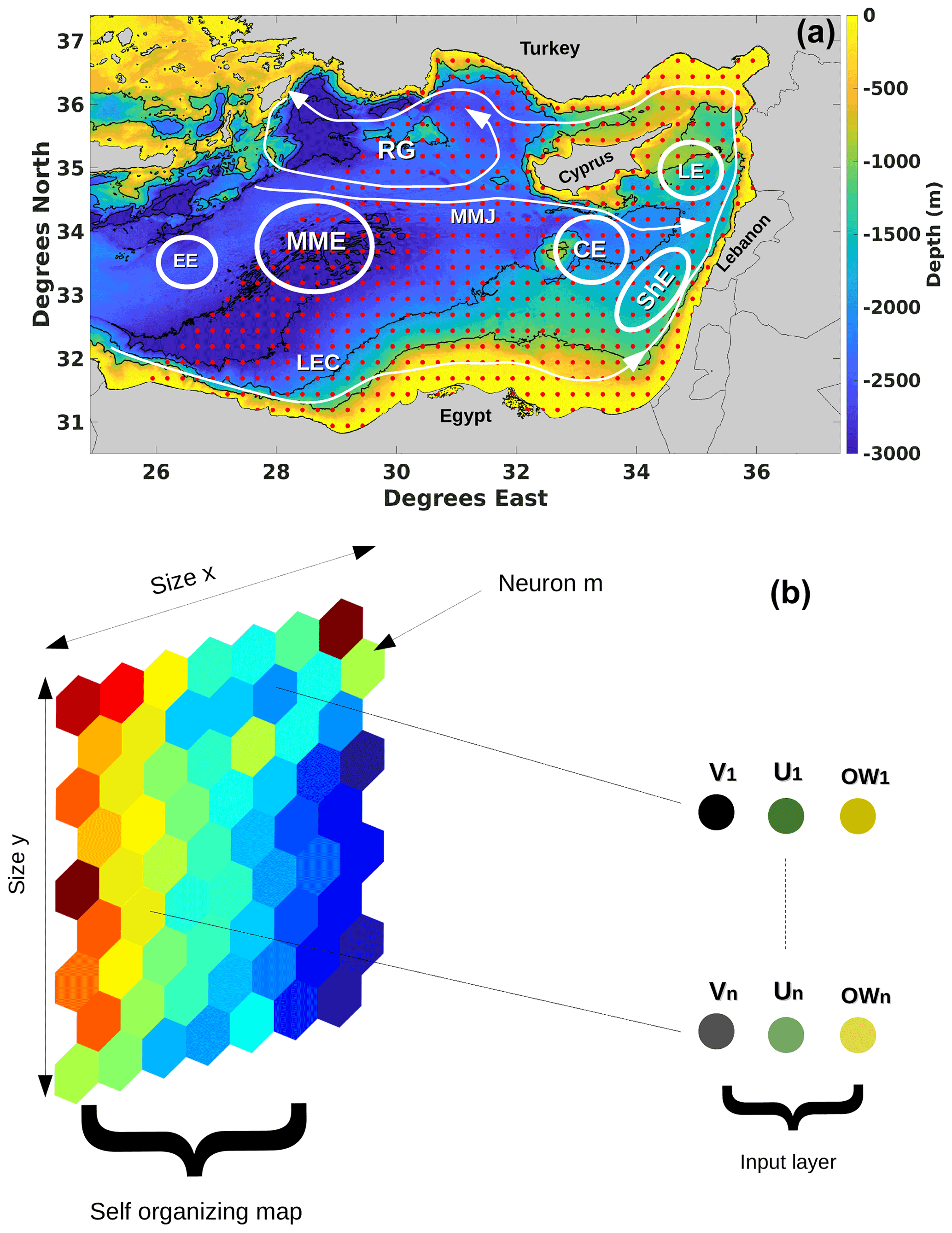
Figure 1 (a) A schematic representation of the main structures present in the Levantine basin (RG: Rhodes Gyre; LE: Lattakia Eddy; EE: Egyptian Eddy; LEC: Libyo-Egyptian Current; MMJ: Mid-Mediterranean Jet; MME: Mersa Matruh Eddy (also known as Herodotus Trough eddies); CE: Cyprus Eddy; ShE: Shikmona Eddy; LE: Lattakia Eddy). All elements are placed in the context of a bathymetry map. The red dots represent the coordinates of the grids providing the input data for the SOM. Each red dot (n) is composed of U and V components and the Okubo–Weiss (OW) parameter. (b) A schematic representation of the SOM method: the input layer obtained from the input data and the adaptation layer composed of n neurons automatically associated in an orderly fashion. Each neuron represents a set of U, V, and OW that represents similarities.

2 Data and methods

This section presents the data and methodology used for the restitution of the surface circulation regimes based on the concept of SOM and HAC methods. We then present the approach used to divide the basin into six geographical sub-regions (or boxes) that include the different mesoscale features.

2.1 Altimetry

The altimeter satellite gridded sea level anomaly (SLA) is estimated by optimal interpolation, merging the measurement from the different altimeter missions available. This product is processed by the DUACS (Data Unification and Altimeter Combination System) multi-mission altimeter data processing system. It processes data from all altimeter missions: Jason-3, Sentinel-3A, HY-2A, Saral/AltiKa, Cryosat-2, Jason-2, Jason-1, T/P, ENVISAT, GFO, and ERS1/2. To produce reprocessed maps in delayed time, the system uses the along-track altimeter missions from products called $\text{SEALEVEL}{\mathit{\_}}^{\ast }\text{PHY}\mathit{\_}\text{L3}\mathit{\_}\text{MY}\mathit{\_}{\mathrm{008}}^{\ast }$. The SLA computation provides the absolute dynamic topography (ADT) and the surface geostrophic currents. The velocity field spatial resolution is $\mathrm{0.125}{}^{\circ }\times \mathrm{0.125}{}^{\circ }$ (available on http://www.aviso.altimetry.fr/duacs/, last access: 20 September 2021).

The daily geostrophic surface velocity fields between 1993 and 2018, from the Herodotus Abyssal Plain and until the easternmost part of the Levantine sea, form the input layer of the SOM. In addition to the zonal and meridional components of the geostrophic velocities, the fluid parameter of Okubo–Weiss (OW) is included in the input layer (see Fig. 1b). OW measures the relative importance of deformation and rotation at a given point. Positive OW values indicate strain-dominated regions, while negative OW indicates a vortex-dominated region. Accordingly, OW is a physical criterion widely used in the methods of eddy detection.

$\text{OW}=s_{\text{n}}^{\mathrm{2}}+s_{\text{s}}^{\mathrm{2}}-w^{\mathrm{2}}$, where s_n and s_s are the normal and the shear components of strain and w is the relative vorticity of the flow defined, respectively, by

$$\begin{array}{}\text{(1)}& s_{\text{n}}={\displaystyle \frac{\partial U}{\partial x}}-{\displaystyle \frac{\partial V}{\partial y}},s_{\text{s}}={\displaystyle \frac{\partial V}{\partial x}}+{\displaystyle \frac{\partial U}{\partial y}},w={\displaystyle \frac{\partial V}{\partial x}}-{\displaystyle \frac{\partial U}{\partial y}}.\end{array}$$

2.2 The self-organizing map (SOM)

SOM is an unsupervised neural network method used for data visualization. It projects higher-dimensional data into lower-dimensional space by leveraging topological similarity properties. By this method, multidimensional data are clustered into neurons automatically associated into an orderly organization, where similar neurons are adjacent, and the less similar neurons are situated far from each other in the grid. This way allows for obtaining an insight into the topographic relationships of the initial data set (Kohonen, 2013).

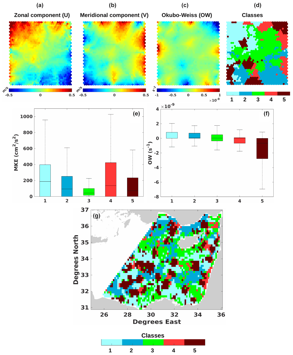
Figure 2 Panels (a–c) reveal the topological maps of three variables, U, V, and OW, respectively, using an SOM after the training phase. Each map shows the recorded values by each neuron for the three variables. The resulting clusters obtained from the SOM and HAC method are shown in (d). Mean kinetic energy (MKE) and OW values of each cluster are shown in the boxplots in (e) and (f), respectively. A random example (25 June 1998) of the decomposition of daily surface currents into the five clusters is presented in (g).

The SOM is structured in two layers: the input layer (in our case, a 3-D input layer composed of the zonal and meridional components and the Okubo–Weiss parameter) and the resulting neuron grid. Each neuron, representing a cluster with data presenting common characteristics, is associated with a referent vector obtained from a learning data set. Each vector of the input layer will be attributed to the neuron with the closest Euclidean distance to the referent vector. This referent vector is called the best matching unit (BMU), and its associated neuron is the “called” winning neuron. The determination of the referent vectors and the topological order of the SOM maps is done by minimizing the cost function

$$\begin{array}{}\text{(2)}& {\mathcal{J}}_{\text{SOM}}^T(\mathcal{X},W)=\sum _{zi\in D}\sum _{c\in \text{SOM}}{\text{K}}^T\left(\mathit{\delta }\right(c,\mathcal{X}\left(z_{\text{i}}\right)\left)\right)\left|\right|z_{\text{i}}-w_c|{|}^{\mathrm{2}},\end{array}$$

where c∈SOM represents the neuron index in the SOM, 𝒳(z_i) represents the allocation function that assigns each element z_i of the input D to the corresponding referent vector $w_{\mathcal{X}\left(z_{\text{i}}\right)}$, δ(c,𝒳(z_i)) represents the discrete distance on the SOM between a neuron c and the neuron allocated to observation z_i, and K^T is a kernel function parameterized by T (where T stands for temperature in the scientific literature dedicated to SOM) that weights the discrete distance on the map and decreases during the minimization process. During the minimization of the cost function, the topological order is preserved, and thus the more similar neurons are adjacent and the less similar neurons are situated far from each other. To provide an equal-weight distribution of the input parameters, the variables were normalized with their variances. Several tests were conducted to determine the optimal size of the SOM map giving the best representation of the data. These tests were based on the capacity of each map to reproduce the initial data space of our input data with the least error possible. Based on this choice, we opted for a large SOM map of 1400 neurons.

After the training phase, the SOM is well organized where there is a gradient of zonal and meridional velocities. This distribution of U (Fig. 2a) and V (Fig. 2b) reflects the OW variation well (Fig. 2c). The OW in SOM shows clusters of intense positive or negative values. These extreme values represent the characteristics of a vortex (positive) or strain (negative) dominance.

Figure 3 (a) Mean dynamic topography (MDT) between 1993 and 2018 in the eastern Levantine basin. (b) The standard deviation of the absolute dynamic topography (ADT) for the same period. Both include the names and borders of the six delimited sub-regions or boxes (MME: Mersa Matruh Eddy; CE: Cyprus Eddy; Nile; Shik: Shikmona Eddy; Bei: Beirut; AMC: Asia Minor Current).

2.3 HAC method

The SOM allowed for classifying the velocity field into neurons that represent the different circulation patterns of the targeted grid based on U, V, and OW. To simplify the representation of the physical processes obtained from the different situations captured by each neuron, we applied the HAC to group these neurons into a reduced number of clusters. HAC is a cluster analysis that seeks to build a bottom-up hierarchy of clusters. From the initial partition containing the neuron groups of the SOM map, two neurons of the same neighborhood were clustered at each iteration. The used criterion was Ward's minimum variance method, which provides a partition that minimizes the within-cluster inertia (Randriamihamison et al., 2021) while respecting the topological organization. As a result, the neurons were separated into five different clusters (see Fig. 2d). Consequently, clusters 4 and 5 (denoted as C4 and C5) were characterized by a negative OW, compared to positive OW for C1 and C2, while C3 had an average OW of 0. MKE boxplots of the neurons in each cluster show that C3 had the weakest flow intensity, while C4 and C1 represented the highest MKE intensities, followed by C2 and C5 (Fig. 2e and f). In summary, C1 and C2 are clusters of strong flow with high vorticity (high MKE and positive OW), C4 and C5 are clusters of strain-dominated strong flow (negative OW and high MKE), and C3 is the cluster of the weakest velocities.

2.4 Studied area

To analyze the activity of the most dominant features in the Levantine basin, we targeted the area from the Herodotus Abyssal Plain until the easternmost part of the Mediterranean Sea. The Mersa Matruh Eddy (MME) (see Fig. 1) is an eddy generated by the coastal instabilities near the eastern Libyan and Egyptian coasts. These eddies drift seawards while being guided by the 3000 m isobath. Indeed, the 3000 m Herodotus Plain traps and prevents the coastal vertically extended eddies from propagating further to the east, thus causing an accumulation of these eddies in this area (Alhammoud et al., 2005; Elsharkawy et al., 2017). MME is one of the most dominant mesoscale features in the eastern Mediterranean, where their mean kinetic energy exceeds 300 cm² s⁻² (Menna et al., 2012). In the easternmost part of the basin, the Shikmona Eddy (ShE) system (see Fig. 1) represents another complex system composed of several cyclonic and anticyclonic eddies with varying sizes, positions, and intensities (Gertman et al., 2007; Menna et al., 2012; Mauri et al., 2019). Similar to MME, ShE is an area where previously formed eddies tend to accumulate and/or merge (Hamad et al., 2005). Another important mesoscale feature existing in the eastern part is the Cyprus Eddy (CE) (see Fig. 1). It is an intense dynamic feature occurring in the open sea. Unlike the MME and ShE, eddies are formed in this area and do not accumulate (Zodiatis et al., 2005). We should note that other mesoscale structures exist in the eastern Levantine basin but are less frequently observed. Among these, we mention the “Lattakia Eddy” (LE) taking place between Cyprus and Syria. LE is a cyclonic eddy generated by the interaction of the northward current along the Lebanese and Syrian coasts with a Mid-Mediterranean Jet (Zodiatis et al., 2003) or between ShE and the coastline (Hamad et al., 2005) or generated by the topography (Gerin et al., 2009).

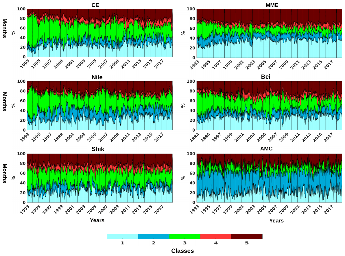
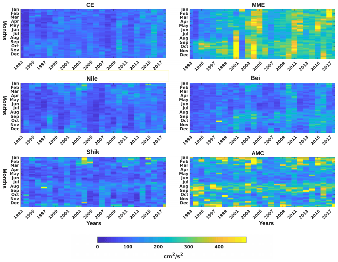
Figure 4 The daily variation of each cluster frequency in each of the selected boxes between the beginning of 1993 and late 2018. This frequency variation reflects the percentage of pixels that were affected by each of the five clusters in a designated box.

2.4.1 Definition of main mesoscale features regions

The eddies usually reveal elevations (anticyclones) or depressions of the sea surface. Accordingly, and after decomposing the Levantine surface circulation (e.g. Fig. 2g), we delimited the main mesoscale eddies areas by using an approach similar to that used by (Barboni et al., 2021) by computing the mean dynamic topography (MDT) map obtained from averaging absolute dynamic topography (ADT) for over 26 years between 1993 and 2018. Additionally, we used the resulting standard deviation to detect highly variable areas. In Fig. 3a, the MDT show several eddy structures consistently present in the basin. The positive MDT values, revealing anticyclonic circulation structures, were around the depth of the Eratosthenes Seamount and the Herodotus Abyssal Plain. On the other hand, negative MDT values, hosting cyclonic circulation, were observed between Cyprus and Asia Minor and in the Shikmona area between the south of Lebanon and Egypt. The representation of MDT standard deviation (B) shows similar mesoscale structures, with two additional active zones observed offshore from the Lebanese coast and west of the Eratosthenes Seamount. Based on these results revealed by the average and the standard deviation of the dynamic topography, we divided the basin's mesoscale activity into several boxes: the Beirut area off the Lebanese coast (Bei), the Cyprus Eddy that includes the Eratosthenes Seamount (CE), the Mersa Matruh Eddy above the Herodotus Plain (MME), the Nile, the Shikmona Eddy (Shik), and the Asia Minor Current area (AMC).

3 Results and discussion

In this section, we present the results of decomposing the surface circulation of the Levantine basin into a daily time series of five clusters obtained by the HAC and SOM methods.

Figure 5 The daily dominant cluster in each box from 1993 and 2018.

3.1 Temporal variation

The frequency variation of the five clusters in each of the selected boxes, i.e., Bei, Shik, MME, AMC, Nile, and CE, is seen in Fig. 4. This frequency variation reflects the percentage of pixels assigned to each of the five clusters in a designated box. As a result, except for C4 in the AMC, all the clusters permanently occurred, with different proportions highly variable with time in each box. Moreover, cluster frequency significantly varies from one box to another.

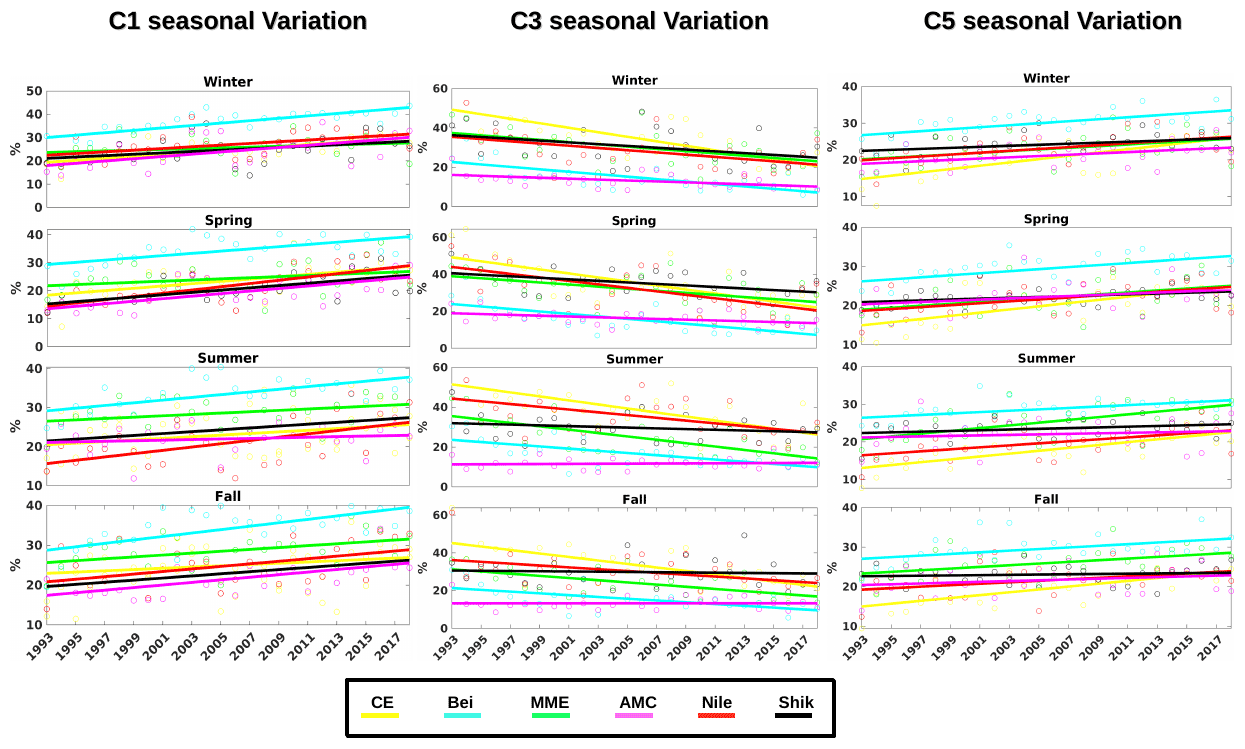
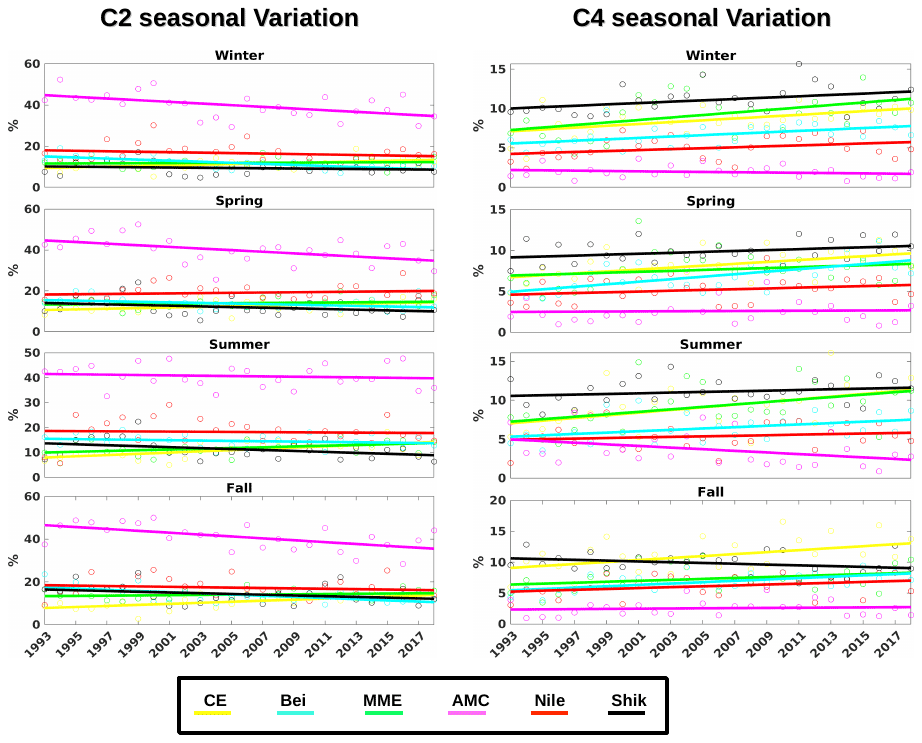
Figure 6 The seasonal variation of the C1 (high kinetic energy), C5 (high vorticity), and C3 (low kinetic energy and low vorticity) average in each box and their resulting linear regression.

Although clusters of strain-dominated flow (C1 and C2) were not frequent everywhere, C1 and C2 were frequently observed in MME and AMC, respectively, during the entire period. Such a high frequency occurred at the expense of other clusters, especially the cluster of weak flow C3, which was less observed in these two boxes. Regarding the vortex-dominated clusters (C4 and C5), C5 was the most frequent. C4 was quasi-absent in AMC and scarcely existed in the other boxes. When comparing between boxes, C5 was most frequent in the MME. Overall, all the cluster occurrences fluctuated greatly over time. To better analyze such a frequency variations, we presented the daily dominant cluster in each box in Fig. 5. On the one hand, C3 was the main cluster in CE, Nile, Bei, and Shik boxes. Moreover, between 1993 and 2000, C3 dominated CE almost exclusively. On the other hand, C3 dominance was rare or quasi-nonexistent in the MME and AMC, where instead C1 and C2, respectively, were the most frequent clusters. While C2 dominance was not observed in MME, an increasing periodic C1 domination was observed in AMC, starting from 2000. C5 was frequently dominating all the boxes, albeit intermittently. This dominance was rare in the CE, Nile, and AMC, compared to the MME, Bei, and Shik. Indeed, in these last three boxes, C5 dominance was frequent and showed a long lifetime that could last for several months, such as observed in Bei in 2003 and 2014 and Shik in 2005.

These results showed that MME and AMC are two zones of a special regime of flow. This latter zone is represented by clusters of intense current, the so-called C1 and C2. The other boxes are zones of relatively weaker currents. In all the boxes, there were sporadic events of intense eddy activity, exhibited by the intermittent periods of C5 dominance.

The daily mean kinetic energy of the mean flow per unit of mass (MKE) computed in each box (see Fig. A1 in the Appendix) shows that the lowest MKE values were observed in the boxes where C3 dominated the most (CE, Nile, Shik, and Bei). In these boxes, MKE values were less than 150 cm² s⁻². On the other hand, the highest values were in AMC and MME, with values consistently exceeding 300 cm² s⁻². Hence, the boxes dominated by C1 and C2 had MKE values that were 2 times higher than those observed in boxes dominated by C3.

The tendency of the dominant cluster could change with time, where previous results show, for example, that C5 was rare in Bei before being more frequently observed as a dominant cluster between 1993 and 1997. Figure 6 shows the seasonal variation of the C1, C3, and C5 average frequencies in all the boxes between 1993 and 2018. The general trend of C5 frequency increases over time. The most intense C5 positive tendency was in MME, where C5 increased by 10 % in 26 years. In all the seasons, the C5 frequency average in MME increased from 25 % in 1993 to 35 % in 2018. There was a similar increase in all the seasons in the Bei, MME, and Nile boxes. The weakest increasing tendency was in AMC and Shik. In terms of seasonality, there was no significant difference in C5 frequency between seasons, except in CE, where in summer and fall the values were higher, with values closer to the MME. MME registered the highest seasonal average frequency of C1, meaning that this box is the most dominant in terms of intensity and vorticity (C5 and C1). In terms of trends, C1 showed similar results to C5. The MME and Nile boxes showed the sharpest increases, followed by AMC, Nile, CE, and Bei, while C3 was continuously decreasing in all the boxes.

These results show that the activity of the dominant mesoscale is increasing with time. Previous altimetric data observations from 1993–2003 revealed increasing variability of the Mediterranean Sea activity that is maximal in the Levantine Sea, especially in the Mersa Matruh area, where increasing energetic structures were observed (Pujol and Larnicol, 2005). Studies have discovered evidence that eddies are becoming more energetic. This increase was related to several reasons, such as the changes in winds or large-scale horizontal temperature gradients or the changes in the shear of the ocean currents (Martínez-Moreno et al., 2021). This current evolution is well highlighted where C3 is being progressively replaced by C1. Nevertheless, we should not exclude the impact of the altimetry increasing accuracy in describing the surface circulation, with an increasing number of satellite tracks in both time and space. Satellite along-track sampling accurately estimates the sea surface height (SSH) from which the surface circulation is derived (Ducet et al., 2000). The interpolation of the gaps could lead to the underestimation of the mesoscale features. However, with the increasing number of satellites over time, the merging of altimeter missions provides a better description of the mesoscale activity (Pascual et al., 2006; Amores et al., 2019). In terms of seasonality, there was no significant difference in C5 frequency between seasons, except in CE, where in summer and fall the values were higher, with values closer to the MME. Although previous studies have mentioned that eddies in MME are mainly formed in summer and spring (Hamad et al., 2005; Mkhinini et al., 2014), there was no clear seasonality of C5 frequency. This is explained by the frequent eddy apparitions and their relatively long lifetime. Consequently, eddies permanently occur in the MME box (Taupier-Letage, 2008).

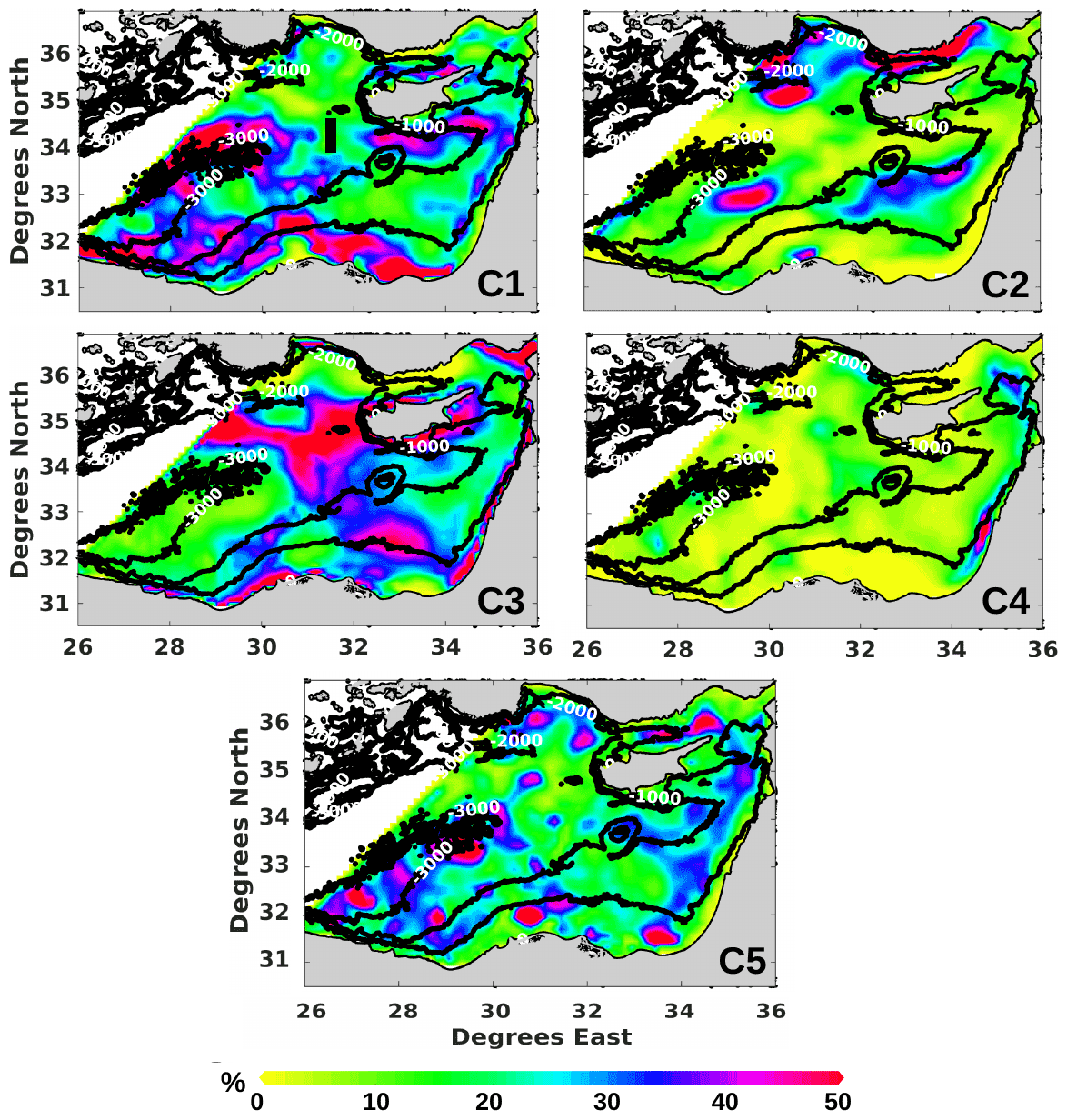
Figure 7 Percentage of C1, C2, C3, C4, and C5 occurrence between 1993 and 2018, superimposed onto the main bathymetric iso-lines of −1000, −2000, and −3000 m. The dark line in the C1 subplot shows the position of the Hovmöller diagram in Sect. 3.3.

It should be mentioned that C2 and C4 did not show a clear tendency. However, C2 was only significantly present in AMC with values around 40 %, while in all other boxes the frequency was less than 20 % (see Fig. A2 in the Appendix).

3.2 Spatial analysis

The spatial variation of clusters' frequencies is shown in Fig. 7. The intensity of the along-slope coastal flow showed a spatial variability. Indeed, the high kinetic energy clusters, C1 and C2, frequently occurred off the Libyo-Egyptian coast and between Turkey and Cyprus, respectively, while the weak current cluster, C3, dominated the easternmost part of the basin. The C5 predominance is mostly situated in the western part, revealing that the mesoscale activity is more intense in that area. No clear jet was observed in the middle of the basin, including the MMJ pathway, where C1 dominance was disconnected by high C3 occupancy between 30 and 32^∘ E (see C1 in Fig. 7).

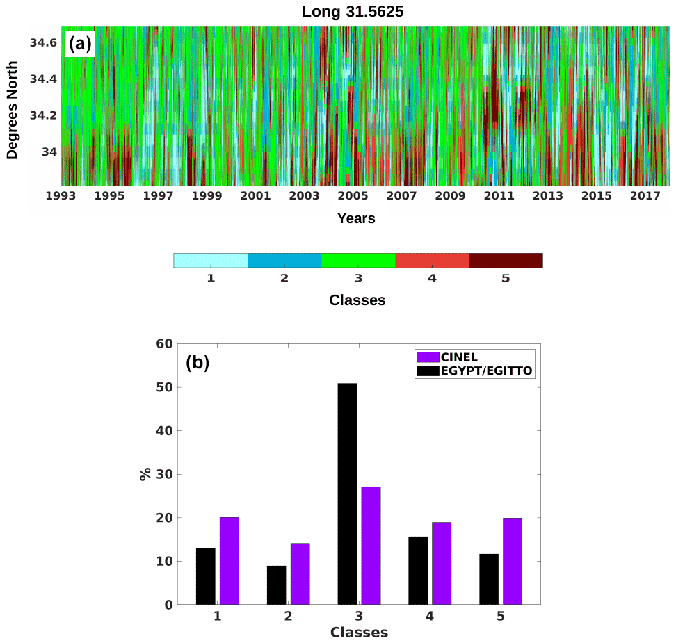
Figure 8 (a) Hovmöller diagram of daily cluster variation along the MMJ potential pathway at 31.5^∘ E. The resulting cluster frequencies during the EGYPT/EGITTO (September 2005–July 2007) and CINEL campaigns (September 2016–August 2017) are shown in (b).

3.3 Mid-Mediterranean jet (MMJ)

To further investigate the time evolution of the potentially existing MMJ, we present a Hovmöller diagram in Fig. 8a (along 31.5625^∘ E) that shows the temporal variation of the clusters across its potential path. The longitude selection was based on the previous results showing an area dominated by weak flow cluster C3 in the MMJ potential pathway between the Eratosthenes Seamount and the coast of Cyprus (see C1 frequency in Fig. 7). Although there was frequent C3 domination, there were years where clusters revealing higher kinetic energy (KE) were frequently occurring, such as C1 in 2015 or C5 between 2013 and 2014. An example of this variation is presented in Fig. 8b, which shows the cluster frequency distributions during the EGYPT/EGITTO (September 2005–July 2007) and CINEL campaigns (September 2016–August 2017) that provided in situ drifter observations in the MMJ potential pathway. During the EGYPT/EGITTO campaign, C3 frequency was more than 50 %, and the other clusters did not exceed 15 %, while during the CINEL campaign, clusters of stronger KE increased at the expanse of C3, decreasing to 27 %. All of these results reveal that the MMJ is present in the middle of the basin, but it is only present sporadically and is not one of the most remarkable features, and strong flow clusters were frequently observed here but were masked by C3, the dominant cluster in this area. In Millot and Gerin (2010), the drifter data set used from the EGYPT/EGITTO campaign showed no distinct jet between 2005 and 2007, a period of C3 domination. On the other hand, in Mauri et al. (2019) the drifter tracks showed a clear MMJ crossing the basin from west to east between late 2016 and 2017, a period when there was a sharp shift in C3 frequency, decreasing by more than half compared to EGYPT/EGITTO. The Hovmöller diagram also showed that MMJ variability was without any seasonal or periodic nature, in agreement with Ciappa (2021).

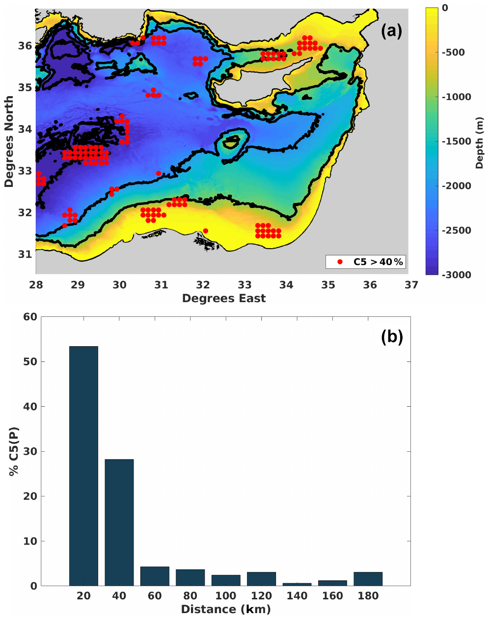
Figure 9 (a) The red dots show the positions of C5P, which are the pixels where C5 existed more than 40 % of the time. The dark line represents the main bathymetric iso-lines (1000, 2000, and 3000 m). (b) The variations of C5P frequency compared to their closest distance with these iso-lines.

3.4 Vortex-dominated cluster analysis

Both C4 and C5 are vortex-dominated clusters. However, the previous results showed that C4 is a peripheral cluster that is scarcely observed, dominating only very few pixels close to the coast. C5 was the main cluster that mainly reflected the eddies' presence. Here we present a more detailed analysis of the C5 evolution that reveals eddy activity in the Levantine Sea.

Figure 9a shows the spatial distribution of C5, whose occurrence exceeded 40 % (C5P). The highest persistent C5P number was at the borders of the Herodotus Plain. In addition, another group of C5P occurred in areas of the extended continental shelf, more precisely the shelf located offshore from Egypt and between Cyprus and Turkey in the northern part of the basin. A small number of C5P followed the bathymetric isobath of 1000 m in the western part of the basin. On the other hand, C5P was absent in the eastern part of the Levantine Sea. In Fig. 9b we present the variation of C5P numbers regarding their distances to the closest main bathymetric structures (iso-lines of 1000, 2000, and 3000 m). More than 80 % of C5P were located at a distance less than 60 km from these main features. In the zones of extended continental shelf, such as offshore from the Libyo-Egyptian coast, there is a strong flow dominated by C2 and C1. Previous studies have shown that a current becomes unstable when it is wider than the bathymetry. Thus, it presents favorable conditions for eddy formation (Wolfe and Cenedese, 2006). The C5P absence off the Lebanese coasts is explained by the tight continental shelf being almost absent. Indeed, the weak current dominated by C3 near the coastline is not strong enough to permanently create instabilities. The group of C5P observed in MME is due to the impact of the Herodotus Abyssal Plain. The vertically extended eddies pinch off from the coast and propagate to the east before being trapped, thus accumulating eddies (Alhammoud et al., 2005; Elsharkawy et al., 2017). These results show that the main bathymetric features could potentially influence eddy creation and persistence in the Levantine basin.

Figure 10 (a) The average velocity field obtained before (blue) and after assimilating (red) the drifters' trajectories represented by the grey lines, circulating in CE from the start of March until late July. (b) The percentage of pixels assigned to the clusters from 1 to 5 before (dark bars) and after assimilation (colored bars).

4 The effect of assimilation on the clustering

Because of the coarse resolution in both space and time of the altimeters and the fact that mesoscale structures move continuously, eddies can be missed or artificially created, smoothed, misplaced, or aliased into larger features compared to the true eddies (Mkhinini et al., 2014; Ioannou et al., 2017; Amores et al., 2019). To evaluate if the previously observed results are sensitive to the accuracy and the resolution of the altimetric data, we used a method to assimilate drifters with altimetry to obtain an improved representation of the surface circulation. We took advantage of three drifters, released during the CINEL campaign in 2017 and trapped in the Cyprus Eddy for several months between 7 March (denoted as D₀) and 31 July 2017 (denoted as D_end) to assimilate them with altimetry (drifter OGS IDs: 5321, 5318, 5312). It is a variational approach, for which the altimetry is corrected by matching observed drifter positions with those predicted by an advection model (Issa et al., 2016). The method proved its efficiency in providing an improved representation of the surface circulation along and around the drifters' trajectories, especially in high-vorticity areas (Baaklini et al., 2021).

The average velocity field shows differences in CE after assimilation (see Fig. 10a). To evaluate the impact of assimilation on the surface circulation decomposition, we assigned each velocity observation, both before and after being affected by the assimilation, to a cluster using the trained SOM and HAC methods. In Fig. 10a, we compared the resulting cluster frequencies of the observed velocities before and after assimilation. This reveals that the assimilation slightly modifies the cluster proportions, except for C5, where C1 and C4 increased and C2 and C3 decreased. Hence, clusters that are characterized by a strong MKE flow slightly increased at the expense of the other. Indeed, although altimetry is a coherent tool, assimilation showed that eddy intensities in the Levantine Sea could be underestimated. Aside from this, the surface circulation could be less accurate closer to the coast, where previous studies have shown a declining altimetry accuracy in the Levantine basin (Fifani et al., 2021). Accordingly, the use of higher spatiotemporal resolution products, such as accurate models or upcoming altimetry missions like SWOT that will provide more reliability close to the coast (Morrow et al., 2019; d’Ovidio et al., 2019; Barceló-Llull et al., 2021), will improve the decomposition of the surface circulation by our method without changing the main conclusions.

5 Conclusions

In this study, we analyzed the surface circulation of the Levantine basin using the SOM + HAC method, which allows for decomposing a 26-year data set of surface geostrophic velocities into five clusters representing the different surface current flowing types. By tracking the cluster variability, we showed that the surface circulation is complex and divided into several energetic boxes. We highlighted the increasing mesoscale activity in the basin, where these eddy-rich boxes show a positive trend over time. The cluster of weak flow is being progressively substituted by clusters of higher kinetic energy and vorticity, and thus the Levantine Sea is becoming more and more energetic. We were able to show the sporadic occurrence of the MMJ, which could explain the contradictory statements about the MMJ's existence. We highlighted the crucial role of bathymetry and the coastal flow intensity in increasing instability and eddy formation in the Levantine sea. Accordingly, the most persistent eddies occurred in areas characterized by a strong coastal flow and an extended continental shelf or around the Herodotus Abyssal Plain, explaining the disproportional distribution of eddy frequencies and their persistence in the Levantine Sea. It is a promising method that will undoubtedly benefit from the more accurate and higher-resolution methods of future altimetric missions. In addition, these processes could be associated with other parameters, such as sea surface temperature and chlorophyll, to study the interactions between physical and biogeochemical water properties. Further work should expand the studied area to the entire Mediterranean Sea to investigate whether these increasing trends are only observed in the eastern Levantine Sea or extend to a larger scale.

Appendix A

Figure A1 The variation of the daily average kinetic energy (MKE cm² s⁻²) in each box from 1993 to late 2018.

Figure A2 The seasonal variation of the C2 and C4 average in each box and their resulting linear regression.