Impact of a long-lived anticyclonic mesoscale eddy on seawater anomalies in the northeastern tropical Pacific Ocean: a composite analysis from hydrographic measurements, sea level altimetry data, and reanalysis model products

Using observational data, satellite altimeters, and reanalysis model products, we have investigated eddy-induced seawater anomalies and heat and salt transport in the northeastern tropical Pacific Ocean. An eddy detection algorithm (EDA) was used to identify eddy formation at the Mexican Tehuantepec Gulf (TT) in July 2018 during an unusually strong summer wind event. The eddy separated from the coast with a mean translation velocity of 11 cm s⁻¹ and a mean radius of 115 km and traveled 2050–2400 km westwards off the Central American coast, where it was followed at approx 114^∘ W and 11^∘ N for oceanographic observation between April and May 2019. The in situ observations show that the major eddy impacts are restricted to the upper 300 m of the water column and are traceable down to 1500 m water depth. In the eddy core at 92 m water depth an extreme positive temperature anomaly of 8.2 ^∘C, a negative salinity anomaly of −0.78 psu, a positive fluorescence anomaly of +0.8 mg m⁻³, and a positive dissolved oxygen concentration anomaly of 137 µmol kg⁻¹ are observed. Compared with annual climatological averages in 2018, the water trapped within the eddy is estimated to transport an average positive westward zonal heat anomaly of 85×10¹² W and an average westward negative salt anomaly of $-\mathrm{2.1}\times {\mathrm{10}}^{\mathrm{6}}$ kg s⁻¹. The heat transport is the equivalent of 1 % of the total annual zonal eddy-induced heat transport at this latitude in the Pacific Ocean. Understanding the dynamics of long-lived mesoscale eddies that may reach the seafloor in this region of the Pacific Ocean is especially important in light of potential deep-sea mining activities that are being targeted on this area.

1 Introduction

Mesoscale eddies are ubiquitous features of the world's ocean, having a typical horizontal scale of about 100 km and a lifespan that can last between tens and hundreds of days (Shcherbina et al., 2010; Washburn et al., 1993; Chelton et al., 2011). These key features of the oceans not only play a fundamental role in the general circulation of the upper ocean but also contribute significantly to long-distance horizontal and vertical transport of mass, heat, salinity, oxygen, and nutrients within ocean basins (Sofianos and Johns, 2007; Chen et al., 2011; Chaigneau et al., 2011; Chelton et al., 2011; Zhang et al., 2014; Stramma et al., 2014; Dong et al., 2014; Hill et al., 2015; Sun et al., 2019).

The northeastern tropical Pacific Ocean (NETP) is a region characterized by frequent mesoscale eddy genesis with complex flow regimes (Willett et al., 2006). This region is influenced by different climate phenomena ranging from seasonal spatiotemporal variability (i.e., gap wind bursts: Liang et al., 2009) to large-scale events (i.e., El Niño–Southern Oscillation, ENSO: Alexander et al., 2012). Recent economic interests in the extraction of deep-sea polymetallic nodules in the Clarion-Clipperton Zone (CCZ) have strongly motivated scientific expeditions and deep-sea environmental studies in this region. Nonetheless, very little attention has been paid to the study of eddies and their impacts on dynamics and the anomalous transport of heat and salt in this region. In the framework of the European MiningImpact 2 project (2018–2022), we have gained new insights into mesoscale eddies and their effects on local, deep-sea hydrodynamics and seawater properties in this region, by combining different sets of data; including reanalysis data in situ observations; and satellite altimeter data.

Due to recent advances in the development of eddy detection algorithms (EDAs) and the widespread availability of satellite altimeter data, our knowledge on eddies and their surface characteristics has improved significantly (e.g., Chelton et al., 1998, 2000; Chaigneau and Pizarro, 2005; Chaigneau et al., 2008; Liang et al., 2009). Applying an EDA to 24 years of altimeter data (Purkiani et al., 2020), it has been shown that between four and six long-lived (lifetime >90 d) anticyclonic eddies (ACEs) are generated in the NETP annually, mostly initiated off the west coast of Mexico by the Tehuantepec (TT) and Papagayo (PP) gap winds, which can travel distances greater than 1000 km westwards into the open ocean. The analysis of these long-lived eddies shows that they spread in a narrow meridional corridor between 10 and 12^∘ N in the interior of the ocean, taking 5–6 months to reach the designated region for future deep-sea mining in the eastern CCZ. Aleynik et al. (2017) have shown that deep-reaching eddies may have the potential to influence the transport of deep-sea sediment plumes produced by potential polymetallic nodule mining activity in this region.

The different sea surface height anomalies induced by ACE (positive) and cyclonic eddies (CE, negative) are associated with significant geostrophic velocity anomalies. Furthermore, eddies can carry distinct temperature and salinity anomaly ($T^{\prime }/S^{\prime }$) structures in the subsurface that can be identified by hydrographic measurements (Chelton et al., 2011; Stramma et al., 2014; Czeschel et al., 2018). Due to different vertical movements of the thermo/pycnocline inside eddies, relatively warm–fresh and cold–salty water masses are generally present in the cores of ACEs and CEs, respectively (McGillicuddy Jr., 2014).

Research on mesoscale eddies has steadily increased in recent years with a lot of observations focusing on the South China Sea (SCS). An extremely cold, cyclonic eddy and its significant impact on the vertical heterogeneity of seawater in the SCS were reported by Hu et al. (2011). The eddy core at 50 m water depth was shown to reveal a temperature anomaly of up to −8 ^∘C compared to the rim of the eddy, with a maximum vertical stretching of 250 m into the deeper layers and a vertically tilted central axis. Using a series of satellite images before and after the impact of a cold-core cyclonic eddy in the SCS, Hu et al. (2011) suggest that the concentration of biogeochemical properties of seawater, i.e., nutrient budget, primary production, and phytoplankton assemblage, at the Luzon Strait in a relatively unproductive season was even higher than during the winter time due to higher eddy activity. Later, long-term Argo profile data from the SCS revealed that ACEs have a warmer (+1.4 ^∘C) and fresher (−0.16 psu) eddy core that is located at 90 m water depth (He et al., 2018). Conversely, CEs showed a colder (−1.5 ^∘C) and more saline (+0.15 psu) core. While at both cases in their study the temperature anomaly T^′ reaches down to a depth of 400 m, the salinity anomaly S^′ is limited to the upper 150 m.

Using spatially high-resolution in situ measurements from the northern SCS, Nan et al. (2017) identified a large subsurface anticyclonic eddy with a horizontal diameter of 470 km. Despite the large size of the eddy, the temperature anomalies of the eddy core located at 450 m depth did not exceed more than +3.5 ^∘C. However, the T^′ induced by this subsurface eddy at 1000 m depth did reveal very weak yet discernible geostrophic velocities in the deeper layers, reflecting the clockwise rotation of an ACE. In contrast to previous observations, this eddy was characterized by a positive S^′ of 0.25 psu trapped at 450 m depth with a complex vertical structure of multiple eddy cores at different depths. A typical ACE with positive T^′ (0.65 ^∘C) and negative S^′ (−0.02 psu) in the eddy core was reported for three long-lived eddies in the northern SCS (Nan et al., 2011). Although the core of the eddy with maximum anomalies was located at a rather shallow depth of 65 m and the hydrographic impacts on seawater properties were relatively weak, the anomalies in the current velocities extended to much greater depths (900 m). These analyses show that eddies with larger sea surface height anomalies (SSHAs) and weaker vorticities extend deeper than eddies with smaller SSHAs and stronger vorticities.

The presence of eddies and their effects on the formation of seawater anomalies have also been addressed in other ocean basins. A historical record of Argo floats and satellite altimeter data in the Peru basin reveals the key differences in the vertical structure of mesoscale eddies of different types (Chaigneau et al., 2011). This study shows that the core of CEs are centered at 150 m depth, i.e., much shallower than the average core of ACEs located at 400 m depth. The reason for different vertical extensions is attributed to the mechanisms involved in eddy formation. While instabilities of the surface Equator-ward coastal current are the main source for the development of CEs, the ACEs are shed from the subsurface poleward Peru–Chile undercurrent. Despite the differences observed in the vertical extension of mesoscale eddies and their formation mechanisms, the maximum T^′ (±1 ^∘C) and S^′ (±0.1 psu) as well as the typical volume anomaly fluxes transported by eddies (∼0.1 Sv) for both types are of the same magnitude. Moreover, these eddies transport significant heat and salt anomalies ($-\mathrm{3}\times {\mathrm{10}}^{\mathrm{11}}$ W and $-\mathrm{8}\times {\mathrm{10}}^{\mathrm{3}}$ kg s⁻¹) into the open ocean in this region. The vertical structure of mesoscale eddies and their impacts on anomalous transport of heat, salt, and oxygen off the Chilean coast were investigated using a series of long-term moorings at the Peruvian–Chilean upwelling system (Colbo and Weller, 2007; Stramma et al., 2014; Czeschel et al., 2018). An extreme anomalous water mass with higher temperature and lower salinity was observed over the entire depth of moorings from ocean surface to 450 m water depth (Stramma et al., 2014). The isolated water mass and the shoaling of the seasonal pycnocline in the ACE could result in high productivity and an over-saturation of oxygen in the near-surface layer. In contrast, a reduction to almost zero oxygen in the subsurface layer of the eddy core (145–450 m) was observed, due to remineralization of organic material by bacteria and zooplankton during the 11 months of travel time. In contrast to the abovementioned studies that did not show strong positive seawater temperature anomalies, a good illustration is shown in the SCS (Chu et al., 2014). A long-lived ACE observed in the SCS, with diameter of 400 km, had a temperature anomaly of +7.7 ^∘C that extended vertically to 500 m. From the southwestern Canada Basin, Nishino et al. (2011) describe an unusually large warm-core ACE of ∼100 km in diameter, 4–5 times larger than the average eddy size at Arctic latitudes, which was up to 5 ^∘C warmer than its surrounding water.

Previous studies also show that eddy-induced heat and salt transports in the SCS are confined to the upper 300 m and cause a zonal freshwater transport between 8 % and 30 % of the annual mean water transport in the Luzon Strait (Hu et al., 2011; Sun et al., 2018). Apart from local impacts of eddies on T and S anomalies, Sun et al. (2019) show that between one-third and one-half of the global heat transport by the ocean in mid-latitudes is associated with eddy heat transport that is confined to the upper 1000 m of the ocean.

Despite the substantial mesoscale eddy activity in the NETP, recent advances in measurement techniques of ocean eddies, and the increasing likelihood that deep-sea mining for polymetallic nodules will materialize in the near future in this region, no previous studies have addressed the eddy impacts on seawater and the anomalous transport of heat and salt in this region. The vertical extension of eddies, their impacts on the deep-sea environment, and the time lag for the transfer of eddy effects from the sea surface to the deep sea, are potentially of major interest for assessing the cumulative effects that changes in water column hydrography can perhaps have on mining-related impacts such as the dispersal of a sediment plume. Combining different datasets obtained from a measurement campaign in the CCZ in 2019, we provide a deeper insight into eddy impacts in this region.

2 Data and methods

In situ hydrographic observations assist scientists to study eddies and their effects on subsurface temperature and salinity anomalies in the ocean. There is a scarcity of available in situ measurements in the open ocean of the NETP. As a part of the European MiningImpact project (Ecological Aspects of Deep-Sea mining), an ACE was analyzed in the eastern CCZ during the expedition SO268 with RV Sonne, from 1 April to 17 May 2019 (Haeckel and Linke, 2021).

2.1 Observations

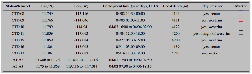
A total of seven Sea-Bird SBE9 plus conductivity–temperature–depth (CTD) measurements were taken throughout the entire water column over a period of 5 weeks from 2 April 2019 to 17 May 2019 (Table 1). Depending on the position of the eddy as obtained from altimeter data analysis, various CTD casts were conducted at the center and rim of the eddy to characterize its seawater mass properties. The CTD casts 08 (at center), 09 (western rim), 10 (western rim), and 11 (reference station) were taken within 2 d along 11.9^∘ N in the E–W direction across the nearly 4^∘ of longitude influenced by the eddy. CTD 11 was obtained outside of the eddy periphery as a reference station in order to determine the eddy impacts on the seawater properties relative to the eddy (Table 1). Subsequently, CTD casts were repeated at the reference station (CTD 11) over a 5-week period at the western rim (CTD 15), center (CTD 16), and eastern rim (CTD 17) of the eddy as it moved toward the polymetallic nodule exploration areas in the CCZ. The CTD frame was also equipped with an upward-looking and a downward-looking Nortek Aquadopp 2 MHz recording every second with 20 bins with 0.5 m blanketing. During the upcast, the CTD paused for 10 min at 50, 150, and 250 m and every 500 m below it to collect current data that were not distorted by movement of the CTD. The data quality from the upward-looking Aquadopp was poor; therefore, we only show data from the downward-looking Aquadopp.

For further investigation of the eddy effects on the seawater properties, we use the World Ocean Atlas 2018 (WOA18) for a temperature, salinity, and dissolved oxygen concentration climatology in our study. The WOA18 is a collection of objectively analyzed, quality-controlled temperature, salinity, oxygen, and other oceanographic parameters based on profile data from the World Ocean Data base with a horizontal resolution of $\mathrm{1}/{\mathrm{4}}^{\circ }$ and 102 vertical layers covering 13 years between January 2005 and December 2017 (Locarnini et al., 2018; Zweng et al., 2018; Garcia et al., 2018). The WOA18 data are available at https://www.ncei.noaa.gov/products/world-ocean-atlas (last access: 28 July 2022). Eddy-induced anomalies for each ocean parameter (T, S, and ρ) were obtained by subtracting our measurements from the long-term WOA18 climatologies for every parameter.

Table 1 Positions and characteristics of CTD and ADCP deployment across the eddy.

2.2 ADCP measurements

While the ship was underway and when being on stations, the hull-mounted acoustic Doppler current profiler (ADCP 75 kHz) almost continuously measured the upper-ocean current structure. To calculate the correct ocean currents from a moving vessel, the exact speed vector of the vessel, which is derived from the navigation and motion sensors, was subtracted from the flow fields observed by the ADCP. The vessel-mounted ADCP covered 40 bins of 16 m from 24 to 648 m water depth. Quality control analysis of the measurements shows that the ADCP recorded meaningful data for a depth range of up to 500 m. The location of transects and detailed information on positions and deployment time are shown in Fig. 2 and Table 1.

2.3 Satellite data and eddy detection process

The altimeter data used in this study to identify and track mesoscale eddies were obtained from the COPERNICUS Marine Environment Monitoring Service (CMEMS) and are freely available at http://marine.copernicus.eu (last access: 28 July 2022). The altimeter data used in our study are the near-real-time level-4 sea surface height and derived variables measured by multi-satellite altimeter observations over the global ocean with $\mathrm{1}/\mathrm{4}$^∘ spatial resolution and a daily temporal resolution from 1 January 2018 to 1 June 2019. The position of the eddy was tracked in near-real time using an EDA at the University of Bremen in Germany and subsequently communicated to the scientists on board RV Sonne to define the sampling program and locations (Fig. 3). In order to perform the most efficient CTD observations, an EDA and a simple forecasting method were simultaneously used to determine the center, shape, radius, and translation velocity on a daily basis. Among the identified long-lived eddies, the one which was anticipated to most likely pass through the location of the German exploration contract area (eastern CCZ) was selected. A previous study in this area (Purkiani et al., 2020) shows that most of the long-lived ACEs in the NETP converge to a meridional corridor between 10 and 12^∘N. In that study, an automated EDA developed by Nencioli et al. (2010) was applied and tested on the long-term sea level anomaly (SLA) data to identify and characterize the mesoscale eddies in this region. To forecast the eddy center positions, a simple prediction method based on the average eddy position within the 7 d prior to the desired day was performed as follows:

$$\begin{array}{}\text{(1)}& [X,Y{]}_t=[X,Y{]}_{t-\mathrm{1}}+T\times [\stackrel{\mathrm{‾}}{U},\stackrel{\mathrm{‾}}{V}],\end{array}$$

where X_t and Y_t are the new geographical position, X_t−1 and Y_t−1 are the old position, $\stackrel{\mathrm{‾}}{U}$ and $\stackrel{\mathrm{‾}}{V}$ are the average translation velocity of the eddy (cm s⁻¹) based on the 7 d prior to time t, and T is the time interval in seconds.

2.4 Reanalysis products

Since the 3D structure of the eddy cannot be inferred from individual CTD casts, an eddy-resolving global ocean reanalysis product was employed (Drévillion et al., 2018; Lellouche et al., 2021), with a horizontal resolution of $\mathrm{1}/\mathrm{12}$^∘ and 50 vertical layers covering the time period between January 2018 and June 2019. The T and S anomalies are calculated referenced to the climatological annual mean temperature and salinity obtained in 2018, which are interpolated to the location of CTD casts. The aim was to distinguish T^′ and S^′ induced by eddies by comparing the seawater properties in the presence of an eddy with 1 year of climatological T and S data. Seawater properties were interpolated to the position and time of the CTD casts, validated against them, and then presented in our results.

2.5 Heat and salt transport equations

Following previous studies (Dong et al., 2014; Yang et al., 2015; Lin et al., 2019), we obtained an estimate of the zonal heat and salt transport fluxes induced by eddies in this region. The composite three-dimensional structures of temperature anomalies, salinity anomalies, and swirl velocity were considered, and the zonal heat ($H_{\mathrm{f}}^x,\mathrm{W}{\mathrm{m}}^{-\mathrm{2}}$) and salt ($S_{\mathrm{f}}^x,\mathrm{kg}{\mathrm{s}}^{-\mathrm{1}}{\mathrm{m}}^{-\mathrm{2}}$) fluxes were calculated as follows

$$\begin{array}{}\text{(2)}& {\displaystyle }{H}_{\mathrm{f}}^x=\mathit{\rho }{C}_p{U}^{\prime }{T}^{\prime },\text{(3)}& {\displaystyle }{S}_{\mathrm{f}}^x=\mathrm{0.001}\mathit{\rho }{U}^{\prime }{S}^{\prime },\end{array}$$

where ρ is the density of sea water, U^′ is the zonal velocity deviation from mean long-term velocity, and $C_p=\mathrm{4187}\mathrm{J}{\mathrm{kg}}^{-\mathrm{1}}{}^{\circ }{\mathrm{C}}^{-\mathrm{1}}$ is the specific heat capacity. The factor 0.001 converts salinity to a salinity fraction (kilogram of salt per kilogram of seawater). The transports estimated above are usually zonal, since eddies in the NETP often travel westward. The meridional components can be readily obtained by replacing V^′ and the proper T^′ and S^′ in the zonal transects. As a result the heat (HT) and salt (ST) anomalies transported by an eddy can be estimated by integrating the eddy's area from the trapping depth (h_t) to the surface:

$$\begin{array}{}\text{(4)}& {\displaystyle }\mathrm{HT}=\underset{h_{\mathrm{t}}}{\overset{\mathrm{0}}{\int }}\int \mathit{\rho }{C}_p{T}^{\prime }{U}^{\prime }\mathrm{d}y\mathrm{d}z,\text{(5)}& {\displaystyle }\mathrm{ST}=\underset{h_{\mathrm{t}}}{\overset{\mathrm{0}}{\int }}\int \mathrm{0.001}\mathit{\rho }{S}^{\prime }{U}^{\prime }\mathrm{d}y\mathrm{d}z.\end{array}$$

In contrast to assuming a depth of no motion at 1200 m (e.g., He et al., 2018), heat transport and salt transport were calculated by integrating Eqs. (4) and (5) for the upper 1500 m water depth, where the sign of the temperature anomaly changes.

3 Results

3.1 Validation of reanalysis model products

We used the in situ CTD observations to validate the products of the reanalysis model at four stations. The comparison of the vertical temperature and salinity profiles of the in situ observations and the reanalysis model is shown in Fig. 1. The validation shows that the model results qualitatively match the observations at all water depths. The differences between model results and observations for temperature are shown at Fig. 1e. The temperature profiles show a bias of about ±0.8 ^∘C at near-surface depth that reduces to smaller than ±0.05 ^∘C at deep water. The reanalysis model results show a positive near-surface salinity off-set of about 0.2 psu at all stations. Since the bias is consistently reproduced by the model at all stations, the error in the calculation of the eddy-induced salinity anomaly obtained from the reanalysis model products is trivial (Fig. 1j). It is therefore concluded that the quantitative agreements between model results and in situ observations are sufficient for a model-based analysis of temperature and salt anomalies and the corresponding heat and salt transport in this region.

Figure 1 (a–d) Validation of reanalysis model results with in situ temperature observations at CTD stations of 08, 09, 10, and 11. (e) The bias between3 observations and reanalysis model results for temperature (ΔT). (f–i) Validation of reanalysis model results with in situ salinity observations at the same stations. (j) The bias between observations and reanalysis model results for salinity (ΔS). The observations and model results are shown as a solid line and squares at each station.

3.2 Eddy formation and its characteristics

Using an EDA on 24 years of altimeter data, Purkiani et al. (2020) showed that between four and six long-lived (lifetime >90 d) ACEs are generated annually in this region, mostly in the vicinity of the TT and PP gap winds. They travel distances of more than 1000 km into the open ocean through a narrow meridional corridor between 10 and 12^∘ N and reach the eastern CCZ (German contract area) with a time delay of approximately 5–6 months (Fig. 2a).

Figure 2 (a) Northeastern tropical Pacific Ocean (NETP) and orographic features of Central America. The location of Tehuantepec (TT) and Papagayo (PP) gap winds are shown as red boxes. The general trajectories of long-lived eddies in the ocean generated at TT and PP are shown as red arrows obtained from the analysis of long-lived eddies obtained from Purkiani et al. (2020). The study area and location of hydrographic survey are shown by the black box. (b) Locations of CTD stations are indicated as red boxes. Two ship transects (A1–A2 and A2–A3; black lines) were carried out to cross the eddy and investigate surface currents using the ship's ADCP. Exact positions of CTD stations and surface currents on transects are described in Table 1. The bathymetry is shown by the blue background colors.

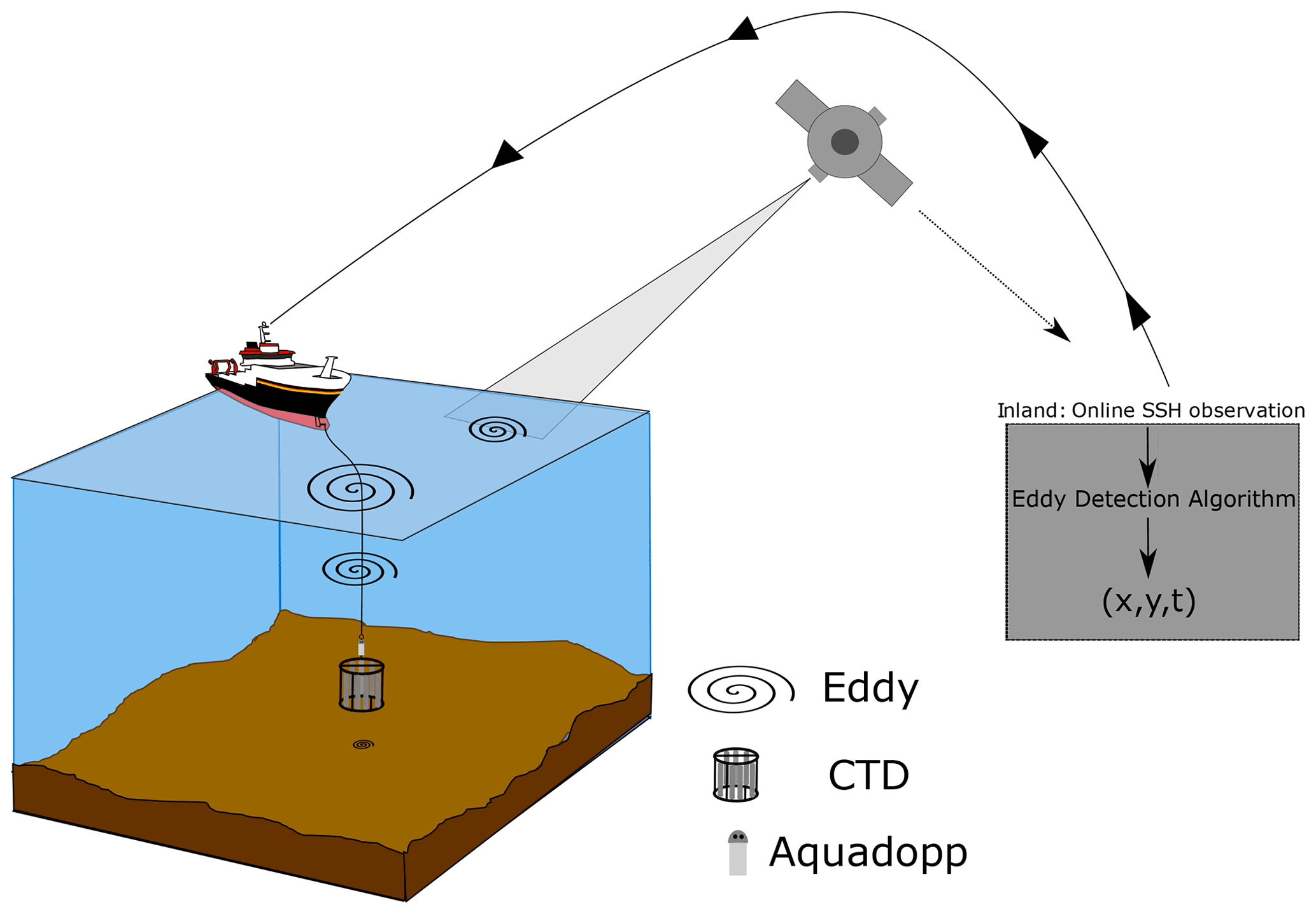
Figure 3 The concept of online communication between the research vessel in the NETP and the shore-based eddy detection group using online satellite data for determining the positions for hydrographic measurements. Figure is not to scale. Eddy, CTD, and Aquadopp are shown.

The SLA data from 1 January 2018 to 1 July 2019 were used to identify mesoscale eddies in the NETP. A total of 763 CEs and 745 ACEs with a lifetime of more than 7 d were identified, of which only two CEs and seven ACEs were characterized as long-lived eddies (lifetime > 90 d). We focused our efforts on one particular ACE that originated at TT and that crossed over the German contract area in the CCZ at the time of the SO268 expedition. The analysis of wind field data in the TT gap wind region showed a sudden development of a strong wind burst event exceeding 7 m s⁻¹ for a short period of 9 d between 7 and 16 July 2018. The statistical characteristics of the long-term wind data over a 31-year period at the isthmus of TT indicate a strong seasonal variability, with maximum values in the boreal winter (November–February) and a relative maximum in July (Romero-Centeno et al., 2003). Analysis of altimeter data shows that the secondary maximum wind intensity in the TT gulf formed a long-lived ACE in this region between 15 and 23 July 2018. The formation of a long-lived ACE in July is unusual and has not been reported in previous studies from this region. The eddy remained stationary in the gulf of TT from August to December 2018 and only separated from the coast in January 2019. The movement of the eddy center into the NETP for the next 9 months is depicted by the blue circles in Fig. 4a (time interval of 7 d). The mean diameter of the eddy is estimated at 230 km with an average translation speed of 11 cm s⁻¹ since January 2019. Our series of in situ observations to elucidate eddy impacts on seawater characteristics occurred at a distance of 2050–2400 km away from origin (between 2 April and 16 May 2019).

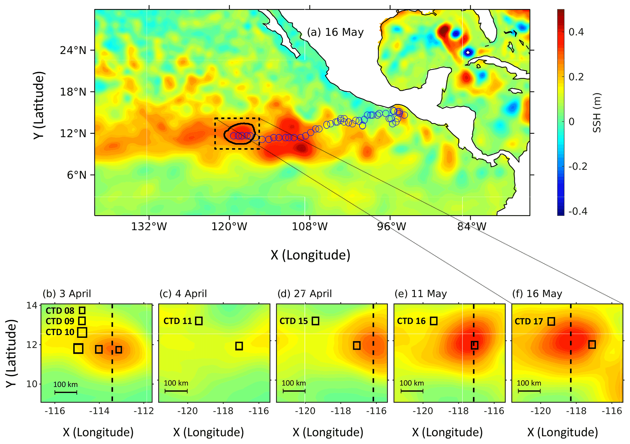
Figure 4 (a) Satellite altimeter sea surface height (SSH) data for 16 May 2019. The under-study eddy is detected using a geometry-based algorithm, and its edges are shown by the solid black lines. The weekly eddy trajectory of the ACE analyzed in this study is shown by the blue circles from 1 August 2018 to 20 May 2019. Five configurations of the eddy are shown for (b) 3 April, (c) 4 April, (d) 27 April, (e) 11 May, and (f) 16 May. The black squares show the location of CTD profiles obtained in our study. The dashed black lines show the locations of zonal transects with maximum sea surface height at which vertical profiles of seawater properties were analyzed.

3.3 Water mass properties in the NETP

The NETP is influenced by two large subtropical gyres in its upper layers: the North Equatorial Current (NEC) to the north of the eddy belt and the North Equatorial counter-current (NECC) to the south of the eddy belt. The climatological average of temperature and salinity obtained from WOA18 over an area of 1^∘ by 1^∘ centered at the position of CTD 08 is shown in Fig. 5a–b. The shaded area for T and S shows the temporal standard deviation at each depth. Four prominent water masses characterize the water column in this area: Tropical Surface Water (TSW), Equatorial Surface Water, Subtropical Surface Water, and California Current Water (Fiedler and Talley, 2006; Portela et al., 2016). Here, TSW is characterized by a sea surface temperature reaching up to 28.5 ^∘C and a sea surface salinity of about 33.7 psu. Beneath the warm and low-salinity TSW, a pronounced pycnocline caused mainly by a strong, shallow thermocline and reinforced by halocline is observed, which does not, however, contain a distinct water mass of any substantial volume (Wyrtki, 1996; Fiedler and Talley, 2006). Below the pycnocline, a water mass with S>34.6 psu and T between 10 and 14 ^∘C characterizing the Eastern North Pacific Central Water (ENPCW) is evident. Between 500 and 1000 m, the T–S diagrams (Fig. 5b) show a mixture of Antarctic Intermediate Water (AAIW; S>34.5 psu, 2–10 ^∘C) and Pacific Intermediate Water (PIW; $\mathrm{34.5}<S<\mathrm{34.9}$ psu, 4–9 ^∘C). In deep waters >2500 m, North Pacific Deep Water (1.2–2 ^∘C; S>34 psu) is present. Below 4000 m depth a water mass with temperature of about 1.2 ^∘C and salinity of 34.68–34.7 psu is attributed to Lower Circumpolar Water (LCPW), which in the eastern Pacific Ocean is characterized by high oxygen concentrations (Fiedler and Talley, 2006). The surface water layer is saturated with dissolved oxygen (>180 µmol kg⁻¹). The oxygen concentration decreases rapidly to sub-oxic concentration (<10 µmol kg⁻¹) below the oxycline at 130 m water depth. Oxygen-poor water is found below the oxycline, which extends down to 900 m depth. This oxygen minimum zone with a thickness of at least 600 m is evident in the entire NETP due to a lack of oxygen-rich deep water formation in the Pacific Ocean (Kamykowski and Zentara, 1990; Karstensen et al., 2008; Stramma et al., 2014). The T–S diagram of the no-eddy situation (CTD 11, orange line in Fig. 5b) remains in the range of the standard deviation as shown by the shaded areas in the original T–S profiles (Fig. 5a). However, the T–S diagrams of the seawater in the presence of the eddy deviates from the annual standard deviation at the sea surface and at depths between 300 and 550 m (Fig. 5a–b).

.

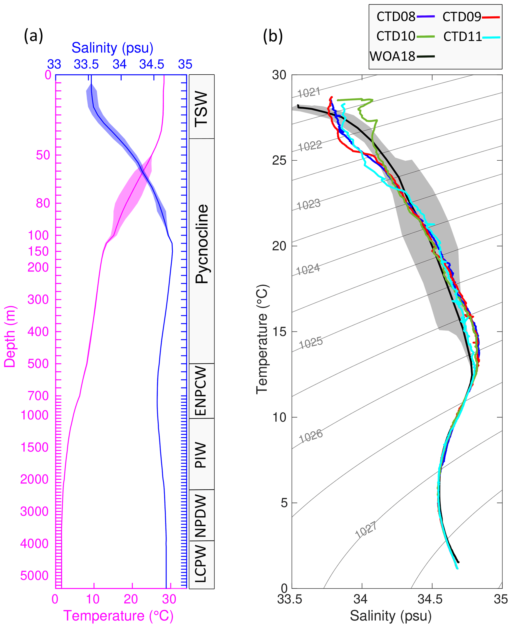
Figure 5 (a) Long-term climatology profiles of temperature and salinity obtained from WOA18 averaged over an area of 1^∘ by 1^∘ centered at the position of CTD 08 (see Table 1). Standard deviation calculated from 13-year-long time series is shown as the shaded area in pink and blue for temperature and salinity. The vertical water mass distribution is shown on the right-hand side: Tropical Surface Water (TSW), Pycnocline Layer (Pycnocline), Eastern North Pacific Central Water (ENPCW), Pacific Intermediate Water (PIW), North Pacific Deep Water (NPDW), and Lower Circumpolar Water (LCPW). (b) T–S diagram determined from WOA18 climatology data and CTD data comparing the impact of eddy on seawater properties. CTDs 08, 09, and 10 are affected by the eddy, and CTD 11 is shown as the reference station for comparison. Isopycnals are depicted as grey lines with an interval of 0.5 kg m⁻³

3.4 Temperature, salinity, and oxygen anomalies induced by the eddy

The vertical temperature (T), salinity (S), and dissolved oxygen (DO) profiles obtained from an E–W transect across the eddy center (Fig. 2b) measured within 2 d from 2 to 4 April 2019 are shown in Fig. 6a, c, e. To further illustrate eddy impacts, we have determined the anomalies of these seawater properties, which are considered a deviation from the background ocean state, by subtracting the climatology data (WOA18) at the relative location of each station from individual vertical hydrographic profiles (Fig. 6b, d, f). The eddy has significant but variable impact on the T, S, and DO profiles of the water column. In the presence of the eddy, all CTD profiles show warmer and fresher seawater in the upper 500 m (Fig. 6). The major impact of the eddy on seawater T is confined to the upper 500 m of the water column, with a maximum anomaly of +8.2 ^∘C at 92 m water depth, which is the position of the seasonal thermocline in this region. The seawater T anomalies decrease to intermediate water depth, with only a weak positive anomaly of 0.05 ^∘C at 1500 m water depth, and become negligible below that. A maximum S anomaly of −0.78 psu is located at 91 m water depth. In contrast to T, S shows no significant alteration below 500 m. However, the second (positive) and third (negative) anomalies known as the weak salinity dipoles (Nan et al., 2011) were only discernible at 150–300 and 300–700 m depth. The DO distribution is also affected by the eddy, with an increase up to 120 µmol kg⁻¹ in the subsurface layers. However, the eddy appeared to negatively affect the oxygen-poor water content below the pycnocline and increased the hypoxia at depths between 150 and the seafloor. A negative DO anomaly of −5 µmol kg⁻¹ is observed below the oxycline and remains to the deeper part of the ocean. Interestingly, the intensity of anomalies observed in T, S, and DO is larger at the center than the western rim of the eddy (compare the red and blue lines with the green and black lines in Fig. 6h, j, l). According to the criteria of Montégut et al. (2004) for the calculation of the mixed layer depth (MLD), the eddy has deepened the MLD by 10 m from 66 m in the western rim to 76 m at the center of the eddy. The ACE deepened the thickness of the thermocline layer by 15 m from 43 m at the western rim (CTD 11) to 58 m at the eddy center (CTD 08) when passing the study area. The deepening of the thermocline is in agreement with the classical impact of anticyclonic eddies on seawater characteristics derived from both local (Chen et al., 2010) and global measurements in the oceans (Gaube et al., 2019).

Figure 6 Vertical profiles of (a) temperature, (c) salinity, and (e) dissolved oxygen concentration and of anomalies in the parameters at (b), (d), and (f) respectively. The top panels show each parameter and its anomaly on an east–west transect between 2 and 4 April. The relative position of the CTD casts with respect to the eddy is shown in (a) and (g). Panels (g), (i), and (k) show vertical profiles of temperature, salinity, and dissolved oxygen in replicate CTD casts at the same position between 4 April and 16 May. Associated anomalies of temperature, salinity, and dissolved oxygen are shown in (h), (j), and (l), respectively. For a better focus on upper ocean layers, a non-equivalent vertical y axis is applied in this figure. Every anomaly is calculated with reference to the corresponding profile of WOA18.

The impact of the eddy on seawater properties was further investigated by conducting repeated CTD measurements while the eddy was approaching and passing over the location of the CTD 11 station within 5 weeks between 4 April and 16 May 2019 (Fig. 2b). A larger maximum T anomaly of 9.8 ^∘C located at 92 m water depth was observed. The maximum S anomaly of −0.78 psu in the eddy core at 92 m water depth remains as before. The DO showed higher anomalies of +137 µmol kg⁻¹ at the eddy core. In agreement with the measurements taken at CTDs 08, 09, 10, and 11, T anomalies could be distinguished down to greater depth than S anomalies. Also, the observed anomalies of all seawater properties were found to be stronger in the western and central segments of the eddy compared to the eastern segment, and the major impacts were confined to the upper 500 m of the water column. In general, the stronger influence of eddies at CTDs 15, 16, and 17 could be attributed to the different background water mass in this region. The T anomalies observed in our study are significantly larger than in most previously reported measurements, in which a warmer eddy core of between 1.5 and 5 ^∘C was registered, e.g., in the Indian Ocean (Lin et al., 2019; Yang et al., 2015), in the Pacific Ocean (Ji et al., 2018; Chaigneau et al., 2011; Stramma et al., 2014; Czeschel et al., 2018), in the SCS (Nan et al., 2017; He et al., 2018; Chen et al., 2010), and in the Arctic Ocean (Nishino et al., 2011). However, one similar anomaly induced by an extremely large ACE with a warm (+7.7 ^∘C) and fresh core (−0.8 psu) was observed in the SCS by Chu et al. (2014).

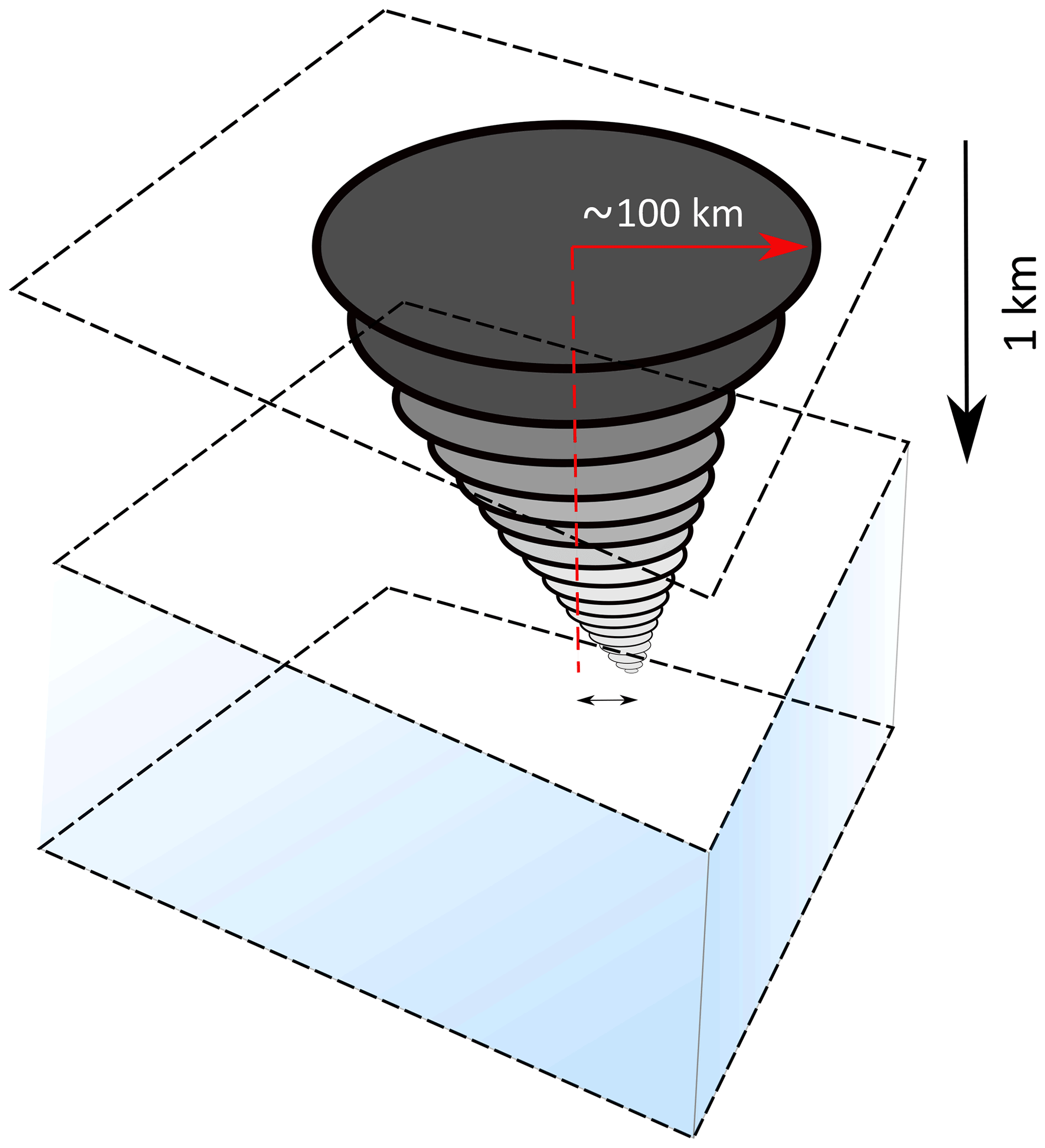
To better illustrate the seawater anomalies induced by the ACE in the water column from 2 to 4 April 2019, we show the anomaly of T, S, ρ, and DO in reference to WOA18 along the E–W transect (A2–A3, CTDs 08, 09, 10, and 11) through the eddy center (Fig. 7). In general, impacts are greatest at the center of the eddy and decrease toward the western rim of the eddy, with the least impact on seawater properties at Station 11. The T anomaly reaches a maximum of up to +8.2 ^∘C in 90 m water depth near the eddy center, whereas anomaly values of +1, +0.5, and +0.05 ^∘C extend down to 250, 350, and 1500 m water depth, respectively. This is accompanied by a decrease in the salinity of seawater by −0.78 psu in the eddy core. Following the T and S profiles, the seawater density decreases by 2.5 kg m⁻³ in the eddy core. The oxygen anomaly displays a more complex pattern, expressed most clearly at the eddy core, with a maximum positive anomaly value of 120 µmol kg⁻¹ but negative values in the sub-surface regions from 300 m down to the seafloor. The marginally negative oxygen anomalies ($\approx -\mathrm{5}$ µmol kg⁻¹) reach the seafloor at 4000 m water depth. The impact of the eddy on the fluorescence (FL) profile is mainly reflected by a deepening of the maximum fluorescence in the eddy center (1.45 mg m⁻³) of about 15 m, which, in comparison to a no-eddy situation, causes a maximum anomaly of +0.6 mg m⁻³ at the eddy core (not shown here). Except for temperature, the other parameters show a dipole-like pattern with different tendencies at the surface and the subsurface regions. This is in agreement with the findings of Nan et al. (2011) that suggested ACE in SCS indicates a dipole salinity pattern in the ocean. Moreover, a spatial lag of about 100 km between the SSH maximum (station 08) and the maximum impact of eddy-induced anomalies (station 09) is observed for all seawater parameters. The seawater anomalies resemble a bottom-up, straight conic shape for the eddy with a height of about 1500 m and a radius of 100 km at the ocean surface, and with a tilted tail in the deeper ocean (Fig. 8).

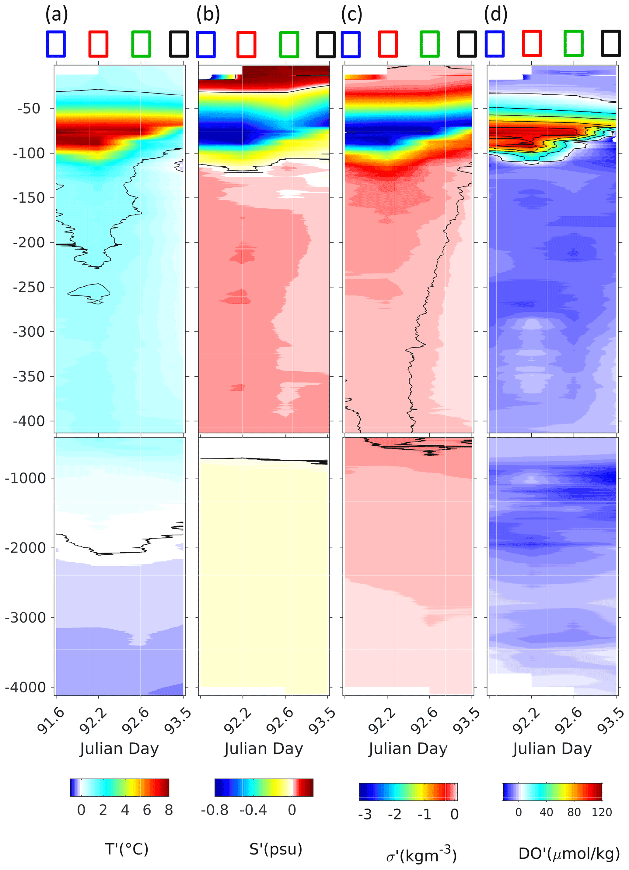
Figure 7 Vertical sections of (a) temperature anomaly, (b) salinity anomaly, (c) density anomaly, and (d) dissolved oxygen anomaly along the zonal transect of A2–A3 with respect to the WOA18 data. The color boxes at the top of each subplot (blue, red, green, and black) indicate the respective CTD stations of 08, 09, 10, and 11.

Figure 8 Schematic illustration of eddy in the water column based on reanalysis products.

3.5 Current observations across the eddy

The current velocity measured by the ship-borne ADCP during the transects A1–A2 (northeastern segment to the eddy center) and A2–A3 (eddy center to the western eddy rim) is shown in Fig. 9. The current velocity at the surface (40 m) is greater than in 200 m with maximum velocities of 40 and 20 cm s⁻¹, respectively. Moreover, current data obtained during the A1–A2 transect show a consistent clockwise rotation as is typical for an ACE. Moving along the A1–A2 transect, current velocities increased at the northeastern rim of the eddy and decreased towards the eddy center. The station carried out at CTD 08 revealed a multi-directional current at the eddy center, with a lower magnitude compared to the transect. The current velocities during the A2–A3 transect are generally lower, probably due to the incoherent SLA with lower magnitudes in the western part of the eddy. However, the northward current directions confirm the typical rotation of an ACE while it moved westward (Fig. 9). Moving from the eddy center to the western edge of the eddy along transect A2–A3, the current velocity increased to swirl velocities larger than 45 cm s⁻¹ which satisfies the eddy nonlinearity criteria ($U/c>\mathrm{3}$, where U is swirl and c is translation velocity of an eddy) defined by Chelton et al. (2011). The advective nonlinearity parameter $U/c$ is particularly useful for characterizing mesoscale eddies, since a value of $U/c>\mathrm{1}$ implies that an eddy can transport heat, salt, and potential vorticity, as well as biogeochemical properties such as nutrients and phytoplankton. Nonlinear eddies can thus have important effects on heat flux and marine ecosystem dynamics (Chaigneau et al., 2008; Hu et al., 2011; Gaube et al., 2014).

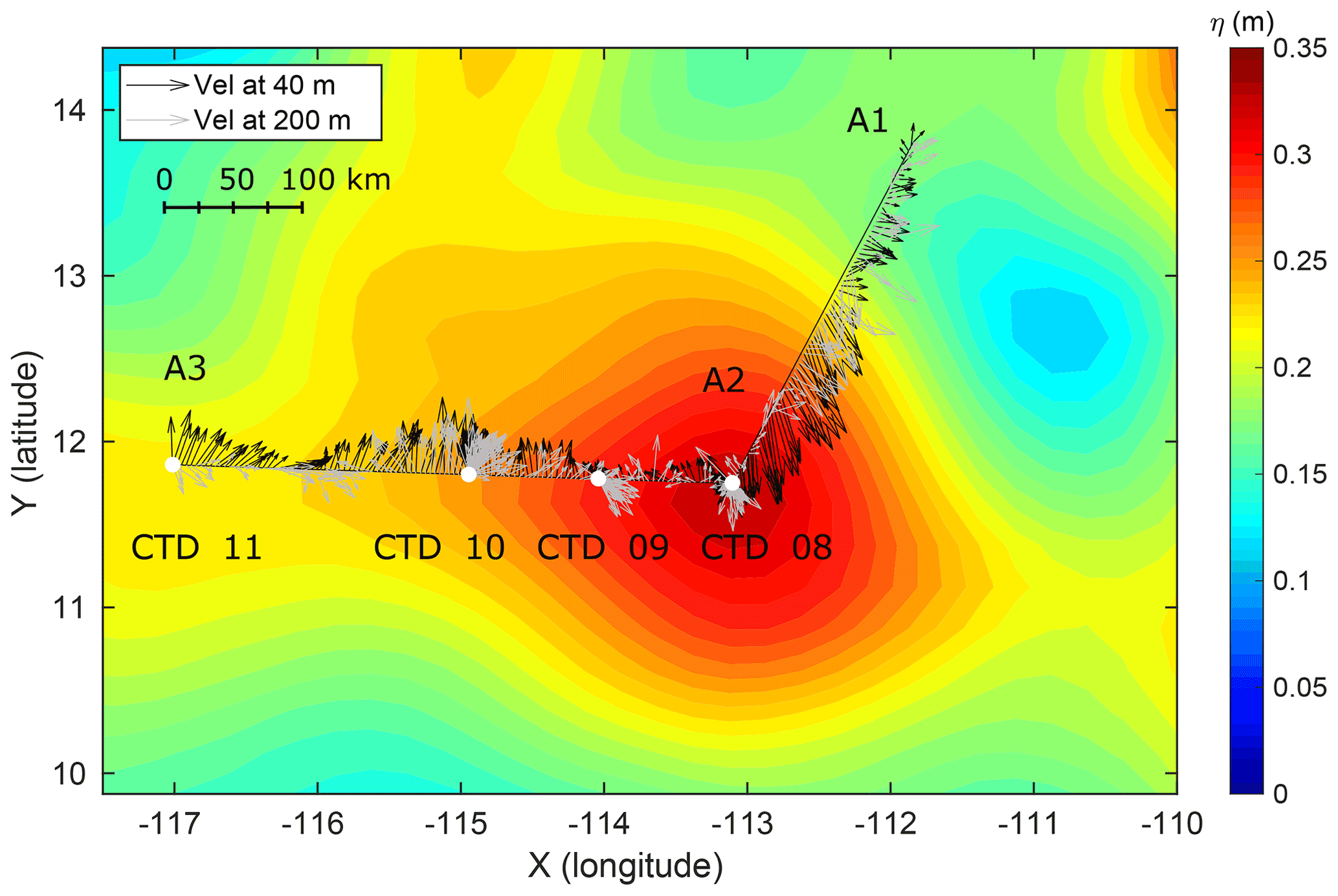
Figure 9 Current velocity at 40 and 200 m water depth as the ship was crossing the northeastern eddy segment to the eddy center (transect A1–A2) and then from the eddy center to the western eddy rim (transect A2–A3). The largest vector corresponds to a velocity of 45 cm s⁻¹. White circles show the positions and times of stations at which corresponding CTD profiles were carried out. The contour plot in the background shows SLA on 2 April 2019.

The impact of the eddy on ocean flow field is further investigated by analyzing current velocities at different depths in an E–W transect as the eddy was moving towards the German contract area. The current velocity measurements obtained from Aquadopp instruments at the CTD (15, 16, and 17) stations have been plotted at different levels of 50, 150, 250, 500, 1000, and 1500 m water depth (Fig. 10). The current velocities at the western rim of the eddy (CTD 15) generally show north-northeastward current directions in the upper layer. Below 500 m water depth, variable currents are evident (Fig. 10a). The current velocities at the center of the eddy (CTD 16) show a clear southward current direction in the upper 1000 m water depth. The current velocities at the eastern rim of the eddy (CTD 17) also show a clear southward current direction in the upper 1000 m water depth. Below that the ocean currents do not show a prevailing direction (Fig. 10c). The current velocity observations at the E–W transect portray the clockwise rotation of an ACE. Similar to the results of reanalysis products, no significant effects on ocean currents were observed at depths greater than 1000 m in our data.

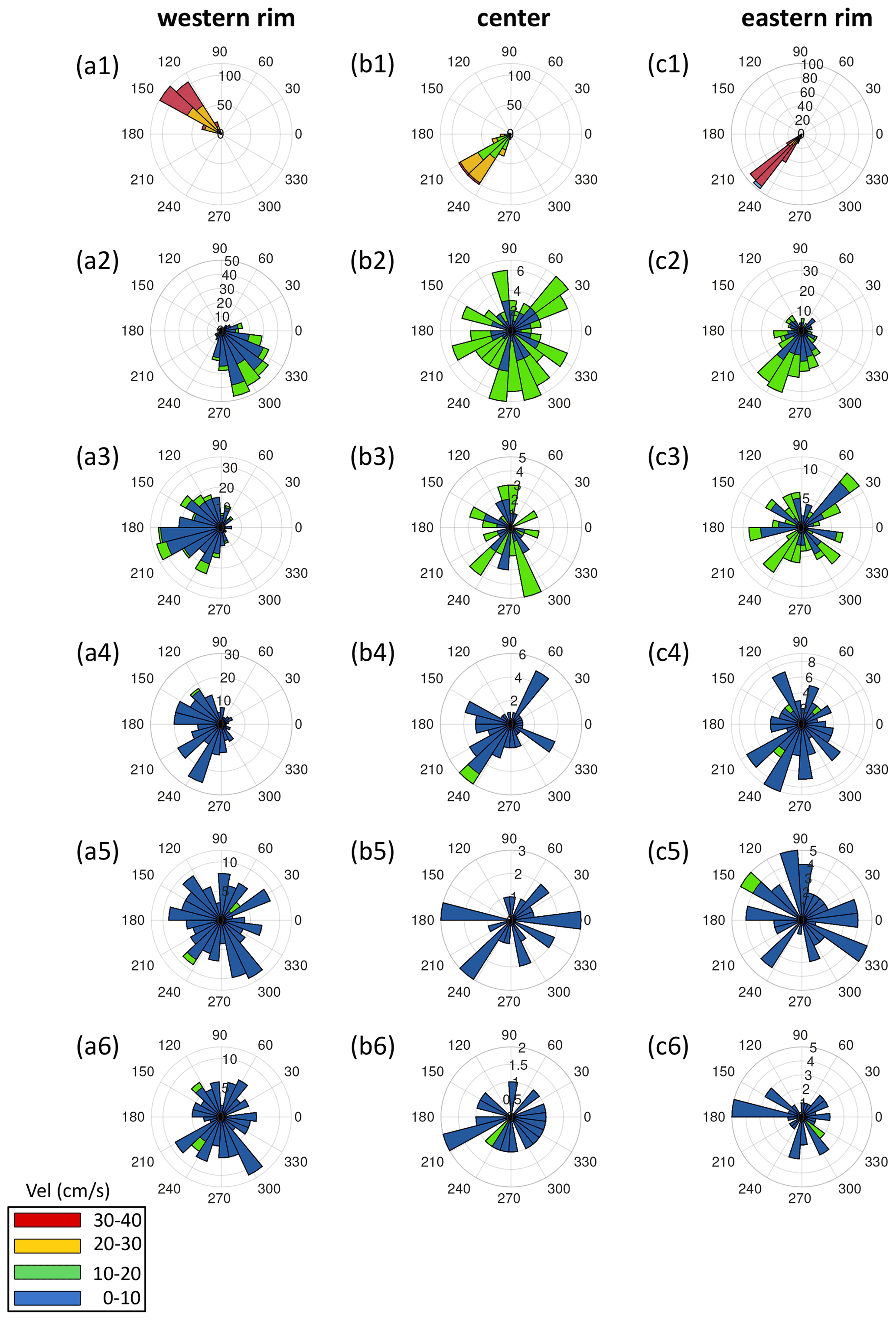
Figure 10 (a1–a6) Current velocity diagram obtained at the western rim of the eddy on 27 April. (b1–b6) Current velocity diagram obtained at the center of the eddy on 11 May. (c1–c6) Current velocity diagram obtained at the eastern rim of the eddy on 16 May. Each row from top to bottom shows the current velocity at 50, 150, 250, 500, 1000, and 1500 m water depth. Different colors correspond to the distinct current velocities indicated in the legend.

3.6 2D and 3D structure of the eddy

In the absence of detailed spatial and temporal observations, we have used reanalysis products to explore the three-dimensional structure of the eddy.

We follow the eddy while it is moving westward and show the 2D structure of vertical T, S, ρ, and velocity anomaly profiles at four different transects (see the location of transects at Fig. 4) by removing the corresponding climatological profiles averaged over 2018 from the relevant profiles at the corresponding time (Fig. 11a–h). The eddy core is located at 80–90 m and does not shoal while the eddy evolves in the ocean. The eddy footprint is more clearly distinguishable from the T anomaly than from the S anomaly and remains dominant while the eddy passes through the area. The magnitude of T^′ and S^′ reduces to values below 8 ^∘C and −0.5 psu, respectively, in the beginning of May and tends to gradually reduce by mid-May. The T anomaly decreases significantly below 300 m, although the impact of the eddy on T in intermediate water is not yet negligible. Consistent with our in situ observation, the analysis of the dynamic height of 5 ^∘C isotherms shows a vertical descent of the isotherm by about 200 m, from 910 m during the no-eddy situation to 1100 m during eddy passage. The vertical extension of the eddy as reflected by the T anomaly can be seen down to a depth of ∼1500 m. On average, the volume of trapped fluid transported by the eddy based on this cone shape is estimated to be 10×10¹² m³. This is of a similar magnitude compared to previous estimations in the South Pacific Ocean (Chaigneau et al., 2011). The center of the S anomaly observed at different depth levels coincides with that of the T anomaly, with a slightly elevated height from 30–150 m. They cannot be observed in the deeper layers. Interestingly, the positive S anomaly is observed in all profiles from the ocean surface to 35 m depth (Fig. 11e–h). The eddy core with maximum negative anomaly of about −0.5 psu is located at 85 m water depth. In agreement with the measurements, the S anomalies gradually weaken, so that the maximum of S anomalies reduced to −0.5 psu on 14 May. The vertical extents of the S anomalies are much lower than those of the T anomalies and disappear below 300 m. The limited depth of the S anomaly has been reported earlier in the SCS, where a barrier salinity layer was found to prevent anomalies from penetrating deeper into the ocean (Nan et al., 2016; He et al., 2018).

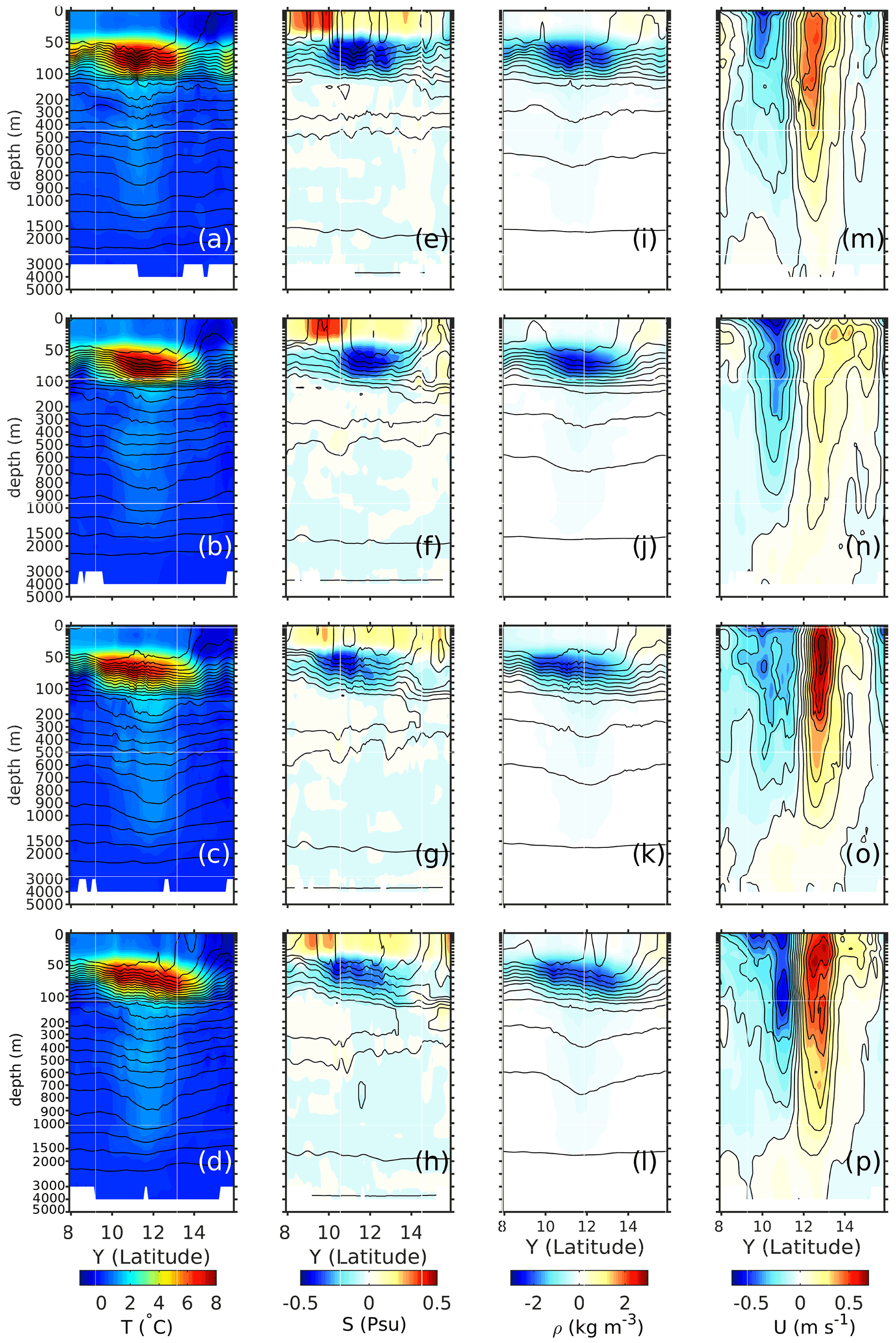
Figure 11 Vertical sections of (a to d) temperature, (e to h) salinity, (i to l) density, and (m to p) zonal velocity at 3 April, 27 April, 11 May, and 16 May 2019 (solid black lines) and their anomalies with respect to climatological mean values of 2018 (color shading). The solid lines in temperature field range between 2 and 27 ^∘C in 1 ^∘C intervals. The solid lines in salinity field range between 33 and 34.8 with 0.2 psu intervals. The solid lines in density fields range between 1021 and 1027 kg m⁻³ in 0.5 kg m⁻³ intervals, and the current field anomalies range between 0.7 and 0.7 m s⁻¹ in 0.05 m s⁻¹ velocity intervals.

Tracking the passage of the eddy through time indicates that negative density anomalies are found inside the eddy, with a maximum anomaly of −2.5 kg m⁻³ at a depth of 80 m (Fig. 11i–l). The pattern of density anomalies mainly follows the T structure, with extended impact in the deeper part driven only by temperature. In the upper layers, the zonal current velocity anomalies show a clear anticyclonic pattern with an eastward direction on the northern segment and a westward direction on the southern segment of the eddy core (Fig. 11m–p). The deeper part of the ocean (>1500 m) shows no significant anomalies, but this is likely due to the fact that the vertical resolution of reanalysis products is not good enough for this purpose.

A water column with a size of 4^∘ by 4^∘ centered in the eddy core on 3 April 2019 is considered, and the 3D structure of the eddy is plotted using ocean temperature and salinity at depths of 0, 80, 200, 300, 500, 1000, and 1500 m (Fig. 12). The seawater T anomaly isolated in the eddy shows a more symmetrical pattern than what we observe in the S field, and it is visible at 1500 m water depth describing the specific feature of an ACE (Fig. 12a). The salinity anomalies are limited to the upper 500 m water depth (Fig. 12b).

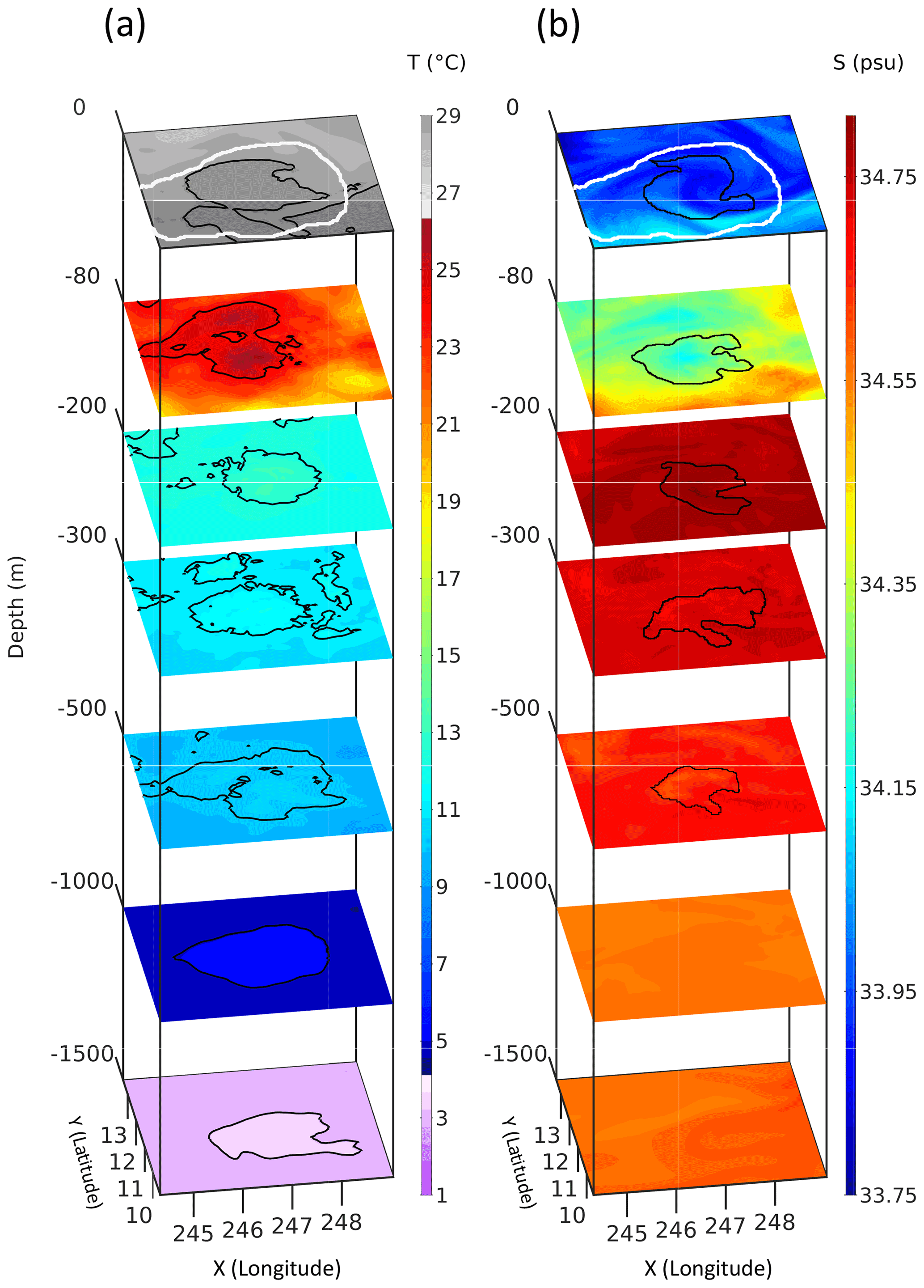
Figure 12 (a) Vertical structure of seawater temperature and (b) salinity at a box with a size of 4^∘ by 4^∘ at 80, 200, 300, 500, 1000, and 1500 m depths based on reanalysis data on 2 April 2019. Black contours show the temperature and salinity anomalies at different depths. White contour indicates the eddy perimeter derived from the sea surface height anomaly.

3.7 Eddy-induced heat and salt transport

Mesoscale eddies transport T–S anomalies owing to the advective trapping of interior water parcels, thus contributing to the regional and global heat and salt transport in the oceans (Dong et al., 2014). Generally, due to the differing CE and ACE movements and pycnocline displacement tendencies, both eddy types have negative zonal velocity (westward propagation); therefore zonal heat and salt mass transport by the two types of eddies have opposite signs and thus tend to create an equal balance. However, the greater number of long-lived ACEs in the NETP (Purkiani et al., 2020) may cause a dominant tendency toward a positive net heat flux in this region. To investigate this, we show the analysis of heat and salt transport induced by a long-lived ACE in this region.

The ACE observed in our study is highly heterogeneous in both the horizontal and vertical directions. There is a considerable zonal current asymmetry across the eddy, with stronger westward currents in the southern part of the eddy and weaker eastward currents in the northern part of the eddy. The eastward segment observed in the northern part of the eddy appears to be more vertically stretched into the deeper layers of the ocean on all occasions (see Fig. 11m–p). The rotational velocity in the eddy decreases with depth and becomes less than 0.1 m s⁻¹ below 1500 m depth. The vertical section of T^′ and S^′ shows that there are asymmetric patterns in both profiles, with tilted isotherms and isopycnals in the northern part of the eddy (see Fig. 11a–h). The combined asymmetries of T–S fields and current velocities observed in our study should demonstrate a net zonal heat (HT) and salt transport (ST) in this region.

Due to the asymmetries in seawater properties, the heat fluxes also show an asymmetric pattern with positive (eastward) and negative (westward) values in the northern and southern sections of the eddy, respectively, and with peaks of $\pm \mathrm{1.5}\times {\mathrm{10}}^{\mathrm{7}}$ W m⁻² at a depth of 90 m (Fig. 13a–d). No significant features were found below 1000 m water depth. The meridional salt fluxes of the composite eddy have different signs compared to the heat fluxes and show positive (westward) and negative (eastward) salt transport in the southern and northern parts of the eddy (Fig. 13e–h). The salt transport at 80 m depth shows an absolute peak of ±0.25 $\mathrm{kg}{\mathrm{m}}^{-\mathrm{2}}{\mathrm{s}}^{-\mathrm{1}}$. A common feature for the ACE is that the heat and salt fluxes were mainly concentrated above the thermocline (<300 m) and halocline (<150 m). Similar patterns with slightly reduced magnitude of both heat and salt transport are observed at all occasions. The meridionally integrated eddy-induced zonal HT and ST within 10–14^∘ N are strongly depth-dependent and mainly concentrated at the upper 500 m water depth (Fig. 13i–p). The HT is generally positive throughout the entire water column. It reaches its maximum of about +2 TW (10¹²W = TW) at 80 m water depth on 27 April and then drops off slightly (Fig. 13i–l). This could be due to the different background seawater temperature at the various transects. Similar to HT, significant ST transport is restricted to only the upper 1000 m in the ocean. The maximum ST reaches up to $-\mathrm{2}\times {\mathrm{10}}^{\mathrm{4}}$ $\mathrm{kg}{\mathrm{m}}^{-\mathrm{1}}{\mathrm{s}}^{-\mathrm{1}}$ at 70 m water depth (Fig. 13m–p). The vertical variation in HT and ST below 1000 m is almost negligible.

Figure 13 Vertical sections of heat flux (a–d) and salinity flux (e–h). Vertical profiles of meridionally integrated zonal heat transport (i–l) and vertical profile of meridionally integrated zonal salt transport (m–p). Each row from top to bottom shows the transects on 3 April, 27 April, 11 May, and 16 May 2019, respectively.

Integrated over the trapping depth, HT varies between +26 and 150 TW, whereas ST variation is much smaller, ranging only between −1.5 and $-\mathrm{2.8}\times {\mathrm{10}}^{\mathrm{6}}$ kg s⁻¹.

Dong et al. (2014) show that the meridionally integrated zonal HT induced by eddies in the North Pacific reaches up to 0.1 PW at 117^∘ W. Thus, the amount of HT induced by the ACE in our study is equivalent to about 1 % of the total HT at this region.

Compared to previous estimates that were carried out in the Indian Ocean (Yang et al., 2015; Lin et al., 2019), Bay of Bengal (Gonaduwage et al., 2019), and South Pacific Ocean (Chaigneau et al., 2008), we find that the zonal heat–salt transport in the NETP is more effective and one order of magnitude stronger than in the other regions. As the size and the vertical depth of eddy penetration are comparable to previous studies, the main reason for the larger HT–ST in our study is associated with the larger T and S anomalies trapped in the eddy core. The results underline the important role of eddies in the regional ocean circulation of the NETP.

4 Discussion

In the present study, the combined analysis of CTD profiles and a reanalysis dataset from the NETP provides new insights into the seawater anomalies trapped inside an ACE while it evolves in the ocean. The analysis of the CTD profiles confirms the classical picture of an anticyclonic eddy that is characterized by warmer and fresher water compared to the WOA18 data, which is in agreement with previously reported observations (Chaigneau et al., 2011; Nan et al., 2011; de Jong et al., 2014; He et al., 2018). Most studies to date indicate a T anomaly in the range of 0.65 to 5 ^∘C. The in situ observations in our study show an extremely warm eddy core with a T anomaly of about +8 ^∘C. Although such an extreme water T anomaly is not very common in the ocean, a previous study of Chu et al. (2014) from SCS reported a long-lasting ACE with a T anomaly of 7.7 ^∘C. The origin of the ACE observed in our study is in the TT Gulf, which belongs to the western Pacific warm pool region with a sea surface temperature higher than 28.5 ^∘C in spring (Wyrtki, 1996). Due to the high non-linearity of the eddy, the warm sea surface water of this region is trapped in the eddy and transported far offshore (2500 km) into the ocean. In addition, the unusually warm sea surface water could be associated with the positive phase of the ENSO cycle from late 2018 to early 2019 in this region (Cambronero-Solano et al., 2021). Moreover, the strong T anomalies may also stem from the size and intensity of the sea level anomalies. He et al. (2018) found that an increase of 10 cm in SLA from 10 to 20 cm in the SCS corresponds to an enhancement of the eddy core T anomaly of 1.5 ^∘C, from 2.5 to 4 ^∘C. Therefore, considering the relatively large SLA in our study (∼0.4 m), the unusually warm eddy core is consistent with the study of He et al. (2018) in the SCS.

Although the major eddy impact is restricted to the upper 300 m of the water column, the T anomalies are still visible at 1500 m water depth, with depressed isotherms below the eddy core (e.g., 5 ^∘C isotherm shows a vertical displacement of 200 m at a water depth of 900 m). It has been shown that the vertical extent of eddies exceeds 800 m when the eddy amplitude is greater than 20 cm (He et al., 2018). This is confirmed by the analysis of intense eddies in the SCS that extend vertically below 1000 m (Chu et al., 2014; Nan et al., 2017; Sun et al., 2018). Additionally, Zhang et al. (2016) show that a deep-penetrating eddy can reach to 2000 m with a notably strong tilting of the eddy axis up to 100 km from the surface to the bottom. The tilted eddy axis structure found in their study provides a good explanation for the previously observed 2–4-week time lag between surface eddies and their effects on near-bottom current intensification and alteration of predominant current direction in the German exploration contract area in the eastern CCZ (Aleynik et al., 2017; Purkiani et al., 2020). Interestingly, the comparison of the vertical extent of the eddy core in the same NETP area during different events in April 2013 (Aleynik et al., 2017) and April 2015 (Purkiani et al., 2020) in the same region with the current study shows that despite the profound impacts of the former events, the effects of the eddy recorded in April 2019 do not reach down to the seafloor. This could be associated with the larger SLA observed in 2013 (∼0.58 m) and 2015 (∼0.51 m) compared to the lower SLA in 2019 (∼0.4) in this region.

The core of maximum T and S anomalies was centered at water depth of 80 and 65 m, respectively, which is comparable to the depth of the eddy core observed from ARGO profiles in the SCS (Chu et al., 2014; He et al., 2018). However, it is relatively shallow compared to previously reported eddy core depths of 300 and 500 m in the northwestern and southeastern Pacific Ocean (Chaigneau et al., 2011; Nan et al., 2017).

Finally, by analyzing available global sediment trap data previously published by Lutz et al. (2007), a significant spatial distribution of particulate organic carbon (POC) fluxes to the deep ocean and sedimentation rates in the NETP were reconstructed (Vanreusel et al., 2016; Volz et al., 2018). The spatial distribution of POC flux shows a lower flux of 1.3 $\mathrm{mg}{\mathrm{C}}_{\mathrm{org}}{\mathrm{m}}^{-\mathrm{2}}{\mathrm{d}}^{-\mathrm{1}}$ in low latitudes between 6 and 10^∘N. A little further to the north in the region between 10 and 13^∘ N, higher POC fluxes ranging between 1.6 and 1.8 $\mathrm{mg}{\mathrm{C}}_{\mathrm{org}}{\mathrm{m}}^{-\mathrm{2}}{\mathrm{d}}^{-\mathrm{1}}$ were observed. Interestingly, the region of the deep sea characterized by higher POC fluxes closely corresponds to the region with a higher frequency of mesoscale eddy occurrence at the sea surface (Purkiani et al., 2020). Indeed, the temporal variation in vertical fluxes of biogenic, lithogenic, and POC fluxes has been attributed to mesoscale eddy activity in the past (Buesseler et al., 2008; O’Brien et al., 2013).

5 Summary and conclusion

On the basis of altimetry data and in situ hydrographic observations, the evolution and impact of a long-lived ACE on the seawater characteristics of the NETP were investigated during a research campaign that took place in the framework of the MiningImpact project to study the environmental impact and risks of deep-sea mining. The ACE originated in the Mexican Tehuantepec gap wind region during a strong wind event in summer 2018. Using an EDA, the eddy was successfully detected 9 months later at a distance of between 2050 and 2400 km off the Central American coast. This confirms that real-time altimeter data can be employed to detect eddies and precisely predict their path in the ocean. The particular ACE investigated here was characterized by a temperature anomaly of +8 ^∘C, a salinity anomaly of −0.75 psu, a dissolved oxygen anomaly of +160 µmol kg⁻¹, and a fluorescence anomaly of +0.8 mg m⁻³. The mixed-layer depth in the ACE deepened by 29 m and thickened by approx. 10 m. The major eddy impact was confined to the upper 500 m of the water column, with the effect on seawater temperature being evident only until a water depth of 1500 m. The eddy had no impact on the deeper part of the ocean. The meridional and depth-integrated zonal heat and salt transports induced by this mesoscale eddy reached 85±60 TW and $-\mathrm{2.1}\pm \mathrm{0.7}\times {\mathrm{10}}^{\mathrm{6}}$ kg s⁻¹, respectively. This is comparable to 1 % of the meridionally integrated zonal heat transport at the north Pacific Ocean. The increased number of mesoscale eddies during ENSO (Palacios and Bograd, 2005) may cause an imbalance in the north Pacific heat and salt budgets. The results of this study will be useful for the deep-sea biological and biogeochemical community to investigate the connections between mesoscale eddies and deep-sea ecosystems. A combined oceanographic and biogeochemical numerical simulation is recommended to study the potential role of mesoscale eddies in deep-sea fertilizing and the growth rate of manganese nodules in the NETP. Whereas some strong mesoscale eddies passing over the area targeted for deep-sea mining change the near-bottom current regime at depths >4000 m and potentially may affect the deep seafloor and its ecosystems (Aleynik et al., 2017; Purkiani et al., 2020), weaker mesoscale eddies may only affect the properties of seawater in the upper ocean layers without affecting the hydrodynamics of the seafloor. We suggest that the depth to which the eddies affect deeper water layers is related to the height of the sea level anomalies observed at the surface. The potential role of eddy influence on the seafloor and its consequential effect on the altered dispersion of mining-related sediment plumes must be taken into consideration during impact assessments of future mining operations. Furthermore, we have shown that mesoscale eddies change the upper water column hydrographic and dynamic characteristics for several days to weeks as they pass over a particular location in the CCZ. Although the development and testing of nodule mining technology is still in its infancy, most envisaged mining operations involve the discharge of ballast waters, sediments, and nodule debris from the surface production platform into intermediate waters below the oxygen minimum zone, producing a discharge plume there. Eddies passing through the water column might change the background temperature and salinity (density) conditions as well as current speeds and directions at such discharge points. This must also be taken into consideration during future mining assessments and plume modeling activities.