Estimating the Absolute Salinity of Chinese offshore waters using nutrients and inorganic carbon data

In June 2009, the Intergovernmental Oceanographic Commission of UNESCO released The international thermodynamic equation of seawater – 2010 (TEOS-10 for short; IOC et al., 2010) to define, describe and calculate the thermodynamic properties of seawater. Compared to the Equation of State-1980 (EOS-80 for short), the most obvious change with TEOS-10 is the use of Absolute Salinity as salinity argument, replacing the Practical Salinity used in the oceanographic community for 30 years. Due to the lack of observational data, the applicability of the potentially increased accuracy in Absolute Salinity algorithms for coastal and semi-enclosed seas is not very clear to date. Here, we discuss the magnitude, distribution characteristics, and formation mechanism of Absolute Salinity and Absolute Salinity Anomaly in Chinese shelf waters, based on the Marine Integrated Investigation and Evaluation Project of the China Sea and other relevant data. The Absolute Salinity S_A ranges from 0.1 to 34.66 g kg⁻¹. Instead of silicate, the main composition anomaly in the open sea, CaCO₃ originating from terrestrial input and re-dissolution of shelf sediment is most likely the main composition anomaly relative to SSW and the primary contributor to the Absolute Salinity Anomaly δS_A. Finally, relevant suggestions are proposed for the accurate measurement and expression of Absolute Salinity of the China offshore waters.

1 Introduction

Absolute Salinity, which is traditionally defined as the mass fraction of dissolved material in seawater, replaces Practical Salinity as the salinity argument in the TEOS-10 (IOC et al., 2010) seawater standard for the thermodynamic properties of seawater. This is because these thermodynamic properties are directly influenced by the mass of dissolved constituents, whereas Practical Salinity depends only on their conductivity. Since the relative amounts of different constituents change from place to place and from time to time, accounting for the biases that are introduced by these changes may be important. However, appropriate methods for frequent and regular measurements of the dissolved content directly in ocean studies are still a topic of research.

At present, the TEOS-10 Absolute Salinity of a seawater sample is obtained by adding the Absolute Salinity Anomaly δS_A to Reference Salinity S_R, in which S_R is the mass fraction of dissolved material in a stoichiometric composition model (the Reference Composition or RC) of seawater, defined by Millero (2008), for which the reference material known as International Association for the Physical Sciences of the Ocean (IAPSO) Standard Seawater (SSW for short), is a good approximation and of the same conductivity as that of the sample. δS_A is the mass fraction change caused by composition variations relative to RC. Three algorithms for calculating Absolute Salinity in the open ocean are provided in TEOS-10. The two that avoid a direct measurement either make assumptions about the dominant biogeochemical processes in the ocean that affect the Absolute Salinity Anomaly or rely on empirically determined correlations.

However, the applicability and accuracy of the TEOS-10 algorithms are still not very clear for estuaries and semi-enclosed oceanic basins where the relative compositions of the seawater may be different from that of the open ocean. Although there have only been very few direct measurements of conductivity and density in such areas (Millero, 1984; Feistel et al., 2010a), Pawlowicz (2015) used chemical-composition–conductivity–density modeling and climatological data to estimate the Absolute Salinity Anomaly near many rivers around the world, finding values of up to 1 order of magnitude higher than those extrapolated from the open ocean.

The coastal areas of China comprise one of the widest shallow seas in the world, with a large north–south span, numerous estuaries and bays, and a large amount of freshwater input from rivers. The relative composition of this coastal seawater may not only differ from that of the open ocean but also vary from place to place. However, the influence of relative composition variation on the Absolute Salinity in this area has never been systematically studied, although salinity measurement has played an important role in Chinese national ocean survey projects since 1957 (CSTPRC, 1964) and for metrological purposes a Chinese primary seawater standard has been developed (Li et al., 2016). Moreover, in any efforts to detect salinity variations associated with climate change variability in the Bohai and northern Yellow seas (Wu et al., 2004a, b; Xu, 2007; Lv, 2008; Song, 2009), Practical Salinity S_P is still used as the simplicity of Absolute Salinity, and its change caused by the relative composition variation is ignored. That will raise obvious problems in the correct presentation of time series and/or transects that begin near the coast and end well offshore (Wright et al., 2011).

Therefore, in this paper we first clarify the definition, status, and application of TEOS-10 Absolute Salinity. Second, based on the measured data and related research results, we estimate the magnitude, temporal and spatial distribution characteristics, and formation mechanisms giving rise to Absolute Salinity Anomalies in Chinese coastal seawaters. Finally, based on the above results, we put forward relevant suggestions and future research directions for the accurate measurement and expression of Absolute Salinity of Chinese offshore seawaters.

2 Methods and data

2.1 Calculation of Absolute Salinity

The TEOS-10 Solution Absolute Salinity of seawater is essentially based on adding up the mass of solute in a seawater sample:

$$\begin{array}{}\text{(1)}& S_{\mathrm{A}}^{\text{soln}}=\sum _{i=\mathrm{1}}^{N_{\mathrm{c}}}{M}_i{c}_i,\end{array}$$

where c_i is the molar concentration of component i in seawater kg⁻¹, M_i is the molar mass of the component, and N_c is the number of species of component in seawater. However, it is impractical to carry out a full chemical analysis for the seawater to get the $S_{\mathrm{A}}^{\text{soln}}$ regularly. The primary and most demanding purpose of oceanographic salinity measurements is the calculation of seawater density to estimate significant ocean currents driven by sometimes tiny horizontal pressure gradients. In TEOS-10, Absolute Salinity is instead defined so that the density of seawater can be accurately calculated by the following equation:

$$\begin{array}{}\text{(2)}& \mathit{\rho }=f_{\text{TEOS-10}}(S_{\mathrm{A}},t,p),\end{array}$$

where f_TEOS-10 is a specified function. Therefore, S_A is also called a Density Salinity.

Unfortunately, although for many purposes we can treat S_A and $S_{\mathrm{A}}^{\text{soln}}$ interchangeably, at highest precisions $S_{\mathrm{A}}\ne S_{\mathrm{A}}^{\text{soln}}$ due to small changes in the relative composition of sea salt. In order to get S_A at this highest precision, Millero (2008) first defines a stoichiometric composition model (the Reference Composition or RC), based on a reference material (IAPSO Standard Seawater), and specifies an algorithm to determine a consistent estimate of the mass fraction of dissolved material in a sample of arbitrary salinity with the RC. This estimate is based on the widely used Practical Salinity S_P (UNESCO, 1981):

$$\begin{array}{}\text{(3)}& S_{\mathrm{R}}=u_{\text{PS}}\cdot S_{\mathrm{P}},\mathrm{2}<S_{\mathrm{P}}<\mathrm{42}.\end{array}$$

In Eq. (3), the factor u_PS between the Reference Salinity of Standard Seawater and the Practical Salinity is (35.16504/35) g kg⁻¹ and is not equal to 1 mainly because an evaporative technique used by Sørensen in 1900 (Forch et al., 1902) led to the loss of some volatile components of dissolved material.

General seawater can be regarded as the mixture of Standard Seawater concentrated/diluted with pure water and a small amount of other components. The calculation formula of Absolute Salinity from Reference Salinity requires the addition of a correction, the Absolute Salinity Anomaly δS_A:

$$\begin{array}{}\text{(4)}& S_{\mathrm{A}}=S_{\mathrm{R}}+\mathit{\delta }{S}_{\mathrm{A}}.\end{array}$$

At present there are three methods for determining the Absolute Salinity Anomaly δS_A. First, it can be obtained by comparisons with direct density measurements performed in the laboratory (Millero et al., 2008; Wright et al., 2011). According to the density difference $\mathit{\rho }={\mathit{\rho }}^{\text{lab}}-\mathit{\rho }(S_{\mathrm{R}},\mathrm{25}{}^{\circ }\mathrm{C},\mathrm{0}\mathrm{dbar})$ and the haline contraction coefficient, which is 0.7519 for SSW, δS_A is determined by

$$\begin{array}{}\text{(5)}& {\left.{\displaystyle \frac{\partial \mathit{\rho }}{\partial S_{\mathrm{A}}}}\right|}_{t=\mathrm{25}{}^{\circ }\mathrm{C},p=\mathrm{0}\mathrm{dbar}}\approx \mathrm{0.7519}\mathrm{kg}{\mathrm{m}}^{-\mathrm{3}}(\mathrm{g}{\mathrm{kg}}^{-\mathrm{1}}{)}^{-\mathrm{1}}.\end{array}$$

This procedure is useful for laboratory studies or in situations where ocean water can be obtained from sampling bottles retrieved from certain depths for subsequent laboratory measurements of density.

Second, it can be estimated using a correlation equation whether chemical measurements of the most variable seawater constituents in the open ocean (carbonate system and macro-nutrients) are also available (Pawlowicz et al., 2011; IOC et al., 2010).

$$\begin{array}{}\text{(6)}& \begin{array}{rl}& \mathit{\delta }{S}_{\mathrm{A}}^{\text{dens}}/\left(\mathrm{mg}{\mathrm{kg}}^{-\mathrm{1}}\right)=\mathrm{55.6}\times \mathrm{\Delta }\left[\text{NTA}\right]+\mathrm{4.7}\\ & \times \mathrm{\Delta }\left[\text{NDIC}\right]+\mathrm{38.9}\times \left[{\mathrm{NO}}_{\mathrm{3}}^{-}\right]+\mathrm{50.7}\times \left[{\mathrm{S}}_i(\mathrm{OH}{)}_{\mathrm{4}}\right]\end{array}\end{array}$$

The units of each component on the right are all millimole per kilogram, $\mathrm{\Delta }\left[\text{NTA}\right]=\text{TA}-\mathrm{2.3}\times S_{\mathrm{P}}/\mathrm{35}$ is the standardized change in Total Alkalinity (TA), and $\mathrm{\Delta }\left[\text{NDIC}\right]=\text{DIC}-\mathrm{2.08}\times S_{\mathrm{P}}/\mathrm{35}$ is the standardized change in total Dissolved Inorganic Carbon (DIC). Note that the coefficients of this model are calculated using a numerical model for chemical interactions (Pawlowicz, 2008, 2010; Pawlowicz et al., 2011), which performed well against lab studies and were shown to have reasonable accuracy for seawater samples by Wooseley et al. (2014). An important aspect of this modeling is that, in order to maintain a charge balance in the dissolved constituents, it was assumed that calcium concentrations also changed according to

$$\begin{array}{}\text{(7)}& \mathrm{\Delta }\left[\text{NTA}\right]=\mathrm{2}\mathrm{\Delta }\mathrm{N}\left[{\mathrm{Ca}}^{\mathrm{2}+}\right]-\mathrm{\Delta }\left[{\mathrm{NO}}_{\mathrm{3}}^{-}\right],\end{array}$$

in which $\mathrm{\Delta }\mathrm{N}\left[{\mathrm{Ca}}^{\mathrm{2}+}\right]={\mathrm{Ca}}^{\mathrm{2}+}-\mathrm{10656.6}\cdot S_{\mathrm{P}}/\mathrm{35}/\left(\mathrm{\mu }\mathrm{mol}{\mathrm{kg}}^{-\mathrm{1}}\right)$ and Ca²⁺ and S_P are the measured value of Ca²⁺ and Practical Salinity of seawater, respectively. Calcium was chosen to balance charge since it is (a) not usually measured but (b) it is known to vary in its relative composition by a few percent in the open ocean. However, the accuracy of this relationship is not known.

Third, Absolute Salinity Anomaly δS_A can be found from a global δS_A climatology created by McDougall et al. (2012). Due to the lack of seawater component data, McDougall et al. (2012) carried out regression calculation on the Practical Salinity, density, and silicate concentration data of 811 seawater samples worldwide and found that δS_A can be directly related to S_i(OH)₄:

$$\begin{array}{}\text{(8)}& \begin{array}{rl}& \mathit{\delta }{S}_{\mathrm{A}}/\left(\mathrm{g}{\mathrm{kg}}^{-\mathrm{1}}\right)=\left(S_{\mathrm{A}}-S_{\mathrm{R}}\right)/\left(\mathrm{g}{\mathrm{kg}}^{-\mathrm{1}}\right)\\ & =\mathrm{98.24}\left({\mathrm{S}}_i(\mathrm{OH}{)}_{\mathrm{4}}/\left(\mathrm{mol}{\mathrm{kg}}^{-\mathrm{1}}\right)\right),\end{array}\end{array}$$

although for further work the numerical coefficient was tuned for specific ocean basins. Taking the effects of evaporation and rainfall on ocean salinity into consideration, Eq. (8) can be simplified as

$$\begin{array}{}\text{(9)}& \mathit{\delta }{S}_{\mathrm{A}}=R^{\mathit{\delta }}{S}_{\mathrm{R}}\text{(except the Baltic Sea)},\end{array}$$

in which $R^{\mathit{\delta }}=\mathit{\delta }{S}_{\mathrm{A}}^{\text{atlas}}/S_{\mathrm{R}}^{\text{atlas}}$; both the $S_{\mathrm{R}}^{\text{atlas}}$ and $\mathit{\delta }{S}_{\mathrm{A}}^{\text{atlas}}$ are from the Gouretski and Koltermann (2004) hydrographic atlas.

$$\begin{array}{}\text{(10)}& S_{\mathrm{A}}=u_{\text{PS}}{S}_{\mathrm{P}}\left(\mathrm{1}+R^{\mathit{\delta }}\right)={\displaystyle \frac{\mathrm{35.16504}/\left(\mathrm{g}{\mathrm{kg}}^{-\mathrm{1}}\right)}{\mathrm{35}}}{S}_{\mathrm{P}}\left(\mathrm{1}+R^{\mathit{\delta }}\right)\end{array}$$

Equation (10) is adopted in the official Gibbs SeaWater Oceanographic Toolbox (available from http://www.teos-10.org, last access: 8 June 2021, McDougall and Barker, 2011) to calculate that δS_A with uncertainty in the ocean is less than 0.0047 g kg⁻¹. For the semi-enclosed Baltic Sea, Feistel et al. (2010a) have fitted an empirical formula for calculating δS_A, which is mainly due to rivers bringing material of anomalous composition into the Baltic Sea, and this formula has also been incorporated into the Gibbs SeaWater (GSW for short) algorithm library.

In the work described here we compare the latter two methods.

2.2 Observation data

The near-synchronous oceanographic and ocean chemical data used here are from 1480 stations covering Chinese offshore waters that were set up for the Marine Integrated Investigation and Evaluation Project of the China Sea conducted by the State Oceanic Administration of China (Xiong, 2012; Ji, 2016), as shown in Fig. 1. At these sites, surface, 10 m, 30 m and bottom values for nutrients, as well as TA and pH, are available for the four seasons of spring (April–June), summer (July–September), autumn (October–December), and winter (January–March) of 2006 to 2007. Since in situ observation of DIC is missing in this project, it is derived from pH and TA data using the CO2SYS software released by the Department of Ecology of Washington State, USA, based on the carbonate equilibrium (Lewis and Wallace, 1998).

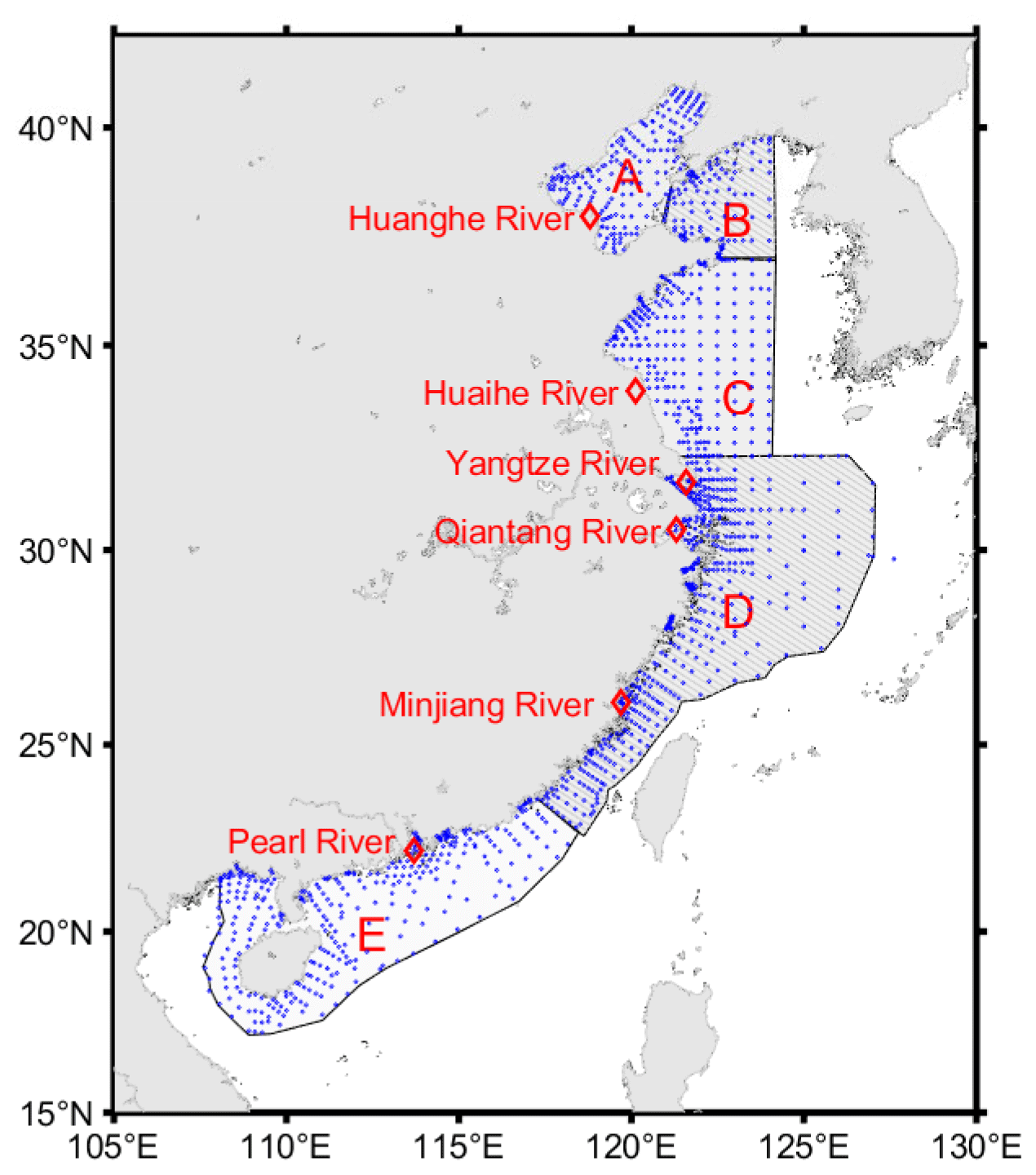
Figure 1 The geographical distribution map of sampling stations. The blue dots are the observation stations of the Marine Integrated Investigation and Evaluation Project of the China Sea. “A” is the Bohai Sea, “B” is the northern Yellow Sea, “C” is the southern Yellow Sea, “D” is the East China Sea, and “E” is the South China Sea.

3 Results

3.1 Reference Salinity S_R of the China offshore seawater

The first step in determining Absolute Salinity is to estimate the Reference Salinity based on the Practical Salinity. Because the standard PSS-78 algorithm for Practical Salinity is only valid in the range $\mathrm{2}<S_{\mathrm{P}}<\mathrm{42}$, values for samples in the mouth of the Yangtze River, Qiantang River, and Pearl River (labeled in Fig. 1) whose S_P values less than 2 are recalculated with a modified form of the Hill et al. (1986) formula based on the in situ conductivity, temperature, and pressure. Then Eq. (3) is used to get S_R.

Based on our observations (Fig. 1), the Reference Salinity S_R of Chinese offshore seawater diluted by low-salinity river runoff ranges from 0.01 to 34.66 g kg⁻¹. The extreme minimum S_R of 0.01 g kg⁻¹ appears in the south branch of Yangtze River in the summer of 2006, and the maximum of 34.66 g kg⁻¹ appears in the path of the Kuroshio Current (Fig. 2). Low salinities are also seen in the Pearl River estuary and to a lesser degree in shallow areas of the southern Yellow Sea, as well as near a few other river mouths.

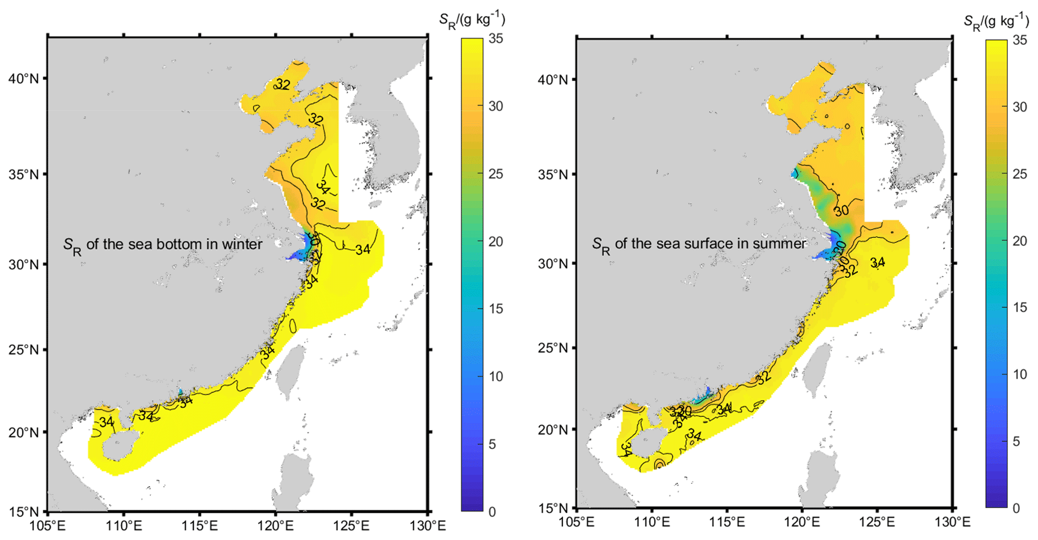
Figure 2 S_R isoclines of China offshore seawater.

3.2 Absolute Salinity Anomaly δS_A of Chinese offshore waters

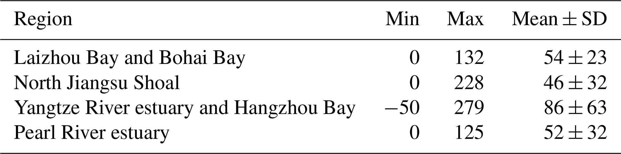
Using Eq. (6), the estimated δS_A of Chinese offshore waters ranges from −0.05 to 0.28 g kg⁻¹ (Fig. 3). The largest Absolute Salinity Anomalies are 1 order higher than those of the open ocean. As much as 90 % of the calculated δS_A arises from the Δ[NTA] term in Eq. (6), so that areas with high δS_A also have high Δ[NTA] (Fig. 4). The largest δS_A values appear in the Yangtze River estuary, Hangzhou Bay, Laizhou Bay, Bohai Bay, North Jiangsu Shoal, and the Pearl River estuary. Hangzhou Bay, which is adjacent to the Yangtze River estuary, has continuously transported water from the Yangtze River estuary due to its current and tidal characteristics (Yuan, 2009) and has almost the same water composition as the Yangtze River estuary. Thus, in this paper, the waters in the Yangtze River estuary and Hangzhou Bay are analyzed as a single water mass. The δS_A values in the above coastal regions, which are often in excess of 0.05 g kg⁻¹, are given in Table 1.

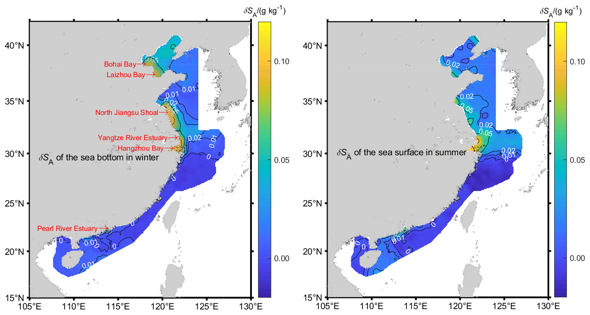
Figure 3 δS_A isoclines of Chinese offshore seawater. Hatched areas in the left figure represent the areas where δS_A is more than 0.05 g kg⁻¹.

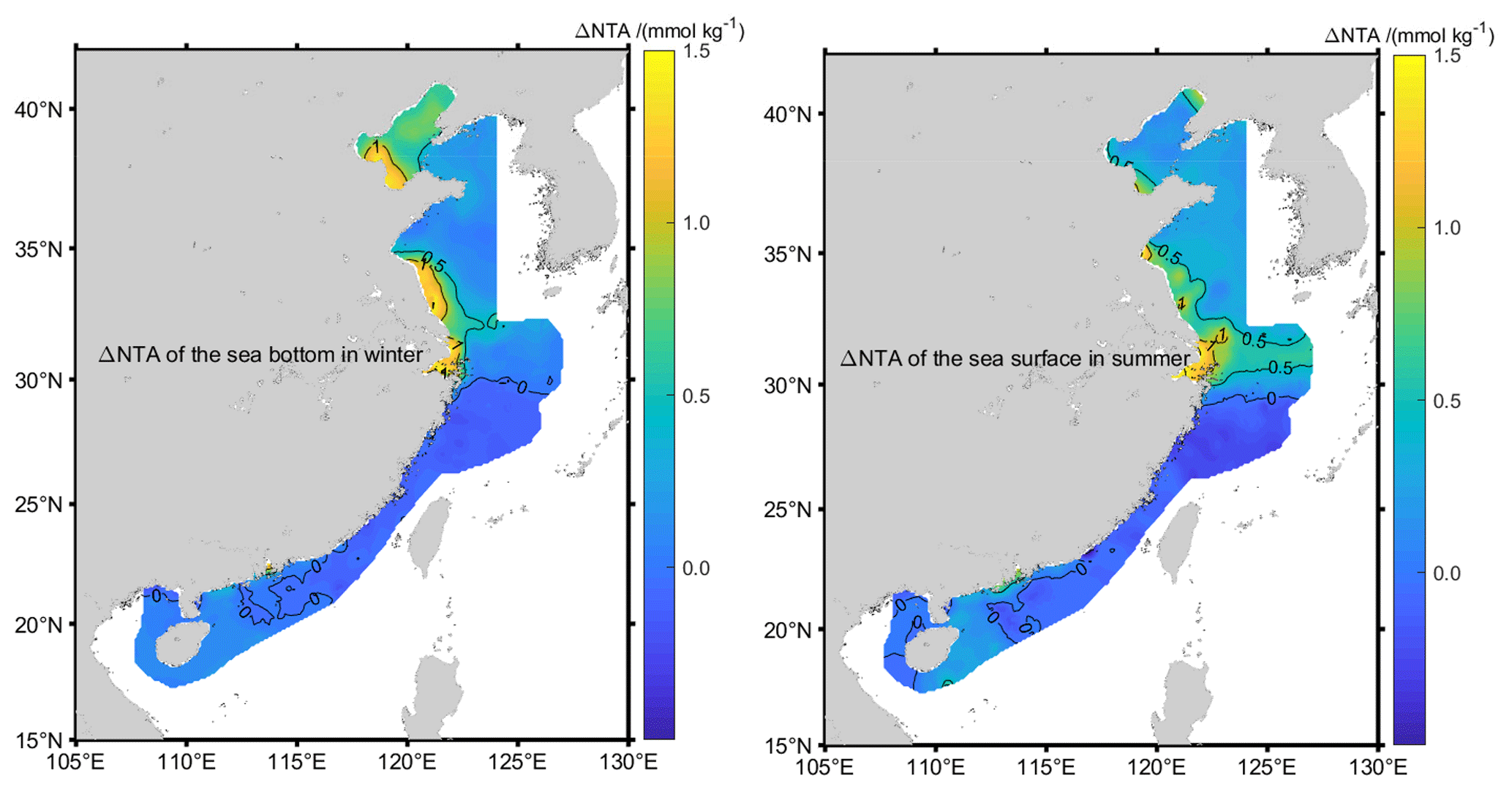
Figure 4 Δ[NTA] isoclines of China offshore seawater.

Table 1 δS_A in different coastal regions hatched in Fig. 3. Units are milligrams per kilogram.

The maximum δS_A of 0.28 g kg⁻¹ appears at the sea surface of the Yangtze River estuary and in Hangzhou Bay in summer. As China's largest runoff into the sea, the Yangtze River is rich in nutrients from land. At its entrance to the sea, the silicate concentration exceeds 100 µmol kg⁻¹, Δ[NTA] is larger than 1 mmol kg⁻¹, and the δS_A is greater than 0.1 g kg⁻¹ all year round, but these nutrient concentrations decrease rapidly away from the entrance. Δ[NTA] is the primary contributor to δS_A. The surface coverage of the 0.05 g kg⁻¹ isocline varies with seasons and depths and reaches a maximum in summer but with little variation in other seasons. In this region, 54 % and 26 % of negative δS_A appear in spring and winter, respectively, which also mainly arises from Δ[NTA].

In the northern North Jiangsu Shoal, the maximum δS_A of 0.23 g kg⁻¹ appears in the bottom layer in winter. Centered at 33.4^∘ N and 121^∘ E, many points have a δS_A greater than 0.05 g kg⁻¹ all year round, which gradually decreases from the coast to the offshore. The δS_A of the bottom layer is higher than that of the surface layer in a dry season (spring and winter) but smaller in a flood (summer and autumn) season, in which more terrestrial input is brought by Huai River system.

The largest δS_A of 0.20 g kg⁻¹ in the Bohai Sea appears at the bottom of Laizhou Bay in winter, and seasonal characteristics are basically the same as the North Jiangsu Shoal, although in summer more terrestrial material is input by the Yellow River. As the Bohai Sea is a semi-enclosed shallow sea with lower exchange with the open ocean, the δS_A in the whole Bohai Sea is always larger than 0.02 g kg⁻¹ and the δS_A difference between the bottom and the surface within the same season is not as significant as its seasonal variation in the area.

A δS_A of greater than 0.05 g kg⁻¹ also occurs at the mouth of the Pearl River and Min River in summer, but values are less than 0.02 g kg⁻¹ in other seasons. However, these values are seen within the estuary with very little presence on the shelf. In the remaining areas, the magnitude of δS_A is below 0.005 g kg⁻¹, which is about the same as the magnitude of the statistical uncertainty of the Absolute Salinity Anomaly in the open ocean and so is essentially zero.

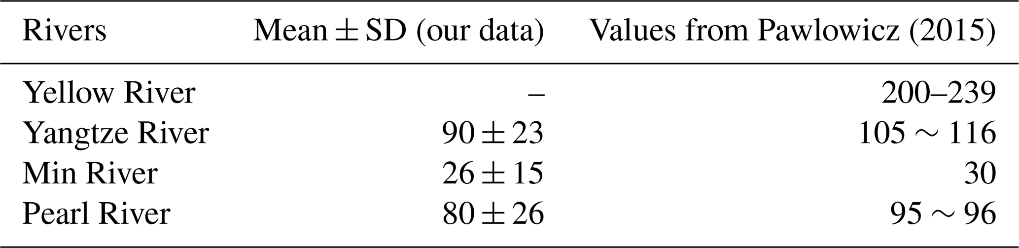
Although we have used Eq. (6), which is meant for seawater of relatively high salinity, to estimate the Absolute Salinity Anomaly near river mouths where the salinity is far smaller, a more complex calculation of the δS_A, based on a full chemical analysis of river water composition, was plotted for some of these rivers (the Yangtze, the Pearl and Min rivers) in Pawlowicz (2015). The values calculated in that work are consistent with those found here (Table 2).

Table 2 δS_A in some rivers as estimated in this paper, compared with values estimated using a more complete theory in Pawlowicz (2015). Units are milligrams per kilogram.

3.3 Parameterization of the Absolute Salinity of the China offshore waters

Although the Absolute Salinity Anomalies within rivers are always non-zero, the Absolute Salinity Anomaly is significantly non-zero in only four areas along the Chinese coast and river mouths (hatched areas in Fig. 3). They are occupied by different coastal water masses (Xiong, 2012), and the Absolute Salinities Anomalies in each can be parameterized separately.

China offshore seawater is a mixture of the Kuroshio water originating from the North Equatorial Current and the runoff into the sea. The Absolute Salinity Anomaly in Pacific surface waters in any case is generally small; it is the deeper waters that have (relatively) large Absolute Salinity Anomalies arising from remineralization in the subsurface branch of the ocean's overturning circulation. In this paper, we ignore the relative composition difference between the Kuroshio and SSW for now. Following Feistel et al. (2010b), these four water masses are regarded as the mixture of Standard Seawater that has standard-ocean salinity, with the local coastal water which contains unknown amounts of unknown solute. The related regression lines of the four water masses between Absolute Salinity Anomaly and the Reference Salinity can be computed from the samples with salinity S_R>2 g kg⁻¹, in which the seawater endpoints are chosen to be SSW with a δS_A of zero, as shown in Eq. (11) and Fig. 5.

$$\begin{array}{l}{\displaystyle }{S}_{\mathrm{A}}-S_{\mathrm{R}}=\left[\begin{array}{c}\mathrm{412}\\ \mathrm{236}\\ \mathrm{150}\\ \mathrm{107}\end{array}\right]/\left(\mathrm{mg}{\mathrm{kg}}^{-\mathrm{1}}\right)\cdot \left(\mathrm{1}-{\displaystyle \frac{S_{\mathrm{R}}}{S_{\text{SO}}}}\right),\\ \text{(11)}& {\displaystyle }\left[\begin{array}{c}\text{Laizhou Bay and Bohai Bay}\\ \text{North Jiangsu Shoal}\\ \text{Yangtze River estuary and Hangzhou Bay}\\ \text{Pearl River estuary}\end{array}\right]\end{array}$$

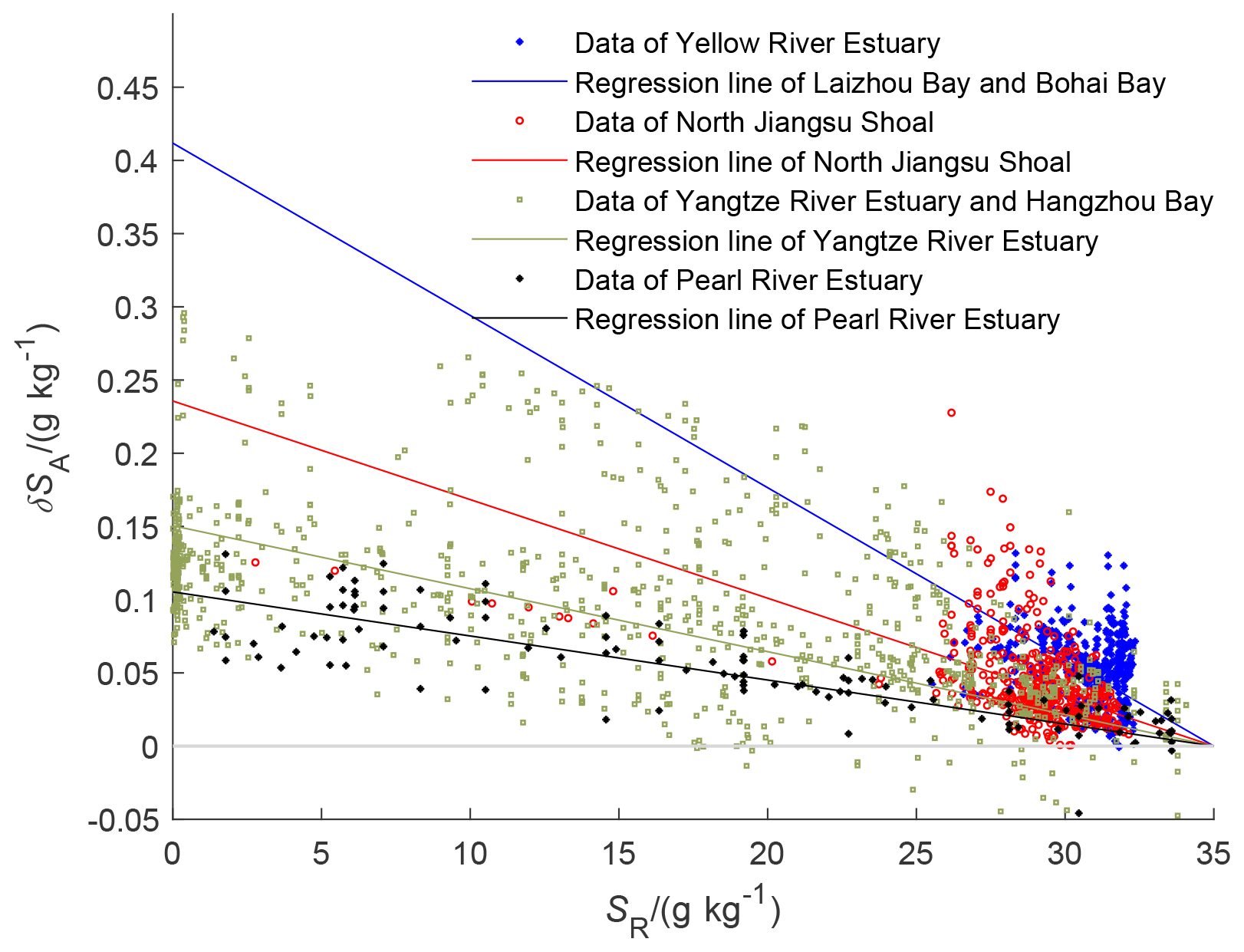
Figure 5 The Absolute Salinity Anomaly of the four regions of China offshore waters as a function of their Reference Salinity.

The linear correlation between Absolute Salinity Anomaly and S_R in the Pearl River estuary is the strongest among the four regions, which shows that the mixture between the coastal seawater and that of the open ocean is relatively conservative. There are many measurements over all salinities for the Yangtze River water. The strong scatter visible in Fig. 5 at low salinities is likely due to the rich (and highly variable) nutrient loading brought by Yangtze River draining from land.

The regressions for the two northernmost areas are less precise, as the oceanographic sampling pattern does not enter into the rivers and measured salinities are larger than 25 g kg⁻¹. The fitted curves are somewhat steeper. Note that Pawlowicz (2015) also finds that Absolute Salinity Anomalies in the Yellow River of about 0.2 g kg⁻¹ are also higher than in the other rivers (Table 2), although not as high as our fits in Fig. 5 suggest. The fit for the North Jiangsu Shoal region is heavily influenced by many high values when salinities are between 20 and 25 g kg⁻¹ and lies somewhat above a smaller number of values spread over lower salinities.

It can be seen from Fig. 5 that the relative composition anomalies decrease from north to south. The exchange of coastal waters with the open-ocean waters increases gradually from the northernmost (and somewhat enclosed) Bohai Sea estuary to the southernmost Pearl River area, which is open to the South China Sea.

3.4 Relative composition anomaly of China offshore seawater

In Eq. (6), the coefficients are determined by fitting to the results of more complete calculations that assume changes to Ca²⁺ to maintain a charge balance according to Eq. (7). We cannot directly check the accuracy of this assumption. However, Ca²⁺ was directly measured from samples in 13 cruises from April 2011 to February 2012 (Qi, 2013). Although these measurements do not occur at the same time as our larger dataset, we can group these measurements in the same regions (labeled in Fig. 1) in which we find large Absolute Salinity Anomalies. Then, we find that the ΔN[Ca²⁺], $\mathrm{\Delta }\left[{\mathrm{NO}}_{\mathrm{3}}^{-}\right]$, and Δ[NTA] (first column) values from our dataset (Table 3) are approximately consistent with Eq. (7).

Table 3 The mean value of Δ[NTA], $\mathrm{\Delta }\left[{\mathrm{NO}}_{\mathrm{3}}^{-}\right]$, Δ[NTA]^∗, and $\mathrm{\Delta }\mathrm{N}[{\mathrm{Ca}}^{\mathrm{2}+}{]}^{\ast }$ are given in different areas (marked in Fig. 1). Values obtained from Qi (2013) are labeled with “^∗”. Units are micromole per kilogram.

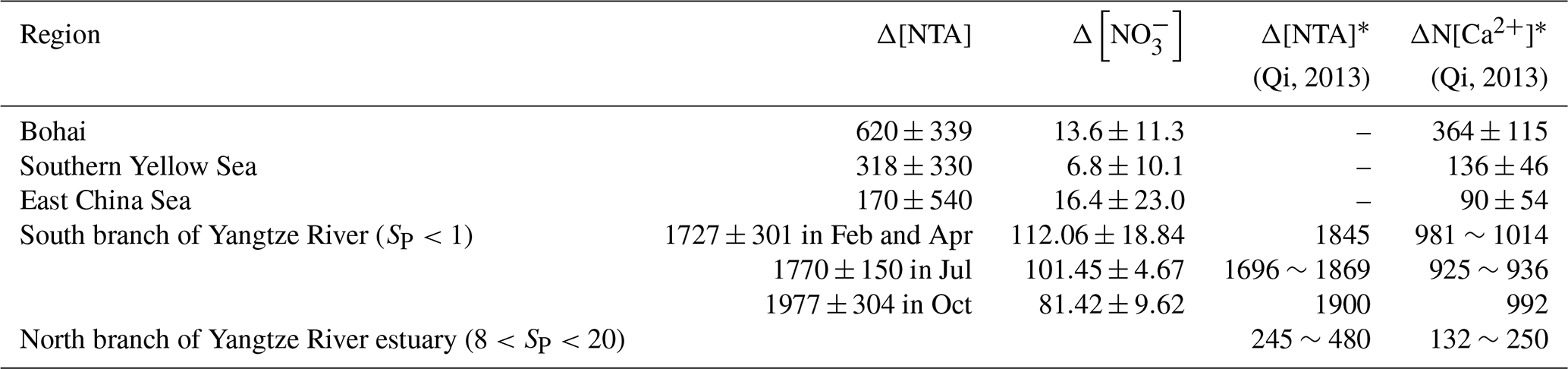
The other nutrient of phosphate is not considered in the calculation, for its concentrations range from 0 to 0.01 mmol kg⁻¹ in the existing observation, which is much smaller than those items in Eq. (7) above, and its effect is negligible. In this case, $\mathrm{\Delta }\left[{\mathrm{NO}}_{\mathrm{3}}^{-}\right]$ is mostly negligible and ΔN[Ca²⁺] is about 43 %∼58 % of Δ[NTA], in the Bohai Sear, southern Yellow Sea, East China Sea, and the Yangtze River.

The importation of Ca²⁺ and the carbon system suggest that the major source of Absolute Salinity Anomalies in shelf areas is the high CaCO₃ content of rivers. This is consistent with Absolute Salinity Anomalies in the Baltic Sea, which were found to be mostly related to the calcium carbonate input from rivers (Feistel et al., 2010a). These rivers would be the Yangtze, Yellow River, and Huai rivers. The importation fluxes of Ca²⁺ into the sea from the Yellow River and the Yangtze River are 3.6×10¹⁰ and 6.5×10¹¹ mol yr⁻¹, respectively, in 2011 (Qi, 2013). In addition, there may be re-dissolution of sediments in the Yellow River estuary and North Jiangsu Shoal. Due to the accumulation of materials entering the sea from the old Yellow River and the ancient Yangtze River, the CaCO₃ concentration of surface sediments on the seafloor of the North Jiangsu Shoal ranges from 2.8 % to 10.5 % (Qin et al., 1989; Yang and Youn, 2007). The ΔNDIC of the southern Yellow Sea near China has always been high; even when strong biological activity in spring reduces the surface Δ[NTA], the sediment of particulate inorganic carbon will resuspend and maintain the high level of dissolved CaCO₃ of seawater through the solid–liquid balance (Hong, 2012; Zhang et al., 1995).

3.5 Contrast to the δS_A calculated by GSW

Using the GSW function library and the corresponding climatological silicate and Practical Salinity data, the calculated δS_A of China offshore waters ranges from 0 to 0.002 g kg⁻¹. This is 2 orders of magnitude less than the values calculated in Sect. 3.2. The spatial distribution characteristics are also significantly different. These differences mainly come from the following aspects:

1. Instead of silicate, CaCO₃ is most likely the main relative composition anomaly of China offshore seawater and the primary contributor to the δS_A, where it is greater than 0.05 g kg⁻¹.

2. High silicate concentrations (up to 100 µmol kg⁻¹) do appear in Chinese coastal seawaters from the effects of rivers (Fig. 6), but these do not appear in the global silicate climatology used for the GSW calculations. However, even if they did, in these places Δ[NTA] is even larger, so that the effects of this coastal silicate on the Absolute Salinity Anomaly are small.

In the remaining areas, the silicate concentration is less than 20 µmol kg⁻¹, as shown in Fig. 6 at a 95 % degree of confidence; the difference between the observation and the GSW climatological dataset is [5.46, 6.21] µmol kg⁻¹, which does not change much with the seasons. It can be indicated that the GSW climatological dataset basically reflects the distribution characteristics of silicate in these areas.

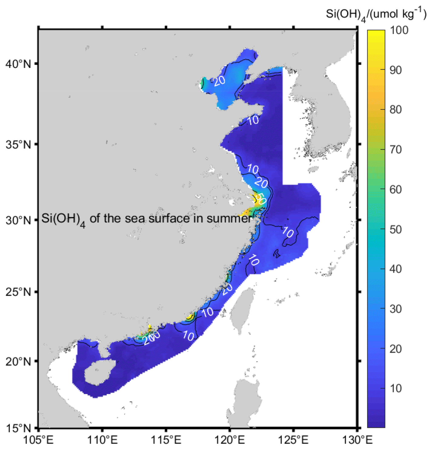
Figure 6 S_i(OH)₄ isoclines of sea surface in summer.

4 Conclusion and analysis

The proposal and implementation of the concept of S_A in TEOS-10 are meant to accurately quantify the total mass of inorganic substance dissolved in seawater, to ensure that the density and related quantities are accurately represented by the Gibbs function for seawater, and to correct errors caused by measuring the properties of seawater such as chloride and conductivity to get the salinity. In this paper, based on observations and calculations, the magnitude, distribution characteristics of Absolute Salinity in China offshore waters are described as follows:

1. The Absolute Salinity S_A ranges from 0.1 to 34.66 g kg⁻¹, in which S_R ranges from 0.01 to 34.66 g kg⁻¹, and the Absolute Salinity Anomaly δS_A ranges from −0.05 to 0.28 g kg⁻¹; this is an order of magnitude larger than the largest values in the open ocean.

2. The largest δS_A values are located in four distinct regions: the Yangtze River mouth/Hangzhou Bay, the North Jiangsu Shoal, the Bohai Sea, and the Pearl River mouth, all of which are areas where the Δ[NTA] is high.

3. Instead of silicate, CaCO₃ is most likely the main composition anomaly relative to SSW and the primary contributor to the δS_A in the above four areas.

4. Under the combined effects of different water system dynamics, terrestrial input, marine biological activities, and re-dissolution of marine sediments, the δS_A values in China offshore waters' seasonal variations are obvious, and the maximum can be as high as 0.05 g kg⁻¹; the difference between the surface layer and the bottom layer is also up to 0.1 g kg⁻¹.

With the observations available, this paper only lists the magnitude and distribution characteristics of δS_A in China offshore waters from 2006 to 2007, although it is likely that similar features will occur in other years. At present, we have collated the long-term series of seawater composition data to continue the study on δS_A changes and get an empirical formula to calculate δS_A.

The current research is only based on the existing seawater composition data, and the exact influence of other changes to composition is still not very clear. To verify these findings, a complete chemical analysis and/or direct measurements of seawater density would be useful in the estuaries of the Yangtze River, Qiantang River, Pearl River, Min River, and the semi-enclosed Bohai Sea.