the Creative Commons Attribution 4.0 License.
the Creative Commons Attribution 4.0 License.
 | 01 Jul 2021
Tropical deoxygenation sites revisited to investigate oxygen and nutrient trends
Lothar Stramma
An oxygen decrease of the intermediate-depth low-oxygen zones (300 to 700 m) is seen in time series for selected tropical areas for the period 1960 to 2008 in the eastern tropical Atlantic, the equatorial Pacific and the eastern tropical Indian Ocean. These nearly 5-decade time series were extended to 68 years by including rare historic data starting in 1950 and more recent data. For the extended time series between 1950 and 2018, the deoxygenation trend for the layer 300 to 700 m is similar to the deoxygenation trend seen in the shorter time series. Additionally, temperature, salinity, and nutrient time series in the upper-ocean layer (50 to 300 m) of these areas were investigated since this layer provides critical pelagic habitat for biological communities. Due to the low amount of data available, the results are often not statistically significant within the 95 % confidence interval but nevertheless indicate trends worth discussing. Generally, oxygen is decreasing in the 50 to 300 m layer, except for an area in the eastern tropical South Atlantic. Nutrients also showed long-term trends in the 50 to 300 m layer in all ocean basins and indicate overlying variability related to climate modes. Nitrate increased in all areas. Phosphate also increased in the Atlantic Ocean and Indian Ocean areas, while it decreased in the two areas of the equatorial Pacific Ocean. Silicate decreased in the Atlantic and Pacific areas but increased in the eastern Indian Ocean. Hence, oxygen and nutrients show trends in the tropical oceans, though nutrients trends are more variable between ocean areas than the oxygen trends; therefore, we conclude that those trends are more dependent on local drivers in addition to a global trend. Different positive and negative trends in temperature, salinity, oxygen and nutrients indicate that oxygen and nutrient trends cannot be completely explained by local warming.
- Article
(3673 KB) - Full-text XML
-
Supplement
(88 KB) - BibTeX
- EndNote


Temperature, oxygen and nutrient changes in the ocean have various impacts on the ecosystem. These impacts span from habitat compression in the open ocean (Stramma et al., 2012) and affect all marine organisms through multiple direct and indirect mechanisms (Gilly et al., 2013) to affect the ecophysiology of marine water-breathing organisms with regard to distribution, phenology and productivity (Cheung et al., 2013). Despite its far-reaching consequences for humanity, the focus on climate change impacts on the ocean lags behind the concern for impacts on the atmosphere and land (Allison and Bassett, 2015). An oceanic increase in stratification and thus reduction in ventilation and decrease in oceanic dissolved oxygen are two of the less obvious but important expected indirect consequences of climate change on the ocean (Shepherd et al., 2017). Warming leads to lighter water in the surface layer and increased stratification, reducing the mixing and deep ventilation of oxygen-rich surface water to the subsurface layers. Increasing ocean stratification over the last half century of about 5 % is observed in the upper 200 m (Li et al., 2020). The subsequent previously observed deoxygenation (e.g., Stramma et al., 2008; Schmidtko et al., 2017) of the open ocean is one of the major manifestations of global change. This temperature oxygen relation can also be seen for the 0–1000 m layer of the global ocean, as the oxygen inventory is negatively correlated with the ocean heat content (; 0–1000 m) (Ito et al., 2017). Oxygen-poor waters, often referred to as oxygen minimum zones (OMZ), occupy large volumes of the intermediate-depth eastern tropical oceans. In an investigation of six selected areas for the 300 to 700 m layer in the tropical oceans for the time period 1960 to 2008, Stramma et al. (2008) observed declining oxygen concentrations of −0.09 to −0.34 µmol kg−1 yr−1 and a vertical expansion of the intermediate-depth low-oxygen zone. Such a vertical expansion of the OMZ that is entered and passed by diel vertical migrators and sinking particles could have widespread effects on species distribution, the biological pump and benthic–pelagic coupling (Wishner et al., 2013). The areas of the world ocean investigated for oxygen changes can be extended and placed in a quantitative assessment of the entire world ocean oxygen inventory by analyzing dissolved oxygen and supporting data for the complete oceanic water column over the past 50 years since 1960. Schmidtko et al. (2017) reported that the global oceanic oxygen content of 227.4 ± 1.1 Pmol (1015 mol) has decreased by more than two percent (4.8 ± 2.1 Pmol). However, these oxygen changes vary by region, with some areas showing increasing oxygen values on timescales related to climate modes.
The nutrient distribution is, in addition to oxygen, a key parameter controlling the marine ecosystems. However, very little is known about long-term nutrient changes in the ocean. The transformation of carbon and nutrients into organic carbon, its sinking, advection and subduction into the in the deep ocean, and its decomposition at depth, is known as the biological carbon pump. As a consequence, nutrients are consumed and are thus lower in the surface ocean and higher in the deep ocean. The oceanic distribution of nutrients and patterns of biological production are controlled by the interplay of biogeochemical and physical processes, and external sources (Williams and Follows, 2003). In the upper 500 to 1000 m of the tropical oceans the nutrient concentration is higher than in the subtropics and is decreasing westwards (Levitus et al., 1993). In the subarctic North Pacific, surface nutrient concentration decreased during 1975 to 2005 and is strongly correlated with a multidecadal increasing trend of sea surface temperature (SST) (Ono et al., 2008). Below the surface, however, oxygen decreased and nutrients increased in the subarctic Pacific pycnocline from the mid-1980s to around 2010 (Whitney et al., 2013). Nutrients would be expected to vary inversely with oxygen if the dominant process was the remineralization of marine detritus (Whitney et al., 2013). In a recent study, the trends of nutrients in the open Pacific Ocean were investigated (Stramma et al., 2020), and in the open Pacific Ocean nutrient trends were observed and seemed to be related to oxygen trends. The supply of nutrients to the sunlit surface layer of the ocean has traditionally been attributed solely to vertical processes. However, horizontal advection may also be important in establishing the availability of nutrients in some regions. Palter et al. (2005) showed that the production and advection of North Atlantic Subtropical Mode Water introduces spatial and temporal variability in the subsurface nutrient reservoir beneath the North Atlantic subtropical gyre. By means of a coupled ecosystem circulation model Oschlies (2001) described for the North Atlantic that the long-term change in the North Atlantic Oscillation (NAO; e.g., Hurell and Deser, 2010) between the 1960s and 1990s may have induced significant regional changes in the upper ocean's nutrient supply. These include a decrease of nitrate supply to the surface waters of by about 30 % near Bermuda and in midlatitudes and a simultaneous 60 % increase to nitrate flux in the upwelling region off West Africa. On the other side of the globe, the Indonesian throughflow (ITF) is a choke point in the upper-ocean thermohaline circulation, carrying Pacific waters through the strongly mixed Indonesian seas and into the Indian Ocean (Ayers et al., 2014). Ayers et al. (2014) determined the depth- and time-resolved nitrate, phosphate and silicate fluxes at the three main exit passages of the ITF: the Lombok Strait, Ombai Strait and Timor Passage. Nutrient flux, as well as its variability with depth and time, differed greatly between the passages. They estimated the effective flux of nutrients into the Indian Ocean and found that the majority of ITF nutrient supply to the Indian Ocean is to thermocline waters, where it is likely to support new production and significantly impact Indian Ocean biogeochemical cycling.
Here we investigate the extent of changes in oxygen, temperature, and salinity trends for the six tropical areas with longer time series compared to the previously time series, which was about one-third shorter. In addition, trends in the biologically active near-surface layer (50 to 300 m) are investigated. As the upper ocean provides critical pelagic habitat for biological communities, nutrient time series of the six tropical areas since 1950 are investigated at 50 to 300 m depth, as nutrient changes in combination with hydrographic changes will influence the biological productivity of the ocean (Sigman and Hain, 2012). The upper boundary of 50 m was chosen to reduce the influence of the seasonal cycle in the upper 50 m although the seasonal cycle in the tropics is weaker than in most subtropical and subpolar regions (Louanchi and Najjar, 2000). However, the thermocline shift could be due to ocean warming and various climate modes, the averaging across the depths could lead to an influence on the trend of the 50 to 300 m layer.
Stramma et al. (2008) investigated the temperature and oxygen trends for the period 1960 to 2008 in the 300 to 700 m layer of six tropical ocean areas. There were three areas in the tropical Atlantic (A: 10–14∘ N, 20–30∘ W; B: 3∘ S–3∘ N, 18–28∘ W; C: 14∘ S–8∘ S, 4–12∘ E), two areas in the eastern and central tropical Pacific (D: 5∘ S–5∘ N, 105–115∘ W; E: 5∘ S–5∘ N, 165–175∘ W), and one in the eastern Indian Ocean (F: 5∘ S–0∘ N, 90–98∘ E) (Fig. 1). Here these time series were extended with more recent data and back in time to 1950 for the regions with available data (Table 1 and Fig. 2).
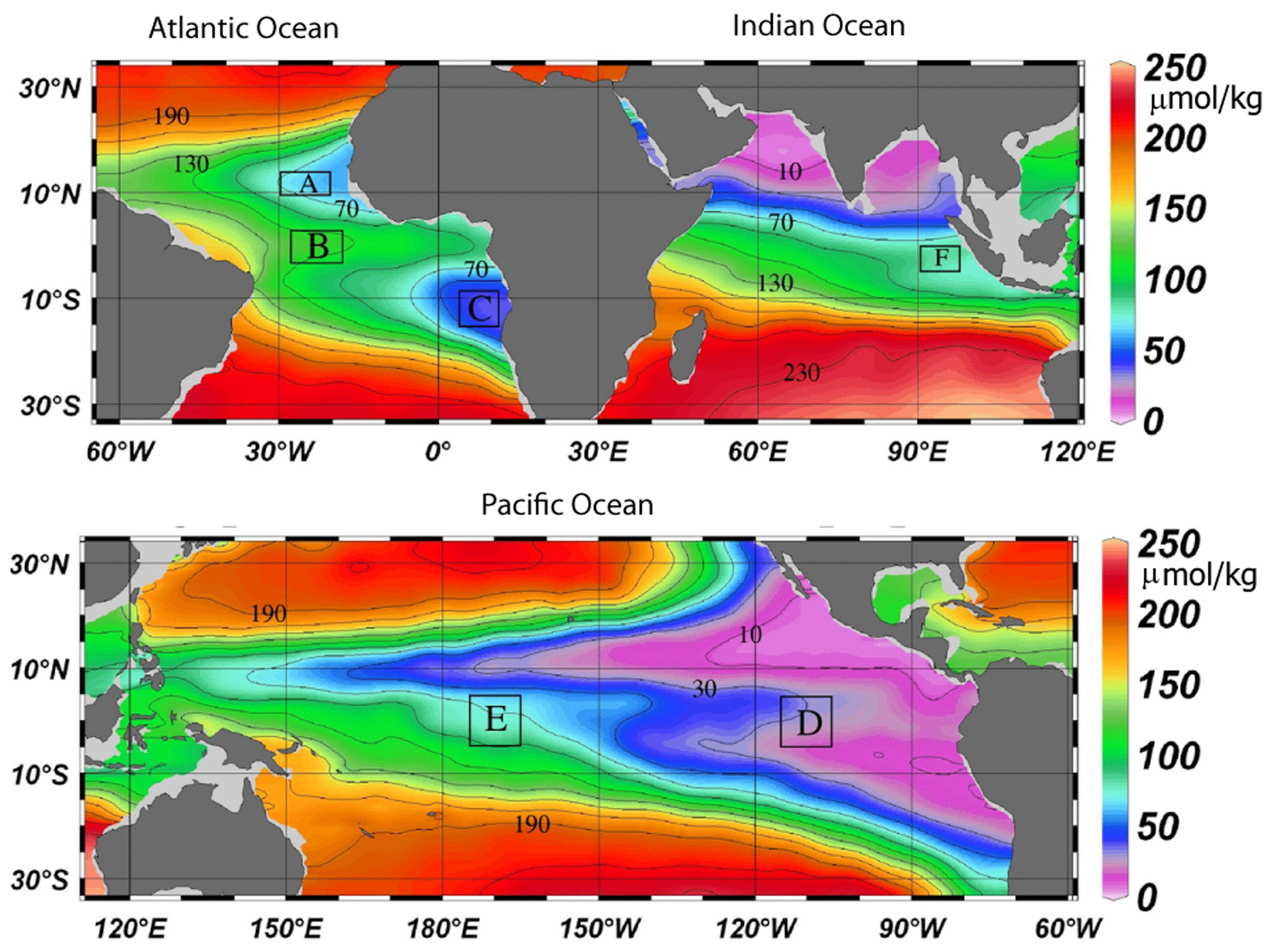
Figure 1Climatological mean dissolved oxygen concentration (µmol kg−1, shown in color) at 400 m depth contoured at 20 µmol kg−1 intervals from 10 to 230 µmol kg−1 (black lines). Analyzed areas A to F (Table 1) are enclosed by black boxes (Stramma et al., 2008).
Despite long-term trends in ocean oxygen, climate-signal-related influence on the trends was also observed in recent years. More recently, long-term trends and climate-signal-related influence were also observed for nutrients. The areas D and E were also used for the layer 50 to 300 m for oxygen changes in Stramma et al. (2020) but not for nutrient trends due to the low amount of available nutrient data. However, here we also list the nutrients trends for these two areas, despite the fact that the low amount of data does not make these calculations statistically significant (Table 2).
The main hydrographic data set is similar to the one used and described in Schmidtko et al. (2017), relying on Hydrobase 2 and World Ocean Database bottle data for nutrient data. Quality control and handling is described in Schmidtko et al. (2017) for oxygen and is used here similarly for nutrients. Summarizing the most important steps, only profiles with plausible values were used, profiles with linear or constant values over depths were removed, duplicates detected within 5 km and 25 h used the one with best vertical resolution, database control flags were observed, and a minimum divergence of values was required. The only divergence to the described procedure is that bottle data with missing temperature and/or salinity were assigned the temporal and spatial interpolated temperature and salinity derived from MIMOC (Schmidtko et al., 2013). This was done to ensure that all data were in units of µmol kg−1 and did not require the discarding of already sparse data due to missing water density (temperature and salinity) values. This enables us to use data provided in the databases in mol L−1 or mL L−1 that otherwise could not be used.
As a main focus of the computations is the comparison with the results of Stramma et al. (2008), we applied similar methods for a direct comparison. All data from bottle as well as CTD measurements within a selected area sampled within 1 year were combined independent of the season and location and then used for the trend computation. As in Stramma et al. (2008), the amount of data was too small to further distinguish for season and location within the area. Profiling float data were not used as oxygen measurements on our floats and showed drifts in time, probably due to biological activity on the sensors, which could lead to biased trends. Earlier measurements from bottle data had less accurate depth measurements and fewer vertical measurements compared to years with CTD profiles within the selected depth layers. This can add some uncertainty to earlier measurements, though no systematic bias towards increasing or decreasing oxygen trends. For years with CTD measurements on 1 dbar (10 kPa) steps, the uncertainties between years will be less significant than those years with only bottle data. Mean parameter values for each layer were computed from the annual mean values in the selected depth layer. The standard deviation of the parameter values depends both on the variability of the annual mean parameter value and the strength of the trend during the measurement period.
In the Atlantic the hydrographic and nutrient data were extended with some RV Meteor, RV Merian and RV Poseidon cruises. For area A, data from Meteor cruises M68/2 (2006), M83/1 (2008), M97 (2010), M119 (2015), and M145 (2018) and Merian MSM10/1 (2008) were added. For area B, Meteor cruises M106 (2014), M130 (2016) and M145 (2018) were added. For area C, cruise data from Poseidon P250 (1999), Merian MSM07 (2008), Meteor M120 (2015), Meteor M131 (2016), and Meteor M148 (2018) were included.
In the Pacific, the region at 5∘ N–5∘ S, 165–175∘ W (area E), which had data until 2009, was supplemented with data from an RV Investigator cruise at 170∘ W from June 2016. The region 5∘ N–5∘ S, 105–110∘ W (area D), which had data up to 2008, was supplemented with data from an RV Ron Brown cruise at 110∘ W in December 2016.
Climate indices considered include the NAO, the Atlantic Multidecadal Oscillation (AMO), the Pacific Decadal Oscillation (PDO), El Niño–Southern Oscillation (ENSO) and the Indian Ocean Dipole Mode (IOD). The NAO is an extratropical climate signal of the North Atlantic. As our areas are tropical regions, the three Atlantic areas were investigated relative to the AMO index (Montes et al., 2016) before and after 1995. The AMO was high before 1963, low until 1995, and has been high since 1995. In the Pacific, the central equatorial area at 5∘ N–5∘ S, 165–175∘ W (area E in Stramma et al., 2008), which had hydro-data until 2009, was supplemented with data from an RV Investigator cruise at 170∘ W from June 2016. The eastern equatorial area 5∘ N–5∘ S, 105–115∘ W (area D in Stramma et al., 2008), which had hydro-data until 2008, was supplemented with data from an RV Ron Brown cruise at 110∘ W in December 2016. The data were investigated in relation to the PDO (e.g., Deser et al., 2010) before and after 1977. The PDO was negative from 1944 to 1976, positive from 1977 to 1998, variable from 1998 to 2013 and positive after 2013. In the Indian Ocean the available data covered area F only after 1960 but until 2016. Area F (0–5∘ S, 90–98∘ E) is shown in relation to the IOD (Saji et al., 1999), which slightly increased after 1990.
Linear trends and their 95 % confidence interval were computed by using annual averages (all measurements within 1 year were attributed to that year) of the profiles linearly interpolated to standard 5 dbar spaced depth levels. A computation routine was used to derive the effective number of degrees of freedom for the computation of the confidence interval. The data used for the oxygen time series were interpolated to 5 dbar steps with an objective mapping scheme (Bretherton et al., 1976) with Gaussian weighting. In the 50 to 300 m and the 300 to 700 m layers, a temporal half folding range of 0.5 year and a vertical half folding range of 50 m with maximum ranges of 1 year and 100 m, respectively, were applied. The covariance matrix was computed from the closest 100 local data points and 50 random data points within the maximum range, for the diagonal of the covariance matrix a signal to noise ratio of 0.7 was set (see Schmidtko et al., 2013, for details). A more improved mapping scheme was used compared to the one used in Stramma et al. (2008) where larger temporal ranges were used (1 year half folding and a maximum temporal range of 2 years).
The nutrients nitrite (NO, nitrate (NO, phosphate (PO and silicic acid (Si(OH)4 referred to as silicate hereafter) on the recent cruises were measured on board with a QuAAtro auto-analyzer (Seal Analytical). For recent auto-analyzer measurements the precision is 0.01 µmol kg−1 for phosphate, 0.1 µmol kg−1 for nitrate, 0.5 µmol kg−1 for silicate and 0.02 mL L−1 (∼ 0.9 µmol kg−1) for oxygen from Winkler titration (Bograd et al., 2015). For older uncorrected nutrient data, offsets are estimated to be 3.5 % for nitrate, 6.2 % for silicate, and 5.1 % for phosphate (Tanhua et al., 2010). One problem with nutrient data is that certified reference material (CRM) was applied to some measurements while for other measurements only a bias was applied. Inter-cruise offsets were investigated for the deep ocean between WOCE (World Ocean Circulation Experiment) and non-WOCE cruises and resulted in root-mean-square inter-cruise offsets before adjustment of 0.003 g kg−1 for salinity, 2.498 µmol kg−1 for oxygen, 2.4 µmol kg−1 for silicate, 0.55 µmol kg−1 for nitrate and 0.045 µmol kg−1 for phosphate (Gouretski and Jancke, 2001), while Johnson et al. (2001) presented initial standard deviations of crossover differences of WOCE cruises of 0.0028 for salinity, 2.1 % for oxygen, 2.8 % for nitrate, 1.6 % for phosphate, and 2.1 % for silicic acid. Hence, a slight bias based on the measurements applied could be included in the measurements.
The ENSO cycle of alternating warm El Niño and cold La Niña events is the climate system's dominant year-to year signal. ENSO originates in the tropical Pacific through interaction between the ocean and the atmosphere, but its environmental and socioeconomic impacts are felt worldwide (McPhaden et al., 2006). The 3-month running mean SST anomalies (ERSST.v5 SST anomalies) in the Niño 3.4 region (equatorial Pacific: 5∘ N to 5∘ S, 120 to 170∘ W) of at least +0.5 ∘C and lasting for at least five consecutive 3-month periods are defined as El Niño events, and five consecutive 3-month periods of at least −0.5 ∘C are defined as La Niña events (http://origin.cpc.ncep.noaa.gov/products/analysis_monitoring/ensostuff/ONI_v5.php, last access: 14 June 2021). In case of measurements in ENSO years in Figs. 3, 4 and 5, the very strong El Niño events of 1983, 1998 and 2015 and the strong El Niño events 1957, 1965, 1972, 1987 and 1991 are marked by red circles, and the strong La Niña events 1974, 1976, 1989, 1999, 2000, 2007 and 2010 are marked by blue squares. A shoaling thermocline, such as what occurs in the eastern Pacific during La Niña or cool (negative) PDO states, enhances nutrient supply and organic matter export in the eastern Pacific while simultaneously increasing the fraction of that organic matter that is respired in the low-oxygen water of the uplifted thermocline. The opposite occurs during El Niño or a warm (positive) PDO state; a deeper thermocline reduces both export and respiration in low-oxygen water in the eastern Pacific, allowing the hypoxic water volume to shrink (Deutsch et al., 2011; Fig. S7). ENSO also has some influence on the tropical Atlantic Ocean and Indian Ocean. The equatorial Atlantic oscillation is influenced by the Pacific ENSO with the equatorial Atlantic sea surface temperature lagging by about 6 months (Latif and Grötzner, 2000). In the Indian Ocean there has been a recent weakening of the coupling between the ENSO and the IOD mode after the 2000s and 2010s compared to the previous 2 decades (1980s and 1990s) (Ham et al., 2017).
3.1 Trends in the 300 to 700 m depth layer
Nutrient data are sparse in the deeper part of the ocean and are less important than the near-surface layer for the marine ecosystems and therefore are not presented here for the 300 to 700 m depth layer. Oxygen trends for the period 1960 to 2008 for the 300 to 700 m layer of the six areas investigated (Stramma et al., 2008) for the tropical oceans were all negative in the range −0.09 to −0.34 µmol kg−1 yr−1 (Table 1). For the extended time period between 1950 and 2018, the oxygen trends were in the same order of magnitude for the areas A to F in the range −0.11 to −0.27 µmol kg−1 yr−1 (Table 1). The 1950 to 2018 temperature trends were positive in the three Atlantic areas and the eastern tropical Pacific but negative in the central Pacific Ocean and Indian Ocean areas (Table 1). In the eastern tropical Pacific (area D) and the eastern Indian Ocean (area F) there was even a reversed trend in temperature compared to the shorter time period between 1960 and 2008, although all temperature trends are not within the 95 % confidence interval difference from 0. The salinity of the 300 to 700 m layer increased for the Atlantic Ocean and Indian Ocean areas and decreased in the two Pacific areas (Table 1).
Table 1Linear trends (300 to 700 m) of temperature in ∘C yr−1, oxygen in µmol kg−1 yr−1 and salinity yr−1 with 95 % confidence intervals (p values) where data are available for the entire period listed. Trends whose 95 % confidence interval includes zero are shown in bold. Trends computed in Stramma et al. (2008) are shown for comparison.
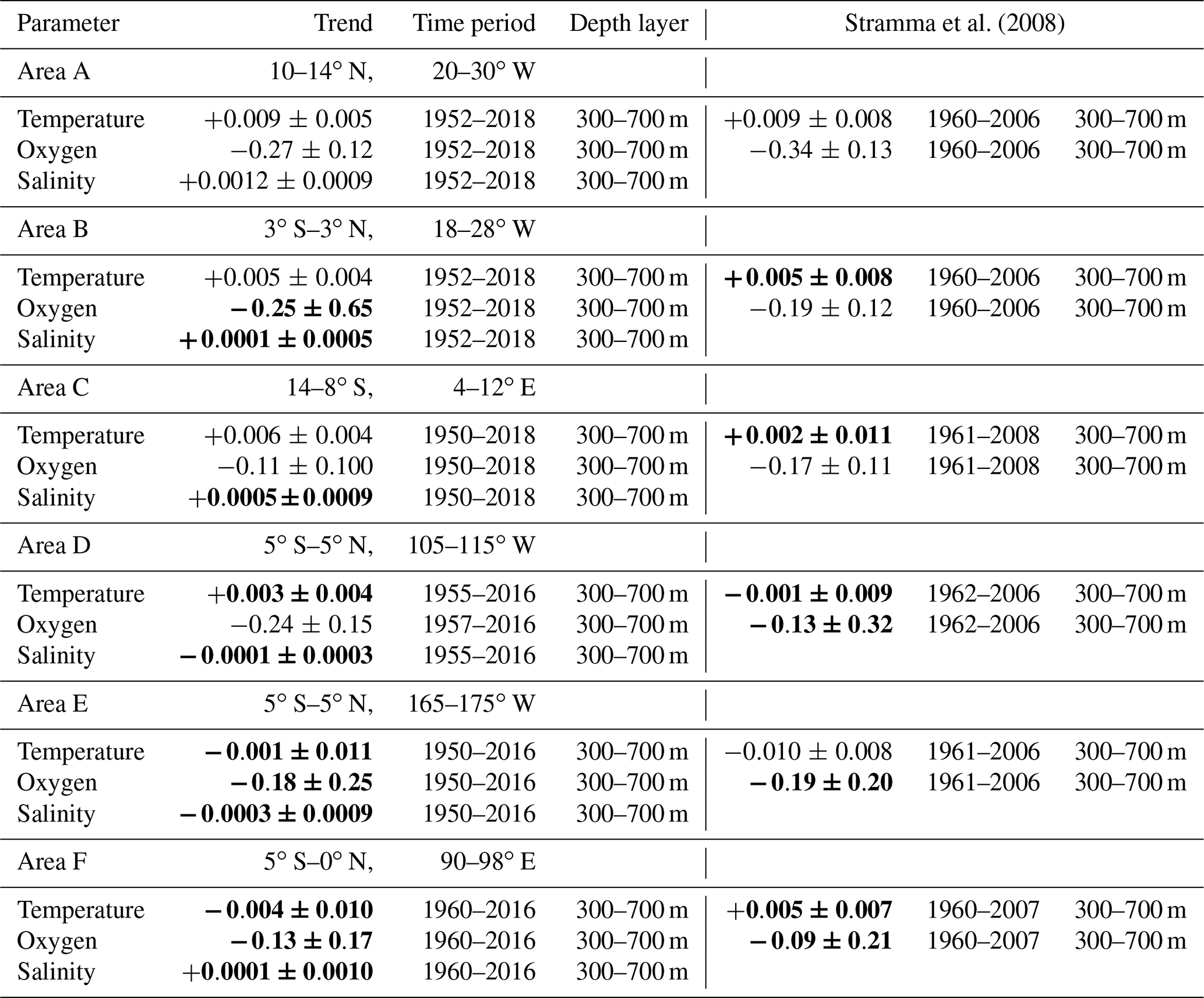
For the area A (10–14∘ N, 20–30∘ W) the oxygen trend for 300 to 700 m for the period 1952 to 2018 (Fig. 2a) was weaker ( µmol kg−1 yr−1) than for the period 1960 to 2006 ( µmol kg−1 yr−1). In the western subtropical and tropical Atlantic oxygen measurements from time series stations and shipboard measurements showed a significant relationship with the wintertime AMO index (Montes et al., 2016). During negative wintertime AMO years trade winds are typically stronger and these conditions stimulate the formation and ventilation of Subtropical Underwater (Montes et al., 2016) with higher oxygen content. Even in the 300 to 700 m layer of Area A (Fig. 2a), as well as the 50 to 300 m layer (Fig. 3a), the oxygen content is higher during the negative AMO period and lower during the positive AMO phase. For a section along 23∘ W between 6–14∘ N from 2006 to 2015 crossing area A, an oxygen decrease in the 200 to 400 m layer and an increase in the 400 to 1000 m layer was described (Hahn et al., 2017), which can not be confirmed in area A due to the different geographical and temporal boundaries and the variable annual mean oxygen values after 2006 in area A.
The 1952 to 2018 oxygen trend in the equatorial Atlantic (area B) shows a large 95 % confidence interval, different to the shorter time period 1960 to 2006 (Table 1). The larger confidence interval is caused by a low oxygen concentration in 1952 and large variability after 2006 (Fig. 2b). The equatorial Atlantic in the depth range 500 to 2000 m is influenced by Equatorial Deep Jets, with a periodically reversing flow direction influencing the transport of oxygen (Bastin et al., 2020), which might be one reason for the large oxygen variability. During the negative AMO, the oxygen trend was slightly positive ( µmol kg−1 yr−1) but negative after 1995 (Fig. 2b).
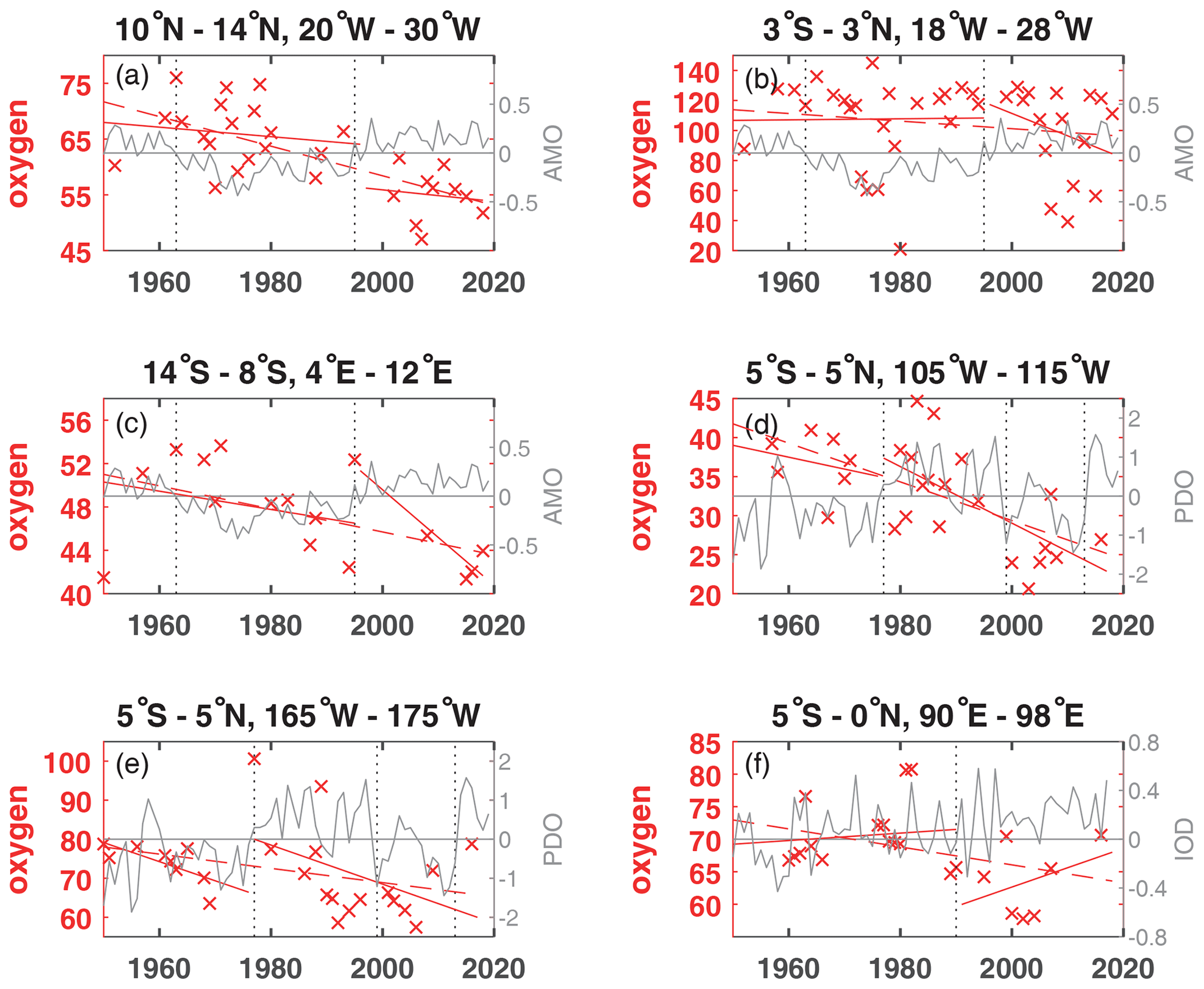
Figure 2Annual mean oxygen concentration for the years available (×) used to calculate trends for the layer 300 to 700 m in µmol kg−1 plotted for the available years in the time period 1950 to 2018 (dashed red line) and for the positive and negative periods of the AMO in the Atlantic (a–c), the PDO in the Pacific (d, e), and the IOD in the Indian Ocean (f) as solid red lines. The AMO, PDO and IOD are shown as grey lines. The change of AMO status in 1963 and 1995; the change of the PDO phase in 1977, 1999, and 2013; and the IOD in 1990 are marked by dotted vertical lines. The scale of the y axis changes according to the oxygen concentration of each area.
The area C in the eastern tropical South Atlantic shows similar positive trends in temperature and salinity (Table 1) as in the two other Atlantic areas investigated. Area C is located in the region with the lowest oxygen content in the Atlantic Ocean (Fig. 1). Due to the already low oxygen concentration in this region, the decrease in oxygen is weaker than in the two other Atlantic Ocean areas in the period 1950 to 2018, similar to the weaker decrease in area C for the shorter time period 1961 to 2008 (Table 1). Higher oxygen concentrations were also seen in the few oxygen profiles in area C during the negative AMO and lower oxygen concentrations were measured after the year 2000 (Fig. 2c).
In the equatorial Pacific the two areas show a clear long-term oxygen decrease in the 300 to 700 m layer but no clear changes related to the PDO phases before and after 1977 (Fig. 2d, e). However, the PDO index after 1977 was mainly positive until 1999 and mainly negative between 1999 and 2013. In cases where these time periods are looked at separately, the oxygen concentration was higher during the period 1977 to 1990 and lower during 1999 to 2010, as expected for the PDO influence (e.g., Deutsch et al., 2011).
In the eastern Indian Ocean, the 300 to 700 m oxygen concentration was lower for the slightly positive IOD phase after 1990, leading to a long-term oxygen concentration decrease in area F. However, the trends for the shorter periods prior to 1990 and after 1990 showed a positive oxygen trend (Fig. 2f), which is caused by high oxygen concentrations near the end of both measurement periods. The temperature in this area decreased and salinity showed barely any change (Table 1); hence, the oxygen decrease is not coupled to temperature or hydrographic water mass changes.
3.2 Trends in the 50 to 300 m layer
The trend computations for the layer 50 to 300 m for temperature, salinity, oxygen and nutrients (Table 2) show different trends for the selected areas in the three tropical oceans. Since this layer is close to the thermocline, oxycline and nutricline, some noise in the data could originate from sampling close to these gradients. In the near-surface layer (50 to 300 m) the long-term oxygen trends were negative as they were in the deeper layer (300 to 700 m), except for area C in the eastern tropical South Atlantic (Fig. 3c). However, this oxygen trend in area C is not stable due to the large variability in the time period 1960 to 1990. The upper layer of the area C is influenced by the Angola Dome centered at 10∘ S, 9∘ E (Mazeika, 1967), which might influence the larger variability near the surface. Area C shows the largest mean nitrate, silicate and phosphate concentrations in the Atlantic in the 50 to 300 m layer and the 300 to 700 m layer (Table 3) and shows the large nutrient availability in the eastern tropical South Atlantic. At 250 and 500 m depth, the region of area C was shown to have the highest nitrate and phosphate concentrations of the tropical and subtropical Atlantic Ocean (Levitus et al., 1993). It was observed that in the Pacific Ocean nutrients are related to oxygen changes and climate variability (Stramma et al., 2020). The ENSO signal was apparent in most cases, as in the tropical Atlantic Ocean and Indian Ocean (Nicholson, 1997); hence, the oxygen distribution for the layer 50 to 300 m (Fig. 3) is marked for El Niño and La Niña events to check for the possible influence of ENSO in the shallow depth layer. Most of the nutrient trends are due to sparse data coverage and are thus not statistically significant; nevertheless, it is insightful to compare the nutrient trends with the oxygen trends and the climate signals.
Table 2Linear trends (50–300 m) of temperature (∘C yr−1), salinity (yr−1) and solutes (µmol kg−1 yr−1) with 95 % confidence intervals (p values) where data are available for the entire period 1950 to 2018 (left rows) and for the earlier time period (center rows) and later time period (right rows) separated in 1995 in the Atlantic Ocean (areas A, B, C), in 1977 in the Pacific Ocean (areas D, E) and in 1990 in the Indian Ocean (area F). Trends whose 95 % confidence interval includes zero are shown in bold.
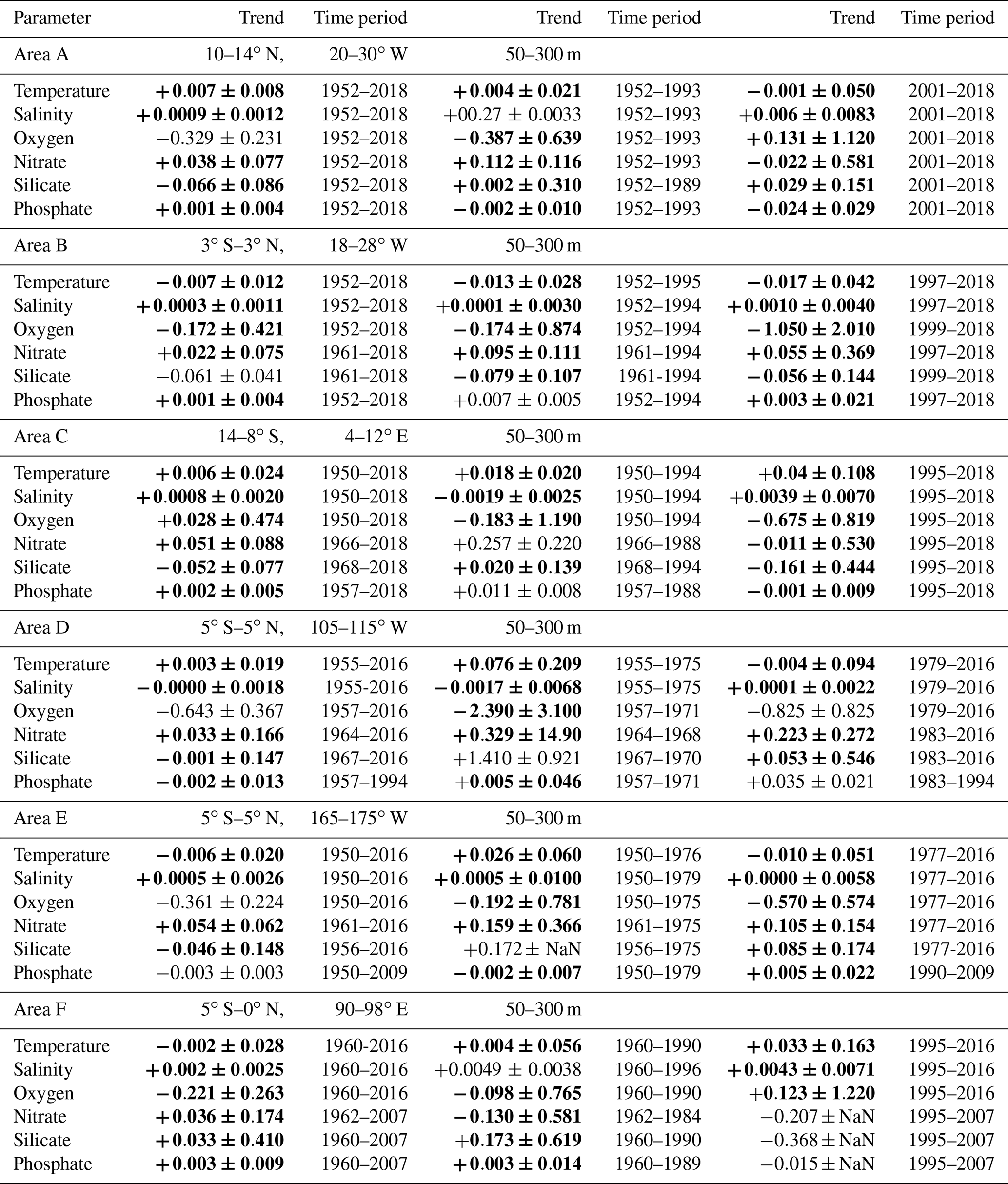
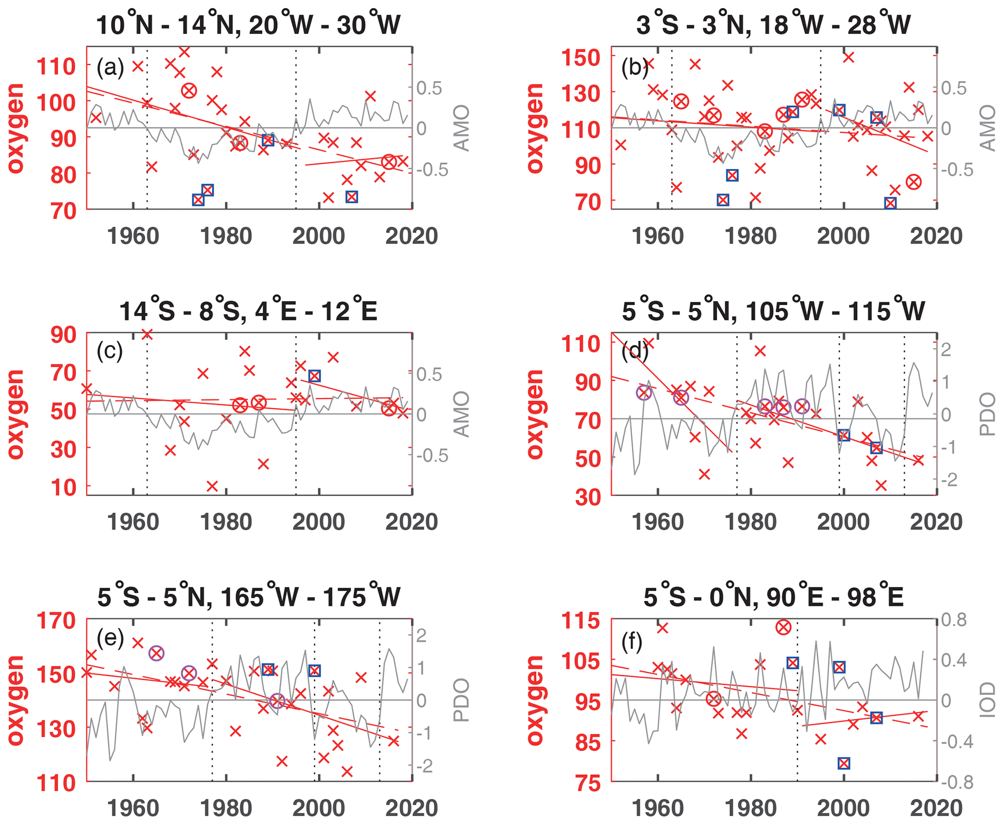
Figure 3Annual mean oxygen concentration for years available (×) used to calculate trends for the layer 50 to 300 m in µmol kg−1 plotted for the available years in the time period 1950 to 2018 (dashed red line) and for the positive and negative periods of the AMO in the Atlantic (a–c), the PDO in the Pacific (d, e) and the IOD in the Indian Ocean (f) as solid red lines. The AMO, PDO and IOD are shown as grey lines. The change of AMO status in 1963 and 1995; the change of the PDO phase in 1977, 1999, and 2013; and the IOD in 1990 are marked by dotted vertical lines. El Niño years defined as strong are marked by an additional magenta circle, and strong La Niña years are marked by an additional blue square. The scale of the y axis changes according to the oxygen concentration range of each area.
Table 3Mean parameter values with number of profiles and standard deviation for the time period covered derived from the annual mean parameter value in brackets for the layers 50–300 and 300–700 m of temperature (∘C), salinity and solutes (µmol kg−1) in the Atlantic Ocean (areas A, B, C), in the Pacific Ocean (areas D, E) and in the Indian Ocean (area F).
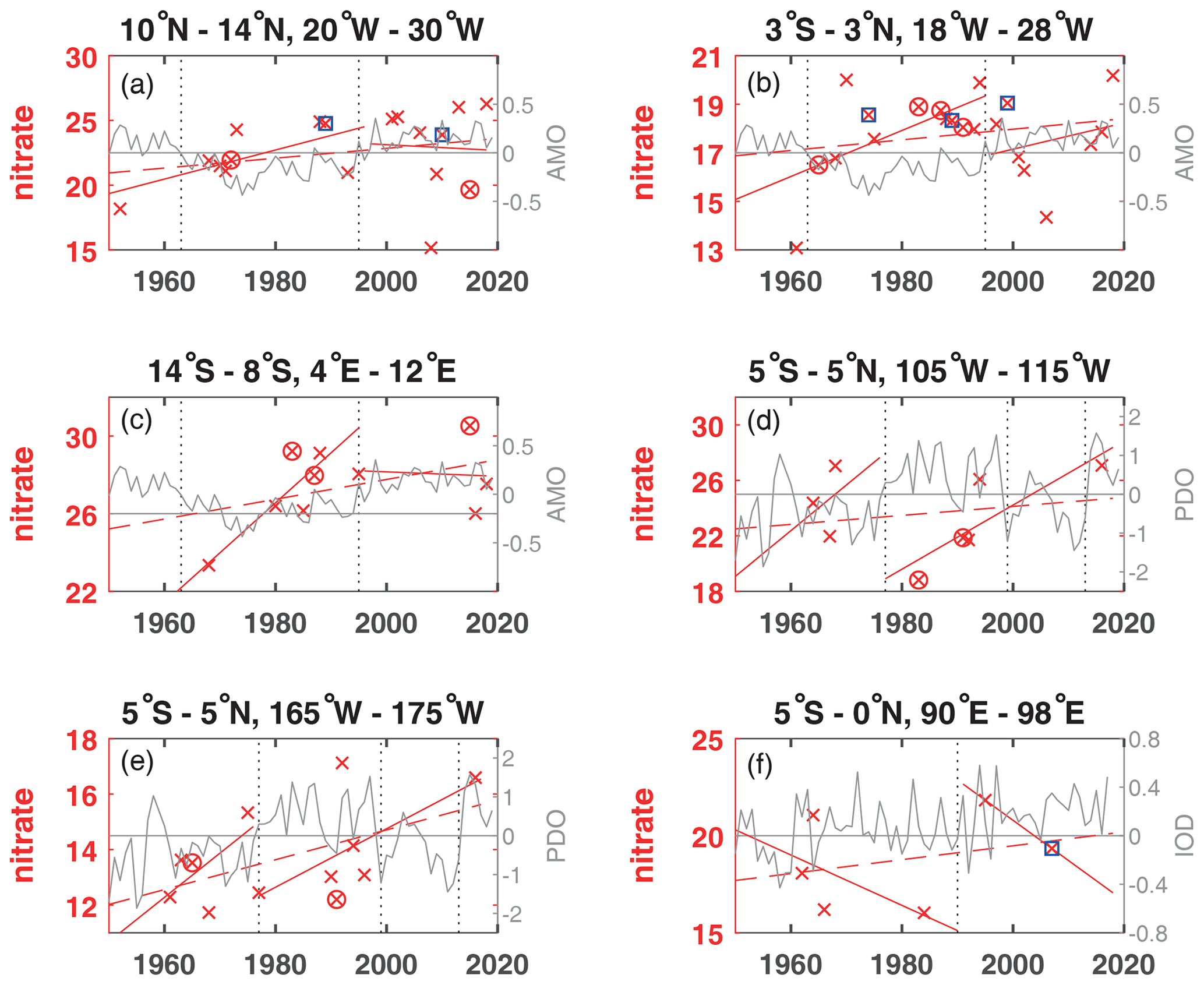
Figure 4Annual mean nitrate concentration for years available (×) used to calculate trends for the layer 50 to 300 m (µmol kg−1) plotted for the available years in the time period 1950 to 2018 (dashed red line) and for the positive and negative periods of the AMO in the Atlantic (a–c), the PDO in the Pacific (d, e) and the IOD in the Indian Ocean (f) as solid red lines. For area A the nitrate measurements in 1974 were removed, as the 50–300 m mean was much too low (2.93 µmol kg−1), and for area D the nitrate measurements were removed in 1970 as they were too high (30.28 µmol kg−1). The AMO, PDO and IOD are shown as grey lines. The change of AMO status in 1963 and 1995; the change of the PDO phase in 1977, 1999, and 2013; and the IOD in 1990 are marked by dotted vertical lines. El Niño years defined as strong are marked by an additional magenta circle, and strong La Niña years are marked by an additional blue square. The scale of the y axis changes according to the nitrate concentration range of each area.
While oxygen decreased in all areas except for area C in the eastern tropical South Atlantic for the entire time period in the 50 to 300 m layer (Fig. S1), nitrate increased in all areas (Figs. 4, S1). Phosphate also increased in the Atlantic Ocean and Indian Ocean areas, while it decreased in the 2 areas of the equatorial Pacific Ocean (Table 2). Silicate decreased in the Atlantic and Pacific areas but increased in the eastern Indian Ocean (area F). The temperature decreased in the central equatorial Pacific and the eastern Indian Ocean (areas E and F), as is also the case for these areas in the 300 to 700 m layer. Surprisingly, at the equatorial area in the Atlantic (area B) the temperature in the 50 to 300 m layer decreased while it increased in the 300 to 700 m layer. The 50 to 300 m layer at the Equator is governed by the eastward-flowing Equatorial Undercurrent (EUC), while in the westward-flowing Intermediate Undercurrent (IUC) is located in the 300 to 700 m layer, which might have an influence on the temperature change over time. The salinity in the 50 to 300 m layer increased in all areas except for a stagnant salinity concentration in the eastern tropical Pacific Ocean (area D; Table 2).
The largest amount of years with available nutrient data exists in area A in the Atlantic Ocean. The long-term trends in area A for temperature and oxygen for the 50 to 300 m layer (Table 2, Fig. 5a, c) are similar to those for the deeper layer 300 to 700 m (Table 1); however, there is increased variability near the surface that is most likely influenced by the seasonal cycle. For the three Atlantic areas A, B and C, the long-term 50 to 300 m trend decreased for oxygen (except for area C) and silicate and increased for salinity, nitrate, phosphate and temperature, except for temperature in area B which had a weak and not significant temperature decrease. In the Atlantic, the equatorial station B shows higher mean 50 to 300 m layer temperature, salinity and oxygen and lower mean nitrate, silicate and phosphate values compared to the off-equatorial stations A and C (Table 3) and shows the eastward transport of oxygen-rich water with the EUC to the low-oxygen regions in the eastern tropical Atlantic. Although the oxygen trend in the 50 to 300 m layer of area B is weaker than for areas A, D, E and F, the standard deviation for oxygen is larger than in the other areas. This is not due to the trend but instead originates in the large variability from year to year (Fig. 3), which is probably related to a variable oxygen distribution across the Equator between 3∘ N and 3∘ S.
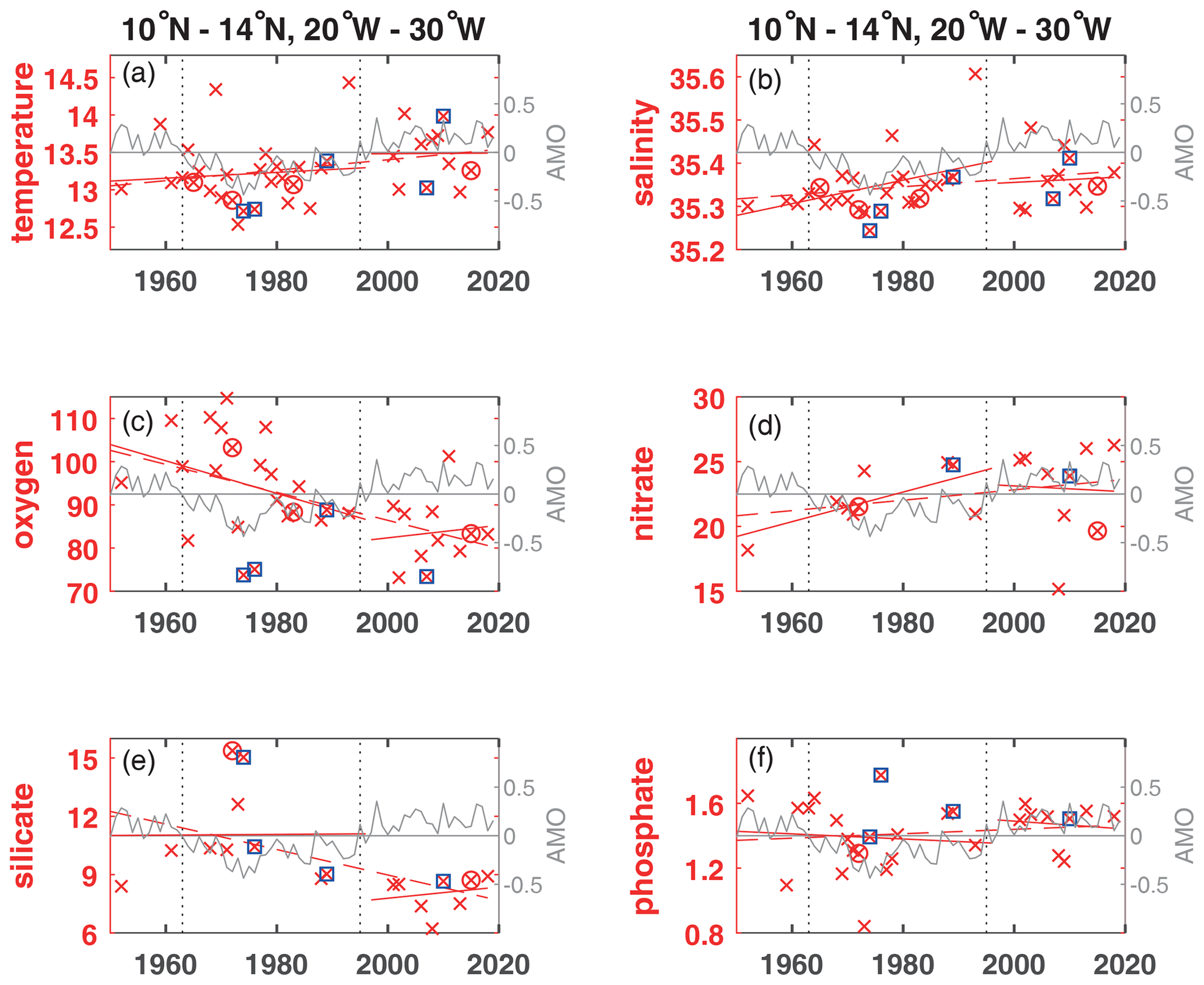
Figure 5Annual mean parameter concentration for years available (×) used to calculate trends for the layer 50 to 300 m plotted for the available years in the time period 1950 to 2018 (dashed red line) and for the positive and negative periods of the AMO in the Atlantic at area A for temperature (∘C) (a), salinity (b), oxygen (µmol kg−1) (c), nitrate (µmol kg−1) (d), silicate (µmol kg−1) (e) and phosphate (µmol kg−1) (f). The AMO is shown as a grey line. The change of AMO status in 1963 and 1995 is marked by dotted vertical lines. El Niño years defined as strong are marked by an additional magenta circle, and strong La Niña years are marked by an additional blue square.
In the 50 to 300 m layer of area A, despite the expected generally lower oxygen during positive AMO phase, oxygen increased in the positive AMO phase after 1995 (Fig. 3a), contrasting with the decrease in the 300 to 700 m layer (Fig. 2a). During the positive AMO phase after 1995 in the 50 to 300 m layer of area A, trends in temperature, oxygen, nitrate, silicate and phosphate (Fig. 5) changed sign compared to the long-term trend while salinity showed the same continuous trend as the positive long-term trend for this period. In contrast, none of these parameters changed during positive AMO compared to the long-term trend at the 50 to 300 m layer in the equatorial Atlantic in area B. In the tropical North Atlantic (area A) and the equatorial Atlantic (area B), the La Niña events showed lower than normal oxygen concentrations, especially for the years 1973/74, 1975/76 and 2010/11 (Fig. 3a, b). These years were not covered in the eastern tropical South Atlantic (area C). In the equatorial area B, the El Niño years 1965/66, 1972/73, 1987/88 and 1991/92 showed slightly higher than normal oxygen concentrations (Fig. 3b). Although not true for all ENSO events, there seems to be some influence of the La Niña and El Niño events in the eastern tropical and equatorial Atlantic, which might be due to the various types with different hydrographic impact of ENSO events described in literature.
In eastern Pacific regions near the Galapagos Islands (2–5∘ S, 84–87∘ W) and near the American continent in the CalCOFI region (34–35∘ N, 121–122∘ W) and the Peru region (7–12∘ S, 78–83∘ W), oxygen increased and nutrients decreased in the 50 to 300 m layer during the negative PDO phase before 1977, with opposing trends during the positive PDO phase after 1977 (Stramma et al., 2020). In contrast to the eastern Pacific, the eastern and central and equatorial areas D and E (Table 2) do not show the reversed trends in oxygen and nutrients; however, temperature and salinity indicate a reversal with the PDO phase, as the PDO index encapsulates the major mode of sea surface temperature variability in the Pacific. On a global scale, the long-term SST trend 1901–2012 was positive everywhere except for a region in the North Atlantic (IPCC 2013, Fig. 2.21). For 1981 to 2012, while the western Pacific showed a warming trend, a large region with decreasing SSTs was seen in the eastern and equatorial Pacific Ocean (IPCC 2013, Fig. 2.22). This agrees with the temperature reversal seen in areas D and E. However, if the time period after 1977 is looked at separately for the positive PDO phase 1977 to 1999 and the negative PDO phase 1999 to 2013 similar to that in the layer 300 to 700 m the layer 50 to 300 m also shows the expected high oxygen concentrations in the period 1977 to 1990 and lower oxygen concentrations during 1999 to 2010 (Fig. 3d, e).
Although ENSO is a signal originating in the Pacific, the equatorial Pacific areas D and E show no obvious oxygen concentration changes related to ENSO events (Fig. 3d, e). The central equatorial Pacific area E shows the highest mean 50 to 300 m temperature and oxygen concentrations and the lowest nitrate concentrations of all six areas investigated (Table 3). The low nitrate and phosphate and lower silicate compared to the eastern equatorial area D shows the nutrient concentration decreasing westward in the equatorial Pacific in the 50 to 300 m layer (Stramma et al., 2020; their Fig. 2). The principal source of nutrients to surface water is vertical flux by diffusion and advection and by regeneration (Levitus et al., 1993). At the sea surface airborne nutrient supply from land is contributed, and terrestrial runoff of fertilizer-derived nutrients and organic waste add nutrients to the ocean (Levin, 2018). The tongue of high nutrient concentrations at the equatorial Pacific compared to the subtropical Pacific results from upwelling near the American shelf (Levitus et al., 1993) and equatorial upwelling.
In the eastern Indian Ocean, as is the case in the 300 to 700 m layer, the temperature in the 50 to 300 m layer (Table 2) decreases and indicates other processes related to the oxygen decrease instead of warming. In the Indian Ocean the IOD shows large variability on shorter timescales. Observations indicate that positive IOD events prevent anoxia off the west coast of India (Vallivattathillan et al., 2017). The IOD is very variable with a slightly higher index after 1990. The few oxygen measurements in the 50 to 300 m layer indicate high mean oxygen concentrations in area F until 1990 with a decrease in oxygen and low oxygen concentrations with an increase in oxygen after 1990 (Fig. 3f). The higher oxygen concentrations before 1990 and lower oxygen concentrations afterwards are also visible in the 300 to 700 m layer (Fig. 2f). The ENSO events do not indicate a visible influence on the oxygen concentration in area F. The four La Niña events between 1988 and 2008 were either below or above the mean trend line; the same is true for the two El Niño events in 1973/74 and 1987/88 (Fig. 3f).
The time series expansion of the six areas in the tropical oceans to the 1950 to 2018 period showed a similar decrease in oxygen in the 300 to 700 m layer as described for the 1960 to 2008 period. Therefore, despite the overlying variability, the long-term deoxygenation in the tropical oceans is continuous for the 68-year period (Fig. S1). This confirms the indicated importance on the 48-year period (Stramma et al., 2008) of the oxygen trend for future oceanic scenarios. The salinity trends are weak and not statistically significant, except for a salinity increase of 0.0012 yr−1 in the 300 to 700 m layer of area A in the tropical Northeast Atlantic. A consistent pattern in vertical sections in the Pacific Ocean is that nitrate and phosphate increase with depth to about 500 m, with a slight maximum at intermediate depths of 500–1500 m, while silicate continues to increase with depth (Fiedler and Talley, 2006), which is clearly visible in the higher mean concentrations in the 300 to 700 m layer in comparison to the 50 to 300 m layer (Table 3).
The temperature trends were positive in the three Atlantic areas, but positive or negative in relation to the time period included in the Pacific Ocean and Indian Ocean areas. Hence, we can conclude that the decreasing oxygen is not fully coupled to the local temperature change. As the decline of oxygen in the tropical Pacific was not accompanied by a temperature increase, Ito et al. (2016) concluded that the cause of the oxygen decline must include changes in biological oxygen consumption and/or ocean circulation. Modeling the depth range 260 to 710 m depth range for the 1970s–1990s the region of areas D and E were mainly influenced by circulation variability (Ito et al., 2016).
Enhanced temperature differences between land and sea could intensify upwelling winds in eastern upwelling areas (Bakun, 1990). Observed and modeled changes in wind in the Atlantic and Pacific over the past 60 years appear to support the idea of increased upwelling winds (Sydeman et al., 2014). Coastal and equatorial upwelling enhance nutrients in the upper ocean; therefore, the increase of nutrients in the eastern and equatorial oceans might be caused by winds intensifying upwelling. More nutrients in the surface layer enhances production and subsequently export, and thus at greater depth its decay with increased respiration reduces the oxygen content. The sinking flux of organic matter, which over time depletes oxygen, while adding carbon and nutrients to subsurface waters, is known as the biological pump (Keeling et al., 2010) and could cause the often observed opposite trends in oxygen and nutrient trends in the 50 to 300 m layer investigated here. In the 50 to 300 m layer, oxygen, temperature, salinity and nutrients showed long-term trends that were different in the three ocean basins. Nitrate increased in all areas. Phosphate also increased in the Atlantic Ocean and Indian Ocean areas, while it decreased in the two areas of the equatorial Pacific Ocean. The phosphate increase in the Atlantic Ocean might be related to a continuous phosphate supply with the Saharan dust distributed over the Atlantic Ocean with the wind (Gross et al., 2015). Silicate decreased in the Atlantic and Pacific areas but increased in the eastern Indian Ocean. Often the expected inverse trend of oxygen and nutrients caused by remineralization of marine detritus (Whitney et al., 2013) was observed; however, variations based on other drivers influence the nutrient trends.
To summarize the results for the different Ocean basins in the Atlantic Ocean, oxygen decreases and temperature and salinity increase for both depth layers, except in the eastern tropical South Atlantic (area C) for the 50 to 300 m layer, where oxygen slightly increases in the Angola Dome region. In the Pacific Ocean and Indian Ocean oxygen decreases; however, temperature and salinity either increase or decrease. The trends for nutrients are often not in the 95 % confidence range but indicate a nitrate and phosphate increase with a silicate decrease in the Atlantic and a nitrate increase and phosphate and silicate decrease in the Pacific, while in the eastern tropical Indian Ocean nitrate, silicate and phosphate increase. Nutrient variability indicates that their trends are more dependent on local drivers in addition to a global trend.
An influence of ENSO years on the oxygen distribution with lower mean oxygen concentrations in the 50 to 300 m layer in La Niña years and larger oxygen concentrations in El Niño years was visible in the tropical North Atlantic and equatorial Atlantic. No clear impact of ENSO was observed in the tropical South Atlantic and the Pacific Ocean and Indian Ocean areas (C to F).
To construct time series in areas with low data availability measurements from larger areas had to be taken into account. As a result, there is a possible bias due to the distribution of the measurements within the area and due to gaps in the time line. In addition, there might be variations due to the measurement techniques for oxygen and nutrients and the use of different reference material for nutrient measurements or applied bias for nutrient measurements. Utilization of historical nutrient data to assess decadal trends has been hindered by their inaccuracy, manifested as offsets in deep-water concentrations measured by different laboratories (Zhang et al., 2000). Although the trends are often not 95 % significant, the results indicate existing trends and climate-related changes. As a consequence, there is the possibility of a larger variability in the computed trends compared to the earlier investigation of these areas in Stramma et al. (2008). Later measurements reported in the literature confirmed the described decrease in oxygen (Stramma et al., 2008) in the tropical oceans (e.g., Hahn et al., 2017). The not statistically significant trends described here might be verified with additional data in the future, especially in cases where the drift observed in float measurements can be removed and float data be added to extend the data sets. Changing the depth layer of the trend computations leads to different mean parameter values (Table 3) and may result in some minor variations in the trend computation. However, as the oxygen trends for the 50 to 300 m layer and the 300 to 700 m layer are all negative (except for the 50 to 300 m layer of area C due to a local effect) the result of oxygen decrease is not related to the depth layer chosen.
Although the database is small, especially for nutrients, there is an indication that variability overlain on the long-term trends is connected to climate modes, as was found in the eastern Pacific with reversing trends related to the PDO (Stramma et al., 2020). The six areas of the tropical ocean basins indicate some connection to the climate modes of the three ocean basins. In the tropical eastern North Atlantic (area A), there is some dependence with the AMO. In areas D and E in the equatorial Pacific, a connection to the PDO is visible when the positive PDO phase 1977 to 1999 and the negative PDO phase 1999 to 2013 are looked at separately. In the eastern tropical Indian Ocean there seems to be some dependence to the state of the IOD, despite the fact that the IOD varies more on shorter timescales and that the IOD change in 1990 is weak.
Future measurements of temperature, salinity, oxygen and nutrients could lead to more stable results when determining trends and their variability to better understand the influence of climate change on the ocean ecosystem and prepare future predictions of ocean oxygen from Earth system models (Frölicher et al., 2016). Making existing nutrient data that are so far not in public databases available to the public and modeling efforts on oxygen and nutrient changes would further improve the understanding of oxygen and nutrient variability and its biological influence, e.g., on fisheries. The first ecosystem changes like habitat compression can be observed, and negative impacts are expected on biological regulation, nutrient cycling and fertility, and sea food availability, with an increasing risk of fundamental and irreversible ecological transformations (Hoegh-Guldberg and Bruno, 2010). The implication of oxygen trends for biology and successive human impacts is quite large, and a lot of literature supports this. All aspects of oxygen trends are discussed in the different chapters of the IUCN report (Laffoley and Baxter, 2019).
The AMO time series was taken from https://www.esrl.noaa.gov/psd/data/timeseries/AMO/ (ESRL, Climate time series, last access: 17 February 2020). The Indian Ocean Dipole Mode was taken from https://www.esrl.noaa.gov/psd/gcos_wgsp/Timeseries/Data/dmi.long.data (last access: 3 March 2020). The yearly PDO data were taken from http://ds.data.jma.go.jp/tcc/tcc/products/elnino/decadal/annpdo.txt (last access: 9 July 2020) from the Japan Meteorological Society covering the period 1901 to 2019.
The bottle data from cruises in 2016 at 170∘ W (096U2016426_hyd1.csv) and at 110∘ W (33RO20161119_hyd1.csv) were downloaded from the CCHDO at the University of California San Diego (https://cchdo.ucsd.edu, CCHDO, 2020, last access: 8 November 2018).
The added ship cruises provided the CTD data in the data sets for RV Meteor cruise M119 (Schmidtko, 2021), for RV Meteor cruises M120 https://doi.pangaea.de/10.1594/PANGAEA.868654 (Kopte and Dengler, 2016), M130 https://doi.pangaea.de/10.1594/PANGAEA.903913 (Burmeister et al., 2019), M131 https://doi.pangaea.de/10.1594/PANGAEA.910994 (Brandt et al., 2020), M145 https://doi.pangaea.de/10.1594/PANGAEA.904382 (Brandt and Krahmann, 2019), and M148 (Schmidtko, 2021) and RV Merian MSM07 (Schmidtko, 2021), and nutrient data were provided from the data sets of RV Merian MSM10/1 https://doi.pangaea.de/10.1594/PANGAEA.775074 (Tanhua et al., 2012); RV Poseidon 250 (Schmidtko, 2021), M68/2 https://www.ncei.noaa.gov/data/oceans/ncei/ocads/data/0108078/, M83/1 https://doi.pangaea.de/10.1594/PANGAEA.821729 (Tanhua, 2013), and M97 https://doi.pangaea.de/10.1594/PANGAEA.863119 (Tanhua, 2016); and M106 (Schmidtko, 2021), M119 (Schmidtko, 2021), M130 https://doi.pangaea.de/10.1594/PANGAEA.913986 (Tanhua, 2020), M131 (Schmidtko, 2021), M145 (Schmidtko, 2021), and M148 (Schmidtko, 2021).
The supplement related to this article is available online at: https://doi.org/10.5194/os-17-833-2021-supplement.
LS conceived the study and wrote the manuscript. SuS compiled the data for the time series, collected further references, and discussed and modified the manuscript.
The authors declare that they have no conflict of interest.
Support was received through GEOMAR and the Deutsche Forschungsgemeinschaft (DFG) as part of the “Sonderforschungsbereich 754: Climate–Biogeochemistry Interactions in the Tropical Ocean”.
This research has been supported by the Deutsche Forschungsgemeinschaft (grant no. SFB754).
The article processing charges for this open-access publication were covered by the GEOMAR Helmholtz Centre for Ocean Research Kiel.
This paper was edited by Arvind Singh and reviewed by Karen Wishner and two anonymous referees.
Allison, E. H. and Bassett, H. R.: Climate change in the oceans: Human impacts and responses, Science, 350, 778–782, https://doi.org/10.1126/science.aac8721, 2015.
Ayers, J. M., Strutton, P. G., Coles, V. J., Hood, R. R., and Matear, R. J.: Indonesian throughflow nutrient fluxes and their potential impact on Indian Ocean productivity, Geophys. Res. Lett., 41, 5060–5067, https://doi.org/10.1002/2014GL060593, 2014.
Bakun, A.: Global climate change and the intensification of coastal upwelling, Science, 247, 198–201, 1990.
Bastin, S., Claus, M., Brandt, P., and Greatbatch, R. J.: Equatorial deep jets and their influence on the mean equatorial circulation in an idealized ocean model forced by intraseasonal momentum flux convergence, Geophys. Res. Lett., 47, e2020GL087808, https://doi.org/10.1029/2020GL087808, 2020.
Bograd, S. J., Pozo Buil, M., Di Lorenzo, E., Castro, C. G., Schroeder, I. D., Goericke, R., Anderson, C. R., Benitez-Nelson, C., and Whitney, F. A.: Changes in source waters to the Southern California Bight, Deep-Sea Res. Pt. II, 112, 42–52, https://doi.org/10.1016/j.dsr2.2014.04.009, 2015.
Brandt, P. and Krahmann, G.: Physical Oceanography (CTD) during METEOR cruise M145, PANGAEA, https://doi.org/10.1594/PANGAEA.904382, 2019.
Brandt, P., Kopte, R., and Krahmann, G.: Physical oceanography (CTD) during METEOR cruise M131, PANGAEA, https://doi.org/10.1594/PANGAEA.910994, 2020.
Bretherton, F. P., Davis, R. E., and Fandry, C. B.: A technique for objective analysis and design of oceanographic experiments applied to MODE-73, Deep-Sea Res., 23, 559–582, https://doi.org/10.1016/0011-7471(76)90001-2, 1976.
Burmeister, K., Lübbecke, J., Brandt, P., Claus, M., and Hahn, J.: Ventilation of the eastern tropical North Atlantic by intraseasonal flow events of the North Equatorial Undercurrent, PANGAEA, https://doi.org/10.1594/PANGAEA.903913, 2019.
CCHDO: Welcome to the CCHDO, available at: https://cchdo.ucsd.edu, last access: 13 February 2020.
Cheung, W. W. L., Sarmiento, J. L., Dunne, J., Frölicher, T. L., Lam, V. W. Y., Palomares, M. L. D., Watson, R., and Pauly, D.: Shrinking of fishes exacerbates impacts of global ocean changes of marine ecosystems, Nat. Clim. Change, 3, 254–258, https://doi.org/10.1038/nclimate1691, 2013.
Deser, C., Alexander, M. A., Xie, S.-P., and Phillips, A. S.: Sea surface temperature variability: Patterns and mechanisms, Annu. Rev. Mar. Sci., 2, 115–143, https://doi.org/10.1146/annurev-marine-120408-151453, 2010. Annu. Rev. Mar. Sci. 2, 115-143
Deutsch, C., Brix, H., Ito, T., Frenzel, H., and Thompson, L.: Climate-forced variability of ocean hypoxia, Science, 333, 336–339, https://doi.org/10.1126/science.1202422, 2011.
Fiedler, P. C. and Talley, L. D.: Hydrography of the eastern tropical Pacific: A review, Prog. Oceanogr., 69, 143–180, 2006.
Frölicher, T. L., Rogers, K. B., Stock, C. A., and Cheung, W. L. W.: Sources of uncertainties in 21th century projections of potential ecosystem stressors, Global Biogeochem. Cy., 30, 1224–1243, https://doi.org/10.1002/2015GB005338, 2016.
Gilly, W. F., Beman, J. M., Litvin, S. Y., and Robinson, B. H.: Oceanographic and biological effects of shoaling of the oxygen minimum zone, Annu. Rev. Mar. Sci., 5, 393–420, https://doi.org/10.1146/annurev-marine-120710-100849, 2013.
Gouretski, V. V. and Jancke, K.: Systematic errors as the cause for an apparent deep water property variability: Global analysis of the WOCE and historical hydrographic data, Prog. Oceanogr., 48, 337–402, 2001.
Gross, A., Goren, T., Pio, C., Cardoso, J., Tirosh, O., Todd, M. C., Rosenfeld, D., Weiner, T., Custódio, D., and Angert, A.: Variability in Sources and Concentrations of Saharan Dust Phosphorus over the Atlantic Ocean, Environ. Sci. Tech. Let., 2, 31–37, 2015.
Hahn, J., Brandt, P., Schmidtko, S., and Krahmann, G.: Decadal oxygen change in the eastern tropical North Atlantic, Ocean Sci., 13, 551–576, https://doi.org/10.5194/os-13-551-2017, 2017.
Ham, Y., Choi, J., and Kug, J.: The weakening of the ENSO-Indian Ocean Dipole (IOD) coupling strength in recent decades, Clim. Dynam., 49, 249–261, https://doi.org/10.1007/s00382-016-3339-5, 2017.
Hoegh-Guldberg, O. and Bruno, J. F.: The impact of climate change on the world's marine ecosystems, Science, 328, 1523–1528, https://doi.org/10.1126/science.1189930, 2010.
Hurrell, J. W. and Deser, C.: North Atlantic climate variability: The role of the North Atlantic Oscillation, J. Marine Syst., 79, 231–244, https://doi.org/10.1016/j.jmarsys.2009.11.002, 2010.
IPCC: Climate Change 2013: The Physical Science Basis, in: Contribution of Working Group I to the Fifth Assessment Report of the Intergovernmental Panel on Climate Change, edited by: Stocker, T. F., Qin, D., Plattner, G.-K., Tignor, M., Allen, S. K., Boschung, J., Nauels, A., Xia, Y., Bex, V., and Midgley, P. M., Cambridge University Press, Cambridge, United Kingdom, New York, USA, 1535 pp., 2013.
Ito, T., Nenes, A., Johnson, M. S., Meskhidze, N., and Deutsch, C.: Acceleration of oxygen decline in the tropical Pacific over the past decades by aerosol pollutants, Nat. Geosci., 9, 443–448, https://doi.org/10.1038/NGEO2717, 2016.
Ito, T., Minobe, S., Long, M. C., and Deutsch, C.: Upper ocean O2 trends: 1958–2015, Geophys. Res. Lett., 44, 4214–4223, https://doi.org/10.1002/2017GL073613, 2017.
Johnson, G. C., Robbins, P. E., and Hufford, G. E.: Systematic adjustments of hydrographic sections for internal consistency, J. Atmos. Ocean. Tech., 18, 1234–1244, https://doi.org/10.1175/1520-0426(2001)018<1234:SAOHSF>2.0.CO;2, 2001.
Keeling, R. F., Körtzinger, A., and Gruber, N.: Ocean deoxygenation in a warming world, Annu. Rev. Mar. Sci., 2, 199–229, 2010.
Kopte, R. and Dengler, M.: Physical oceanography during METEOR cruise M120, PANGAEA, https://doi.org/10.1594/PANGAEA.868654, 2016.
Laffoley, D. and Baxter, J. M. (Eds.): Ocean deoxygenation: Everyone's problem – Causes, impacts, consequences and solutions, Full report, IUCN, Gland, Switzerland, 580 pp., https://doi.org/10.2305/IUCN.ch.2019.13.en, 2019.
Latif, M. and Grötzner, A.: The equatorial Atlantic oscillation and its response to ENSO, Clim. Dynam., 16, 213–218, https://doi.org/10.1007/s003820050014, 2000.
Levin, L. A.: Manifestation, drivers, and emergence of open ocean deoxygenation, Annu. Rev. Mar. Sci., 10, 229–260, https://doi.org/10.1146/annurev-marine-12916-063359, 2018.
Levitus, S., Conkright, M. E., Reid, J. L., Najjar, R. G., and Mantyla, A.: Distribution of nitrate, phosphate and silicate in the world oceans, Prog. Oceanogr., 31, 254–273, 1993.
Li, G., Cheng, L., Zhu, J., Trenberth, K. E., Mann, M. E., and Abraham, J. P.: Increasing ocean stratification over the past half-century, Nat. Clim. Change, 10, 1116–1123, https://doi.org/10.1038/s41558-020-00918-2, 2020.
Louanchi, F. and Najjar, R. G.: A global monthly climatology of phosphate, nitrate, and silicate in the upper ocean: Spring-summer export production and shallow remineralization, Global Biogeochem. Cy., 14, 957–977, 2000.
Mazeika, P. A.: Thermal domes in the eastern tropical Atlantic Ocean, Limnol. Oceanogr., 12, 537–539, 1967.
McPhaden, M. J., Zebiak, S. E., and Glantz, M. H.: ENSO as an Integrating Concept in Earth Science, Science, 314, 1740–1745, https://doi.org/10.1126/science.1132588, 2006.
Montes, E., Muller-Karger, F. E., Cianca, A., Lomas, M. W., and Habtes, S.: Decadal variability in the oxygen inventory of North Atlantic subtropical underwater captured by sustained, long-term oceanographic time series, Global Biogeochem. Cy., 30, 460–478, https://doi.org/10.1002/2015GB005183, 2016.
Nicholson, S. E.: An analysis of the ENSO signal in the tropical Atlantic and western Indian Oceans, Int. J. Climatol., 17, 345–375, https://doi.org/10.1002/(SICI)1097-0088(19970330)17:4<345::AID-JOC127>3.0.CO;2-3, 1997.
Ono, T., Shiomoto, A., and Saino, T.: Recent decrease of summer nutrients concentrations and future possible shrinkage of the subarctic North Pacific high-nutrient low-chlorophyll region, Global Biogeochem. Cy., 22, GB3027, https://doi.org/10.1029/2007GB003092, 2008.
Oschlies, A.: NAO-induced long-term changes in nutrient supply to the surface waters of the North Atlantic, Geophys. Res. Lett., 28, 1751–1754, https://doi.org/10.1029/2000GL012328, 2001.
Palter, J. B., Lozier, M. S., and Barber, R. T.: The effect of advection on the nutrient reservoir in the North Atlantic subtropical gyre, Nature, 437, 687–692, 2005.
Saji, N. N., Goswami, B. N., Vinayachandran, P. N., and Yamagata, T.: A dipole mode in the tropical Indian Ocean, Nature, 401, 360–363, https://doi.org/10.1038/43854, 1999.
Schmidtko, S.: data_collection_Stramma_Schmidtko_Ocean_ Sci_2021.zip, available at: https://cloud.geomar.de/s/tmJWCFJ27gPBmpa, last access: 29 June 2021.
Schmidtko, S., Johnson, G. C., and Lyman, J. M.: MIMOC: A global monthly isopycnal upper-ocean climatology with mixed layers, J. Geophys. Res.-Oceans, 118, 1658–1672, https://doi.org/10.1002/jgrc.20122, 2013.
Schmidtko, S., Stramma, L., and Visbeck, M.: Decline in global oceanic oxygen content during the past five decades, Nature, 542, 335–339, https://doi.org/10.1038/nature21399, 2017.
Shepherd, J. G., Brewer, P. G., Oschlies, A., and Watson, A. J.: Ocean ventilation and deoxygenation in a warming world: introduction and overview, Philos. T. Roy. Soc. A, 375, 20170240, https://doi.org/10.1098/rsta.2017.0240, 2017.
Sigman, D. M. and Hain, M. P.: The biological productivity of the ocean, Nature Education, 3, 1–16, 2012.
Stramma, L., Johnson, G. C., Sprintall, J., and Mohrholz, V.: Expanding Oxygen-Minimum Zones in the Tropical Oceans, Science, 320, 655–658, https://doi.org/10.1126/science.1153847, 2008.
Stramma, L., Prince, E. D., Schmidtko, S., Luo, J., Hoolihan, J. P., Visbeck, M., Wallace, D. W. R., Brandt, P., and Körtzinger, A.: Expansion of oxygen minimum zones may reduce available habitat for tropical pelagic fishes, Nat. Clim. Change, 2, 33–37, https://doi.org/10.1038/nclimate1304, 2012.
Stramma, L., Schmidtko, S., Bograd, S. J., Ono, T., Ross, T., Sasano, D., and Whitney, F. A.: Trends and decadal oscillations of oxygen and nutrients at 50 to 300 m depth in the equatorial and North Pacific, Biogeosciences, 17, 813–831, https://doi.org/10.5194/bg-17-813-2020, 2020.
Sydeman, W. J., García-Reyes, M., Schoeman, D. S., Rykaczewski, R. R., Thompson, S. A., Black, B. A., and Bograd, S. J.: Climate change and wind intensification in coastal upwelling ecosystems, Science, 345, 77–80, 2014.
Tanhua, T.: Hydrochemistry of water samples during METEOR cruise M83/1, PANGAEA, https://doi.org/10.1594/PANGAEA.821729, 2013.
Tanhua, T.: Hydrochemistry of water samples during METEOR cruise M97, PANGAEA, https://doi.org/10.1594/PANGAEA.863119, 2016.
Tanhua, T., van Heuven, S., Key, R. M., Velo, A., Olsen, A., and Schirnick, C.: Quality control procedures and methods of the CARINA database, Earth Syst. Sci. Data, 2, 35–49, https://doi.org/10.5194/essd-2-35-2010, 2010.
Tanhua, T., Stramma, L., Desai, F., and Löscher, C. R.: Hydrochemistry and molecular biology during Maria S. Merian cruise MSM10/1, IFM-GEOMAR Leibniz-Institute of Marine Sciences, Kiel University, Kiel, Germany, PANGAEA, https://doi.org/10.1594/PANGAEA.775074, 2012.
Vallivattathillam, P., Iyyappan, S., Lengaigne, M., Ethé, C., Vialard, J., Levy, M., Suresh, N., Aumont, O., Resplandy, L., Naik, H., and Naqvi, W.: Positive Indian Ocean Dipole events prevent anoxia off the west coast of India, Biogeosciences, 14, 1541–1559, https://doi.org/10.5194/bg-14-1541-2017, 2017.
Whitney, F. A., Bograd, S. J., and Ono, T.: Nutrient enrichment of the subarctic Pacific Ocean pycnocline, Geophys. Res. Lett., 40, 2200–2205, https://doi.org/10.1002/grl.50439, 2013.
Williams, R. G. and Follows, M. J.: Physical transport of nutrients and the maintenance of biological production, in: Ocean Biogeochemistry: Global Change, The IGBP Series, edited by: Fasham, M. J. R., Springer, Berlin, Heidelberg, Germany, 2003.
Wishner, K. F., Outram, D. M., Seibel, B. A., Daly, K. L., and Williams, R. L.: Zooplankton in the eastern tropical North Pacific: Boundary effects of oxygen minimum zone expansion, Deep-Sea Res. Pt. I, 79, 122–140, https://doi.org/10.1016/j.dsr.2013.05.012, 2013.
Zhang, J.-Z., Mordy, C. W., Gordon, L. I., Ross, A., and Garcia, H. E.: Temporal trends in deep ocean Redfield ratios, Science, 289, 1839a, https://doi.org/10.1126/science.289.5486.1839a, 2000.