Spatiotemporal structure of Baltic free sea level oscillations in barotropic and baroclinic conditions from hydrodynamic modelling

Free sea level oscillations in barotropic and baroclinic conditions were examined using numerical experiments based on a 3-D hydrodynamic model of the Baltic Sea. In a barotropic environment, the highest amplitudes of free sea level oscillations are observed in the northern Gulf of Bothnia, eastern Gulf of Finland, and south-western Baltic Sea. In these areas, the maximum variance appears within the frequency range corresponding to periods of 13–44 h. In a stratified environment, after the cessation of meteorological forcing, water masses relax to the equilibrium state in the form of mesoscale oscillations at the same frequencies as well as in the form of rapidly decaying low-frequency (seasonal) oscillations. The total amplitudes of free baroclinic perturbations are significantly larger than those of barotropic perturbations, reaching 15–17 cm. Contrary to barotropic, oscillations in baroclinic conditions are strongly pronounced in the deep-water areas of the Baltic Sea proper. Specific spatial patterns of amplitudes and phases of free barotropic and baroclinic sea level oscillations identified them as progressive–standing waves representing barotropic or baroclinic modes of gravity waves and topographic Rossby waves.

1 Introduction

The Baltic Sea level perturbations represent a superposition of free and forced oscillations of different spatial and temporal scales. These oscillations can be generated either within the Baltic basin or come from the North Sea via the narrow and shallow Danish straits (Samuelsson and Stigebrandt, 1996). The Baltic Sea water masses experience the continuous effect of external and internal forces related to tides, wind stress, atmospheric pressure, and changes of water density or of water balance constituents. After cessation of the perturbing forces, the water masses return to equilibrium in the form of barotropic or baroclinic modes of free oscillations, rapidly attenuated by dissipative forces (Leppäranta and Myrberg, 2009; Proshutinsky, 1993; Zakharchuk et al., 2004).

Free sea level oscillations are directly related to the eigenoscillations of sea basins. The spectral structure of eigenoscillations depends on sea basin scales, basin bathymetry, and land configuration. In eigenoscillation frequencies, the basin water masses return to equilibrium conditions after meteorological forcing (Fennel and Seifert, 2008; Leppäranta and Myrberg, 2009; Lisitzin, 1974). Within these frequencies, the free oscillations may resonate with wind forcing, resulting in an anomalous sea level rise followed by the inundation of coastal areas (Jönsson et al., 2008; Zakharchuk and Tikhonova, 2011). The investigation into free oscillations of sea basins is essential for correctly interpreting the spatiotemporal variability of physical, hydrochemical, and biological parameters, as well as for identifying the mechanisms responsible for this variability.

The Baltic Sea free oscillations are usually related to seiches. Seiches are free sea level fluctuations in an enclosed or semi-isolated basin, which occur as standing waves generated by external forcing and continue due to inertia after cessation of the initial force (Lisitzin, 1959; Proudman, 1953; Pugh, 1987). Previous studies based on spectral analysis of the Baltic Sea tide gauge records have described several Baltic seiche systems. One system is located on the western Baltic–Gulf of Finland axis and is characterised by periods of 26–32 h in the primary mode and 17–20 h in the secondary mode (Kulikov and Medvedev, 2013; Lisitzin, 1959; Magaard and Krauss, 1966; Neumann, 1941). The primary mode of the second rapidly damping seiche system, situated in the western Baltic–Bay of Bothnia axis, has a 39 h period (Neumann, 1941).

Using a one-dimensional simplified numeric model, on the axis the Gulf of Finland–Danish straits, Neumann (1941) detected seiches with a 27 h period. The amplitude of these seiches was usually less than 10 cm, rarely reaching 40 cm. Nevertheless, higher amplitudes were not excluded.

Metzner et al. (2000) demonstrated that the Baltic free sea level oscillations can be studied using satellite altimetry combined with numerical modelling and in situ observations.

Research on free sea level oscillations based on numerical modelling found a more complex system of seiches in the Baltic Sea. Using a two-dimensional shallow-water model with 10 km spatial resolution, Wübber and Krauss (1979) suggested 10 modes of Baltic Sea eigenoscillations. The first four modes have periods of 31, 26, 22, and 20 h, respectively. The authors noted that the eigenoscillations were significantly modified by the Coriolis force. Earth's rotation transforms all modes of eigenoscillations to positive amphidromic waves. As a result, the period of oscillations may diminish (if this period is higher than an inertial period) or may increase (if it is lower than the inertial period).

Subsequently, Jönsson et al. (2008), based on the analysis of linear shallow-water model simulations, identified three different local oscillatory modes: in the Gulf of Finland (with two 23 and 27 h periods), Danish Great Belt (with periods of 23–27 h), and Gulf of Riga (with 17 h periods). The authors attributed these variations to seiches and noted that they were not connected to each other. However, this conclusion is not convincing, as it was not supported by the spatiotemporal distribution of the oscillation phases. The authors also suggested that the Baltic free sea level oscillations can be related to Kelvin waves that propagate from the Gulf of Finland into the Baltic Proper along the coastline.

Another study (Zakharchuk et al., 2004) that was based on simulation results of a hydrodynamic three-dimensional model implies that low-frequency free oscillations in the Baltic Sea represent the topographic Rossby waves because their phase velocity is significantly lower than that of the barotropic gravity waves.

All previous studies based on numerical modelling investigated only the barotropic variations in the Baltic sea level, while an actual sea basin is a baroclinic system. The specifics of the relaxation of the Baltic Sea water masses to equilibrium after the cessation of meteorological forces in baroclinic conditions remain unclear.

The present study investigates the difference between barotropic and baroclinic free sea level oscillations in the Baltic Sea using a three-dimensional hydrodynamic model. First, the capability of the model to simulate sea level fluctuations in different parts of the Baltic Sea was verified against in situ tide gauge observations (Sect. 2.3). Then, the spatiotemporal structure of the sea level variations in barotropic (Sect. 3.1) and baroclinic (Sect. 3.2) conditions is analysed using Fourier analyses of the model outputs. To interpret the detected free sea level oscillations, we compared the estimated phase speed of the modelled oscillations with the theoretical phase speed values of barotropic and baroclinic gravity waves and discuss the results in Sect. 4.

2 Data and methods

A three-dimensional non-linear baroclinic model developed by the Institute of Numerical Mathematics of the Russian Academy of Science (Institute of Numerical Mathematics Ocean Model or INMOM) was selected for studying the Baltic free sea level oscillations (Diansky et al., 2006; Zalesny et al., 2012). The model was configured for the Baltic Sea basin and run in its basic setup to ensure the credibility of the sea level simulations. Then, the model was reconfigured for two numerical experiments to represent the barotropic and baroclinic conditions in the Baltic Sea.

2.1 Model description

INMOM is based on primitive equations of ocean hydrodynamics in spherical coordinates and on hydrostatic and Boussinesq approximations. A dimensionless value σ is used as the vertical coordinate, which is specified as $\mathit{\sigma }=(z-\mathit{\zeta })/(H-\mathit{\zeta })$, where z is the vertical coordinate; $\mathit{\zeta }=\mathit{\zeta }(\mathit{\lambda },\mathit{\phi },t)$ is the deviation of the sea surface height (SSH) from the undisturbed surface as a function of longitude λ, latitude ϕ, and time t; and $H=H(\mathit{\lambda },\mathit{\phi })$ is the sea depth (Diansky, 2013). The prognostic variables of the model are the horizontal components of the velocity vector, potential temperature T, salinity S, and deviation of sea surface height from undisturbed surface. The equation of state specially designed for the numerical models is used to calculate the water density (Brydon et al., 1999).

INMOM includes a sea ice module that takes into account the dynamics of the sea ice, ice melting, and formation of sea ice and snow, as well as the transformation of old snow to sea ice (Yakovlev, 2009). This module calculates the ice drift velocity, which depends on wind, sea currents, Earth's rotation, sea surface slope, and ice floe interactions described by elastic–viscous–plastic rheology (Briegleb et al., 2004). The ice module uses a monotonic transfer scheme (Hunke and Dukowicz, 1997), ensuring non-negative values of ice/snow concentrations and mass. A detailed description of the basic configuration of INMOM can be found in Moshonkin et al. (2018).

INMOM has been widely used in studies of the Black and Azov seas (Fomin and Diansky, 2018; Korshenko et al., 2019; Zalesny et al., 2012), the Norwegian Sea (Morozov et al., 2019), the Barents Sea (Diansky et al., 2019), and the Sea of Okhotsk (Diansky et al., 2020). For this study, INMOM was run for 2 years (2009–2010) within the region bounds of 53.6–65.9^∘ N and 9.4–30.4^∘ E, with a spatial resolution of 2 nautical miles (3.7 km) in the horizontal direction, non-uniform 35σ levels in the vertical direction, and a 2.5 min calculation step. The model outputs represent the 6 h averaged sea level height.

The Baltic Sea bottom topography was downloaded from the Baltic Nest Institute portal (http://nest.su.se, last access: 5 April 2021). The initial bathymetric product of 1^′ × 1^′ resolution was recalculated to match the 2-mile resolution of the model grid. On the solid boundaries, no-normal flow and free-slip boundary conditions for momentum were applied, and the heat and salt fluxes were set to zero.

The mean monthly water temperature and salinity fields provided by the Copernicus Marine Service Information portal (http://marine.copernicus.eu, last access: 5 April 2021) were used for model initialisation. This product represents the output of the three-dimensional High Resolution Model for the Baltic Sea – Baltic Operational Oceanography System (HIROMB-BOOS or HBM-V1) baroclinic hydrodynamic ocean model, assimilating the in situ vessel and satellite observations. The data cover the 1990–2009 period and contain the sea level, current velocity, temperature, and salinity with a 5.6 km horizontal and 5 m vertical resolution.

INMOM was forced using ERA-Interim atmospheric reanalysis (Berrisford et al., 2011). The reanalysis has a 0.75^∘ spatial resolution and 6 h temporal resolution. INMOM used the following forcing parameters: air temperature and humidity at an altitude of 2 m, atmospheric pressure at sea level, wind speed of 10 m, precipitation, and short-wave and long-wave radiation.

The liquid boundary was drawn in the Kattegat Strait along 57.73^∘ N (Fig. 1) and defined using the Copernicus mean monthly values of sea temperature and salinity, as well as the hourly sea level records on two tide gauge stations, Frederikshavn (57.43^∘ N, 10.57^∘ E) and Gothenburg Torshamnen (57.68^∘ N, 11.79^∘ E), located on the east and west coasts of the strait, respectively. In situ sea level measurements from these stations were interpolated to the model grid nodes along the liquid boundary line.

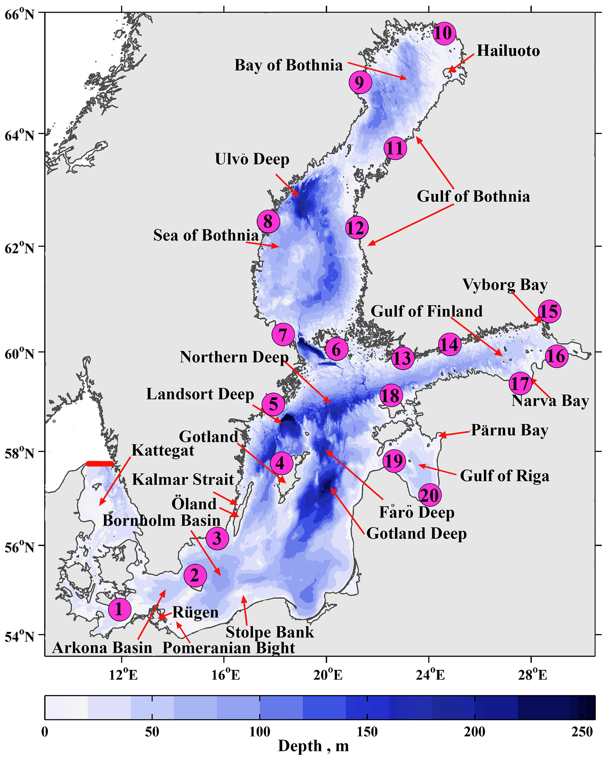
Figure 1 Bathymetry and locations of tide gauge stations used for model validation. The liquid boundary of the modelled area in the Kattegat Strait is indicated by bold red line. The map is created using the Baltic Sea Bathymetry Database (BSBD) http://data.bshc.pro/ (last access: 5 April 2021).

Water level observations at 20 other gauging stations (Fig. 1) served to validate the model outputs. In situ data were provided by the Copernicus Marine Service and the Northwest Hydrometeorological Service of Russia. Table 1 presents the metadata of the stations used for validation. The in situ time series are sufficient for the validation exercise and have only a few gaps. The percentage of missing data (found only for six stations) does not exceed 6.1 %. For the validation procedure, the in situ observations were averaged to match the 6 h output frequency of the model.

Table 1 Tide gauge stations used in the study (state for study period 2009–2010).

2.2 Model validation

The sea level simulated by the basic INMOM configuration was verified against the in situ observations using a set of standard statistical parameters: absolute (σ_abs) and relative (σ_rel) bias, root mean square error (σ_er), and correlation coefficient (R). The standard deviations of the observed (σ_tg) and simulated (σ_m) sea surface heights, as well as their ratio (σ_p), were evaluated, and the additional parameter of accuracy (P_m, %) was introduced. The P_m parameter allows the assessment of the number of good simulations (compared to total number of outputs) considering their accuracy <0.674σ_tg.

$$\begin{array}{}\text{(1)}& {\mathit{\sigma }}_{\mathrm{abs}}={\displaystyle \frac{\sum _{i=\mathrm{1}}^N\left|{\mathit{\zeta }}_{\mathrm{m}}-{\mathit{\zeta }}_{\mathrm{tg}}\right|}{N}},\end{array}$$

where N is the time series length, ζ_m is the modelled sea level, and ζ_tg is the tide gauge observations.

$$\begin{array}{}\text{(2)}& {\mathit{\sigma }}_{\mathrm{rel}}={\displaystyle \frac{{\mathit{\sigma }}_{\mathrm{abs}}\cdot \mathrm{100}\mathit{\%}}{({\mathit{\zeta }}_{\mathrm{tg}}{)}_{max}-({\mathit{\zeta }}_{\mathrm{tg}}{)}_{min}}},\end{array}$$

where (ζ_tg)_max is the maximum and (ζ_tg)_min is the minimum value of the in situ observations.

$$\begin{array}{}\text{(3)}& {\displaystyle }{\mathit{\sigma }}_p={\displaystyle \frac{{\mathit{\sigma }}_{\mathrm{er}}\cdot \mathrm{100}\mathit{\%}}{{\mathit{\sigma }}_{\mathrm{tg}}}},\text{(4)}& {\displaystyle }R={\displaystyle \frac{\frac{\mathrm{1}}{N-\mathrm{1}}\sum _{i=\mathrm{1}}^N({\mathit{\zeta }}_{\mathrm{tg}}-\stackrel{\mathrm{‾}}{{\mathit{\zeta }}_{\mathrm{tg}}})({\mathit{\zeta }}_{\mathrm{m}}-\stackrel{\mathrm{‾}}{{\mathit{\zeta }}_{\mathrm{m}}})}{{\mathit{\sigma }}_{\mathrm{tg}}{\mathit{\sigma }}_m}}\end{array}$$

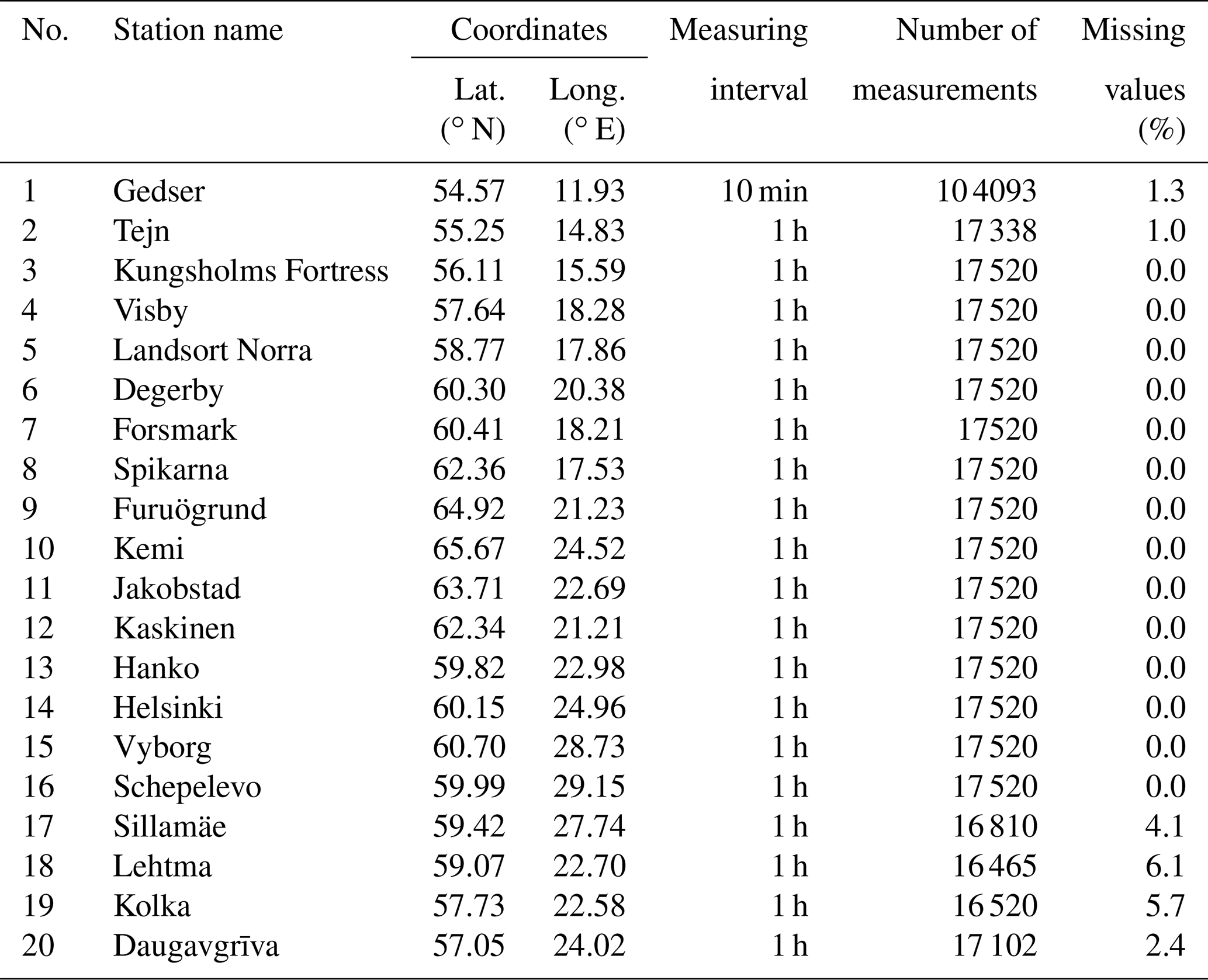
A comparison of the SSH model outputs and the observations from the gauging stations (Fig. 2) demonstrates that the model reproduces the sea level variations in different parts of the Baltic Sea well. The correlation between the simulated and observed time series was higher than 0.79. The absolute bias ranges within 6.7–9.2 cm, which represents 3.7 %–7.4 % of the SSH magnitude at the gauging stations. Most of the model outputs (from 75 % to 90 %) have considerably good accuracy with respect to the P_m parameter (Table 2).

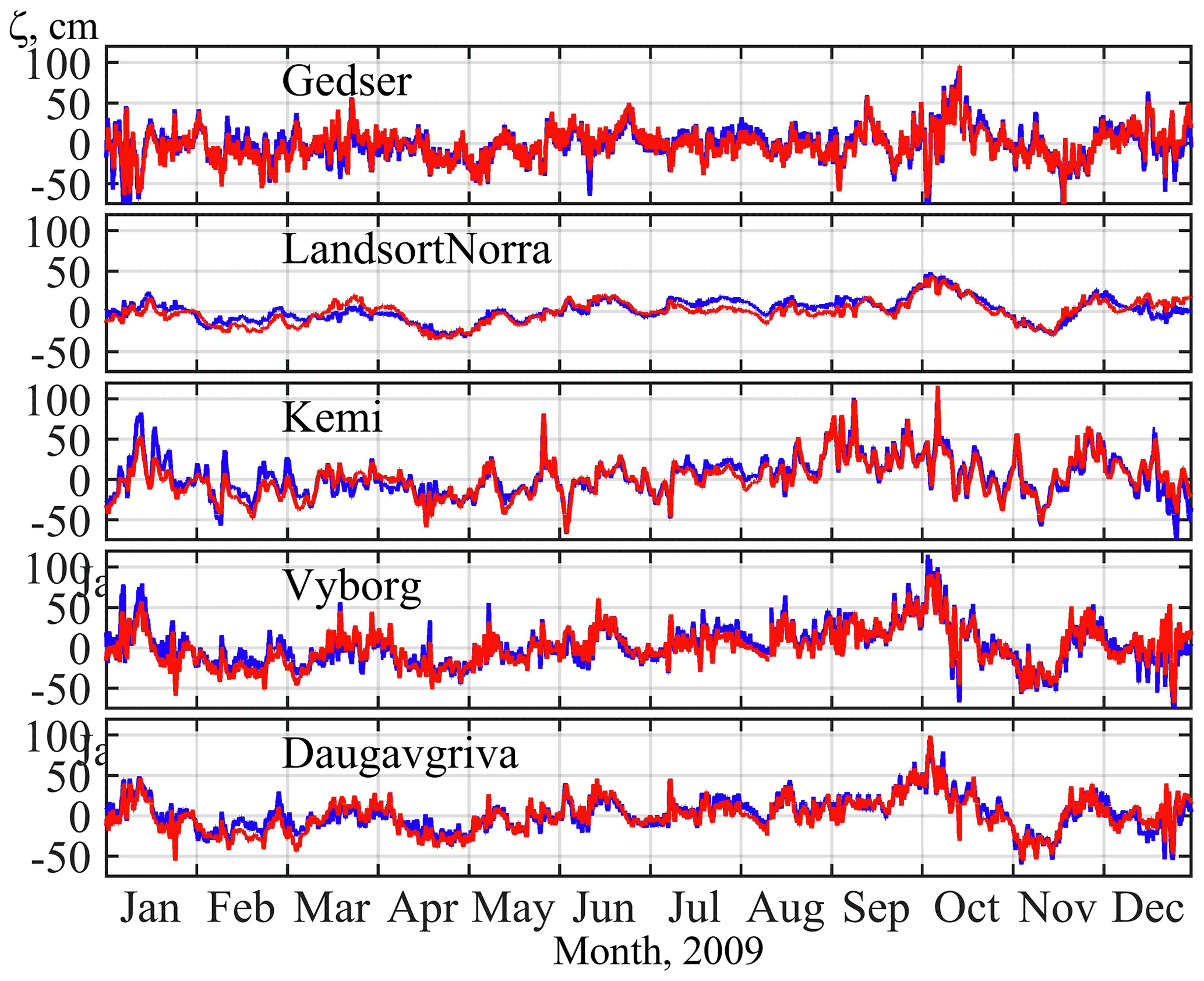
Figure 2 Time series of in situ (blue) and modelled (red) sea level for 2009. The modelled dataset is derived from the basic configuration of INMOM (see Sect. 2.1).

Table 2 Statistical scores evaluating the accuracy of the SSH model simulations.

2.3 Modelling free sea level oscillations in barotropic and baroclinic conditions

To investigate the difference between free sea level oscillations in barotropic and baroclinic conditions, INMOM was run in two different configurations.

In the barotropic configuration, the salt and heat fluxes were set to zero and the water density in the sea state equation depended only on pressure. In the baroclinic configuration, INMOM took into account both salt and heat fluxes, and the water density varied with pressure, temperature, and salinity. In both the barotropic and baroclinic implementations, the Baltic Sea was considered a fully enclosed basin, with no water exchange with the North Sea. The liquid border in the Kattegat Strait was assumed to be solid. This assumption aimed to exclude the effect of external barotropic and baroclinic oscillations coming from the North Sea. River water input and ice conditions were also neglected in both numerical experiments. Under natural conditions, the free sea level oscillations attenuate rapidly due to the dissipative effects of vertical and horizontal viscosity, near-bottom friction, non-linear effects, and Earth's rotation (Proshutinsky, 1993; Zakharchuk et al., 2004). According to theoretical concepts and previous numerical experiments (Leppäranta and Myrberg, 2009; Proudman, 1953; Wübber and Krauss, 1979; Zakharchuk et al., 2004), the relaxation of the Baltic large-scale free sea level oscillations takes several days. In order to be able to characterise the free oscillations with better spectral resolution and in larger spectral range, the sea level dumping factors have to be reduced. In both numerical experiments, the dumping effect was reduced due to (1) setting the coefficients of vertical turbulent viscosity and of bottom friction to zero and (2) setting the coefficient of horizontal turbulent viscosity to the minimum values.

In both the barotropic and baroclinic numerical experiments, the model was perturbed for 10 d (1–10 January 2009) using ERA-Interim reanalysis. The meteorological forcing was then turned off and the simulations were run for 2 years (2009–2010) considering only free dynamic oscillations.

At the end of the atmospheric forcing and the beginning of free sea level simulations, the southern part of the Baltic Sea was under an atmospheric anticyclone centred over central Europe, while the northern part of the sea was affected by a low-pressure system that had developed over the Norwegian Sea. These meteorological conditions resulted in prevailing western winds (Fig. 3a) and finally led to a 50–100 cm sea level increase in the north and east and to 30–50 cm sea level decrease in the south-west (Fig. 3b) parts of the Baltic Sea.

Figure 3 ERA-Interim atmospheric pressure (a) and INMOM SSH (b) for the moment of cessation of atmospheric forcing (10 January 2009, 18:00 LT).

Fourier analyses of the simulated SSH time series were performed using the following decomposition:

$$\begin{array}{}\text{(5)}& f\left(t\right)=Z_{\mathrm{0}}+\sum _{k=\mathrm{0}}^{N/\mathrm{2}}(a_k\cos k\mathit{\omega }t+b_k\sin k\mathit{\omega }t),\end{array}$$

where $\left(\mathit{\omega }=\frac{\mathrm{2}\mathit{\pi }}{T}\right)$, f(t) is the sea level time series, N is the time series length, T is the period, t is the time, a_k is the coefficient at frequency ω, Z₀ is the average of the sea level time series, and k is the coefficient number.

The phase (F_k) and amplitude (A_k) were calculated using Eq. (5) for each model node, and their spatiotemporal distribution was analysed.

$$\begin{array}{}\text{(6)}& A_k=\sqrt{a_k^{\mathrm{2}}+b_k^{\mathrm{2}}},F_k=\arctan \left(b_k/a_k\right)\end{array}$$

The wave phase velocity (C) was estimated using the phase difference between adjacent nodes:

$$\begin{array}{}\text{(7)}& {\displaystyle }{C}_x={\displaystyle \frac{\mathrm{\Delta }x\cdot \mathrm{360}}{T\mathrm{\Delta }{F}_x}},C_y={\displaystyle \frac{\mathrm{\Delta }y\cdot \mathrm{360}}{T\mathrm{\Delta }{F}_y}},\text{(8)}& {\displaystyle }C=\sqrt{C_x^{\mathrm{2}}+C_y^{\mathrm{2}}},\end{array}$$

where C_x and C_y are zonal and meridional components of the wave phase velocity, ΔF_x and ΔF_y are the zonal and meridional phase difference in degrees, respectively, and T is the period.

The estimation of the phase speed was performed only for regions where A_k>0.67σ (Guide, 1994).

$$\begin{array}{}\text{(9)}& \mathit{\sigma }=\sqrt{{\displaystyle \frac{A^{\mathrm{2}}}{\mathrm{2}}}},\end{array}$$

where A is the field average sea level amplitude at each frequency ω.

3 Comparison of simulations of free barotropic and baroclinic sea level oscillations

3.1 Free barotropic oscillations

In general, simulated free barotropic sea level oscillations in the Baltic Sea range within 3–15 cm depending on the region (Fig. 4). The maximum amplitudes are noted in the eastern Gulf of Finland. The minimum values occur in the central part of the Baltic Proper.

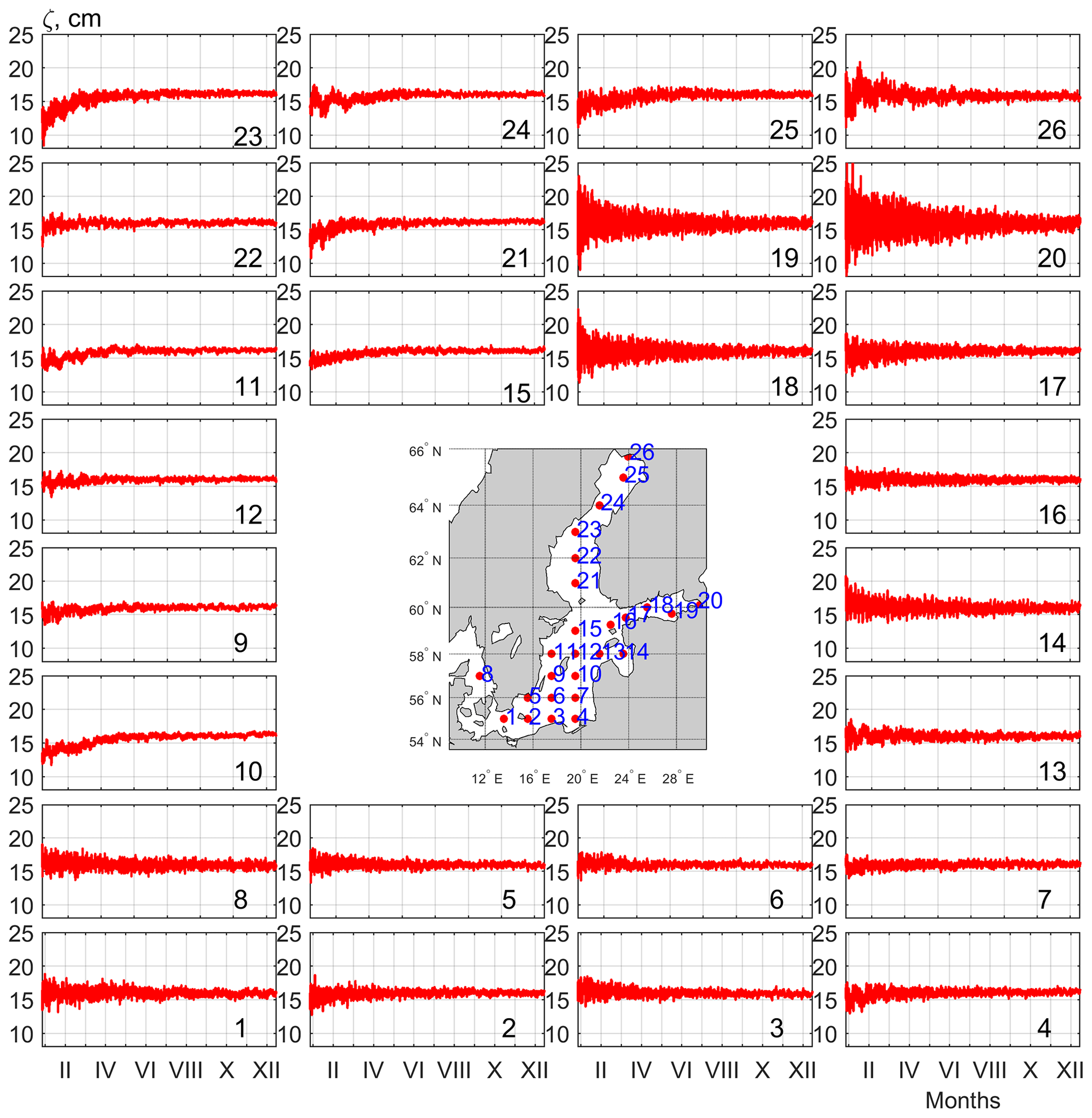
Figure 4 Time series of free barotropic sea level oscillations at selected points simulated by INMOM. Locations of points are shown on the map.

The standard deviation (σ_m) of the sea level estimated for each grid node can be used for the characterisation of the oscillation intensity. The spatial distribution of the σ_m values demonstrates that the highest barotropic oscillations (σ_m of 2.5–5 cm) can be found in the Neva Bay of the Gulf of Finland, in the northern Bay of Bothnia near Hailuoto island, as well as in the Kalmar Strait near the southeast Swedish coast (Fig. 5). Barotropic oscillations of medium intensity (σ_m of 1–2 cm) are observed in the Pärnu Bay of the Gulf of Riga, northeast of the Baltic Proper, near Rügen island, as well as in the Danish straits and Kattegat Strait. Oscillations of medium intensity occur in areas of local uplifts in the Baltic Proper, in the areas of the Ulvö Deep, the Landsort Deep, the Northern Deep, and the Gotland Deep. These local spots have not been observed in previous experiments to be effectuated using a shallow-water model (Jönsson et al., 2008). In the shallow-water equations, the water movement is independent of the vertical coordinate. Sea level fluctuations are generated only due to full flux divergence and surface slope related to geostrophic balance. In regions with sharp bathymetry (uplifts, sills, deeps), the generation of relatively high perturbations of the vertical component of the speed of barotropic flux is probable. These perturbations may not be negligible and, presumably, affect sea level fluctuations.

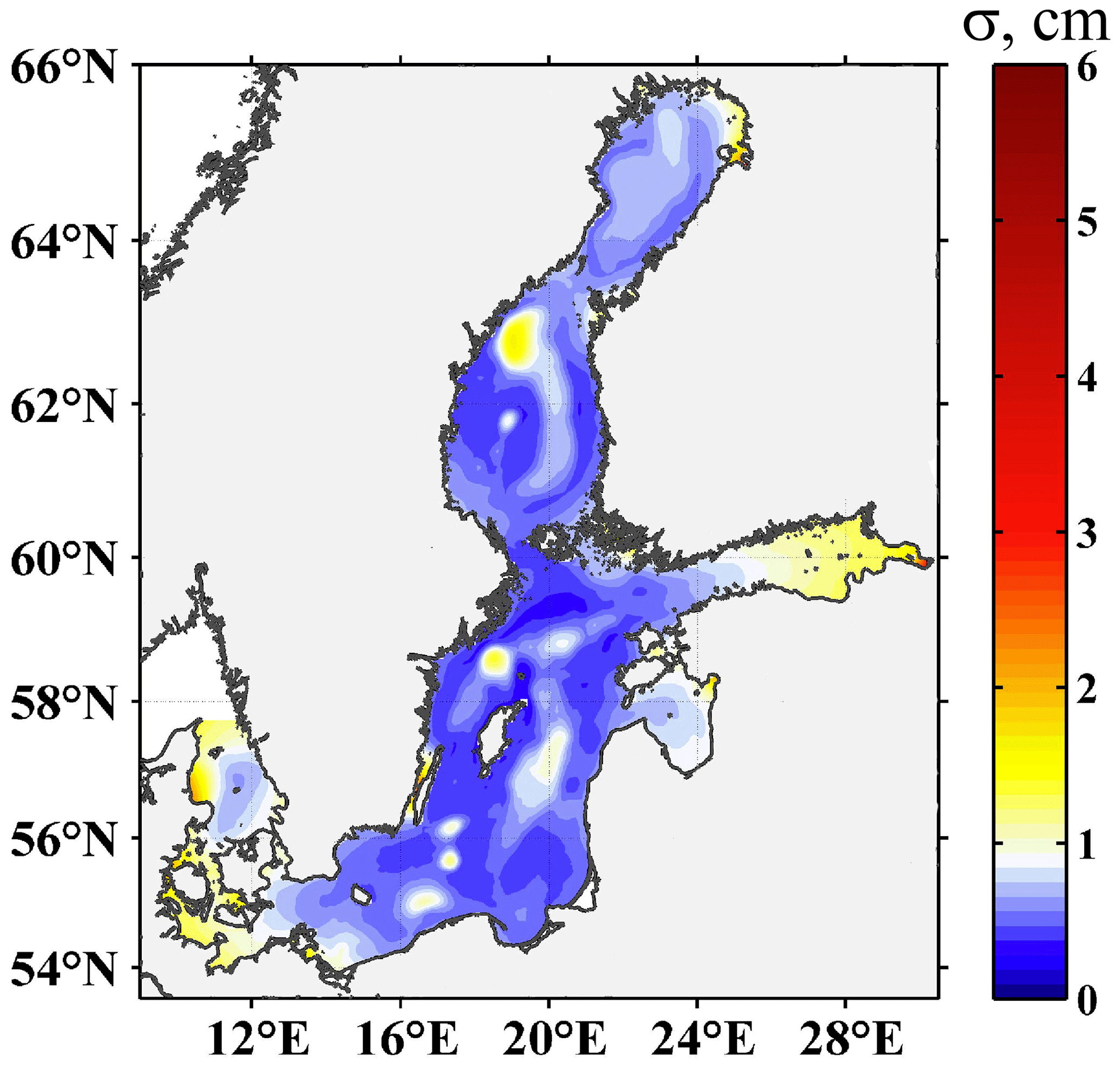
Figure 5 Sea level standard deviation (σ) for free barotropic oscillations simulated by INMOM.

The Fourier analysis of the simulated time series of free barotropic sea level oscillations (Fig. 6) indicates that amplitude peaks frequently occur at periods of 13, 15–16, 19, 23, 27, 29, 41, and 44 h. Near the Gulf of Finland and in the southeast Baltic Proper, the period of the highest amplitude peak is 13 h. In the inner Gulf of Finland, oscillations of 27 h periods became prevalent. The barotropic free oscillations of this period dominate in the northern Gulf of Bothnia and south-western Baltic Proper. Other significant oscillations of 15, 23, 29, and 41 h are also observed in the Gulf of Finland. However, their amplitude is 2–4 times lower than that of 27 h period oscillations.

Figure 6 Amplitude spectra A(ω) of free barotropic oscillations in different parts of the Baltic Sea. Numbers above the peaks show oscillation periods in hours. Locations of points are shown on the map.

In the south-eastern and eastern Baltic Proper, free barotropic oscillations of 13 and 41 h periods have the highest amplitudes. In the centre of the Bothnian Sea, the dominant oscillation has a 19.5 h period. In the Gulf of Riga, the highest amplitude was observed as 23 h barotropic oscillations. This result differs from the 17 h period found in the study by Jönsson et al. (2008) based on the shallow-water model.

Nevertheless, a portion of our results is consistent with those determined by a numerical experiment conducted by Wübber and Krauss (1979), where, similar to our study, the effect of the Earth's rotation was taken into account. These authors identified eigenoscillations with periods of 31.0, 26.4, 22.4, 19.8, 17.1, and 13.0 h. In our experiment, the corresponding periods were 31, 27, 23, 20, 16, and 13 h. Moreover, due to the more sophisticated 3-D model, higher spatial resolution of the grid, and a longer period of simulations (716 d), we were able to improve both the spectral resolution of the simulated time series and their spectral range. We identified additional free barotropic oscillations of periods of 44, 41, 37, 29, 21, 16, and 15 h that have not been noted previously.

An analysis of the spatial distribution of the amplitude and phase of free barotropic oscillations with periods of 13, 27, and 41 h (Fig. 7) demonstrates that due to the Earth's rotation and the enclosed configuration of the sea, these oscillations transform into progressive–standing waves (PSWs). Similar to the amphidromic systems of tidal waves (Nekrasov, 1975; Pugh, 1987; Voynov, 2003), there are no sea level oscillations in the PSW nodes, while in the PSW, the oscillations are maximised. The progressive–standing waves of 13 h periods have 10 nodes (Fig. 7a). Their maximum amplitudes are observed in their antinodes located in the Danish straits and eastern Gulf of Finland.

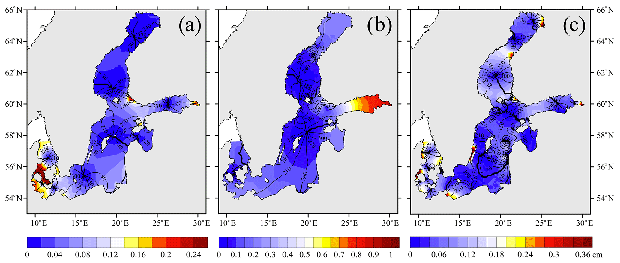
Figure 7 Maps of amplitudes (in cm) and phases in degree (isolines) of free barotropic sea level oscillations with 13 h (a), 27 h (b), and 41 h (c) periods.

The locations of our 13 h amphidromic systems in the gulfs of Bothnia, Finland, and Riga agree well with the results found by Wübber and Krauss (1979) for the 13.04 h eigenoscillations. However, for the Baltic Proper, our systems (near the Fårö and Bornholm deeps) are shifted by 200 km toward the northeast. Another significant difference is the direction of isophase rotation, which in our experiment occurs clockwise, while Wübber and Krauss (1979) suggested an anticlockwise rotation.

Free barotropic oscillations of 27 h periods have two predominant amphidromic systems: one is in the Bothnian Sea and the second is to the northeast of Gotland island (Fig. 7b). Their locations are consistent with the location of the corresponding eigenoscillation of the 26.4 h period of Wübber and Krauss (1979). Our simulations allowed the detection of several more degenerate amphidromic systems of 27 h periods, which have not been reported by previous studies. Degenerate amphidromic systems were found in the northern Bothnian Sea, the Sea of Åland, the central and south-eastern parts of the Gulf of Bothnia, at the exit of the Gulf of Finland, and in the Great Belt and Sound straits. The PSW antinodes with 27 h periods have variable amplitudes, with the highest amplitude located in the eastern Gulf of Finland. Antinodes with lower amplitudes are situated in the northern Gulf of Bothnia, to the southeast of the Åland Islands, in Pärnu Bay of the Gulf of Riga, and in the south-western Baltic Proper. In contrast to the 13 h amphidromic systems, the isophase rotation in the main 27 h systems occurs anticlockwise.

Free barotropic oscillations of 41 h periods are characterised by larger amounts of amphidromic systems (Fig. 7c). Their primary systems are detected in the northern and central Gulf of Bothnia, Bothnian Sea, eastern Gulf of Finland, Kattegat Strait, and Danish straits. Numerous degenerate amphidromic systems can be seen in the north, east, and central parts of the Baltic Proper, along its southern coast, the easternmost part of the Gulf of Finland, and in the Danish straits. The amplitude of the free 41 h oscillations is 2 times lower than that of the 27 h period waves. The most noticeable PSW antinodes are localised within the narrow areas of the coastal zones in the northern and eastern parts of the Gulf of Bothnia, in the Neva Bay of the Gulf of Finland, along the western, eastern, and south-western coasts of the Baltic Proper, as well as in the Danish and Kattegat straits. The isophases of 41 h oscillations rotate in a clockwise direction, similar to the 13 h period waves.

An estimation of the phase speed (C) of the PSW using Eqs. (2) and (3) demonstrates that C reduces with an increase in the wave period (Fig. 8). For the 13 h PSW, the phase speed can reach 40 m s⁻¹, for the 27 h PSW, only 19 m s⁻¹, and for the 41 h PSW, it can reach 13 m s⁻¹. In areas where ΔF_x and ΔF_y are equal to zero (white areas in Fig. 8), the standing wave component prevails.

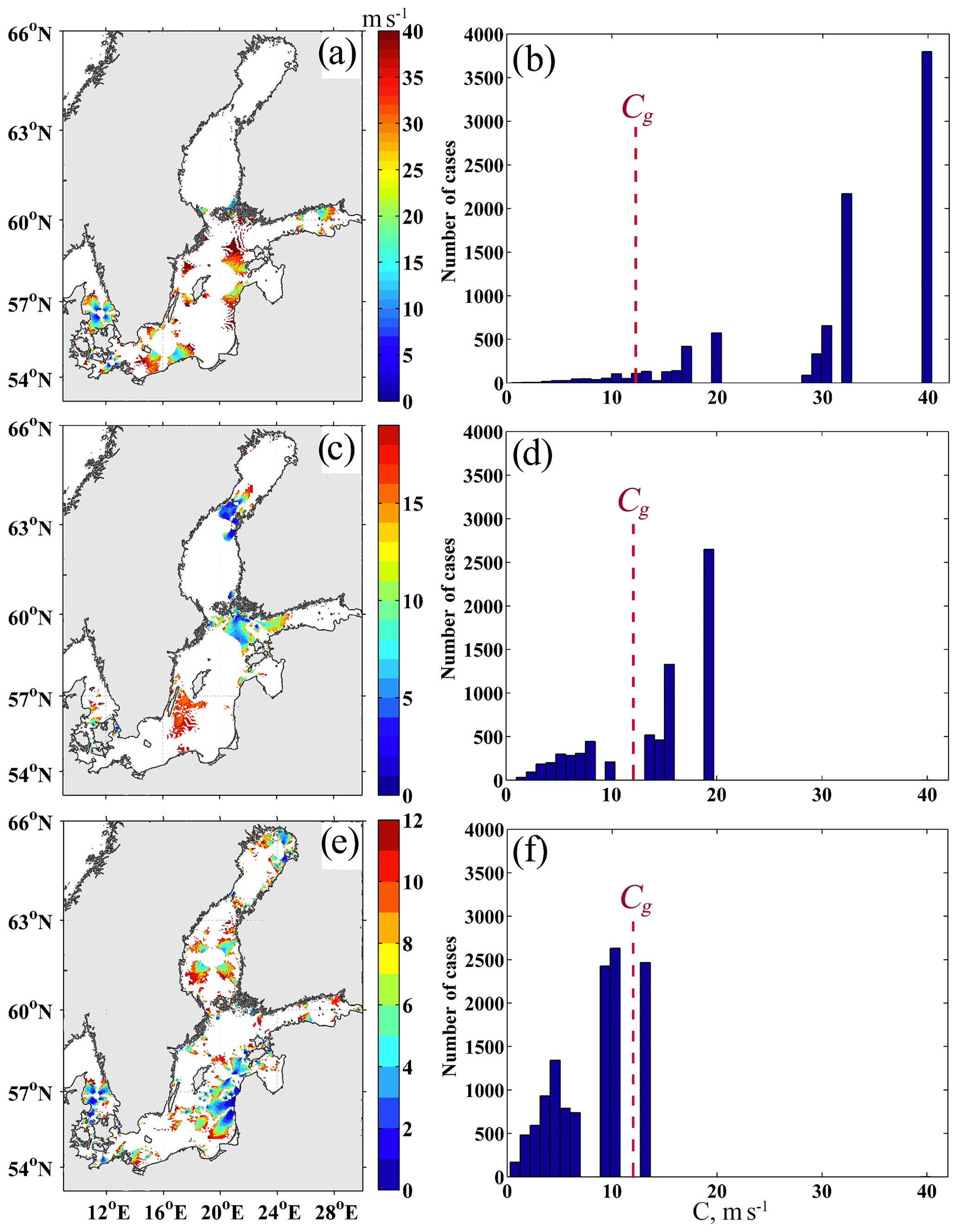
Figure 8 Maps and histograms of phase speed of barotropic progressive–standing waves of 13 h (a, b), 27 h (c, d), and 41 h (e, f) periods. In the regions coloured in white, the estimated phase speed is equal to zero. The dashed line on the histogram plots indicates minimum theoretical value of phase speed of barotropic gravity wave (C_g).

The average depth of the Baltic Sea and its main gulfs varies from 15 to 77 m, while the maximum values reach 14–458 m (Leppäranta and Myrberg, 2009). Under these conditions, the theoretical phase speed of the barotropic gravity wave in the Baltic Sea, calculated using the expression $C_g=\sqrt{gH}$ (where H is the depth and g is the acceleration due to gravity), ranges between 12 and 67 m s⁻¹. Most of our C estimates for the 13 h waves are within this theoretical range (Fig. 8b). For only 70 % of the detected 27 h waves, the phase speed agrees with the theoretical values (Fig. 8d), while among the PSWs of a 41 h period, waves that are lower than the theoretical phase speed dominate (Fig. 8f).

3.2 Free sea level oscillations in baroclinic conditions

In stratified basins along with high-frequency (daily and hourly scales) oscillations, the low-frequency free oscillations of the seasonal scale are also generated after the meteorological forcing ceases. These phenomena have periods from several months to 1 year and reach 30–35 cm in range (Fig. 9).

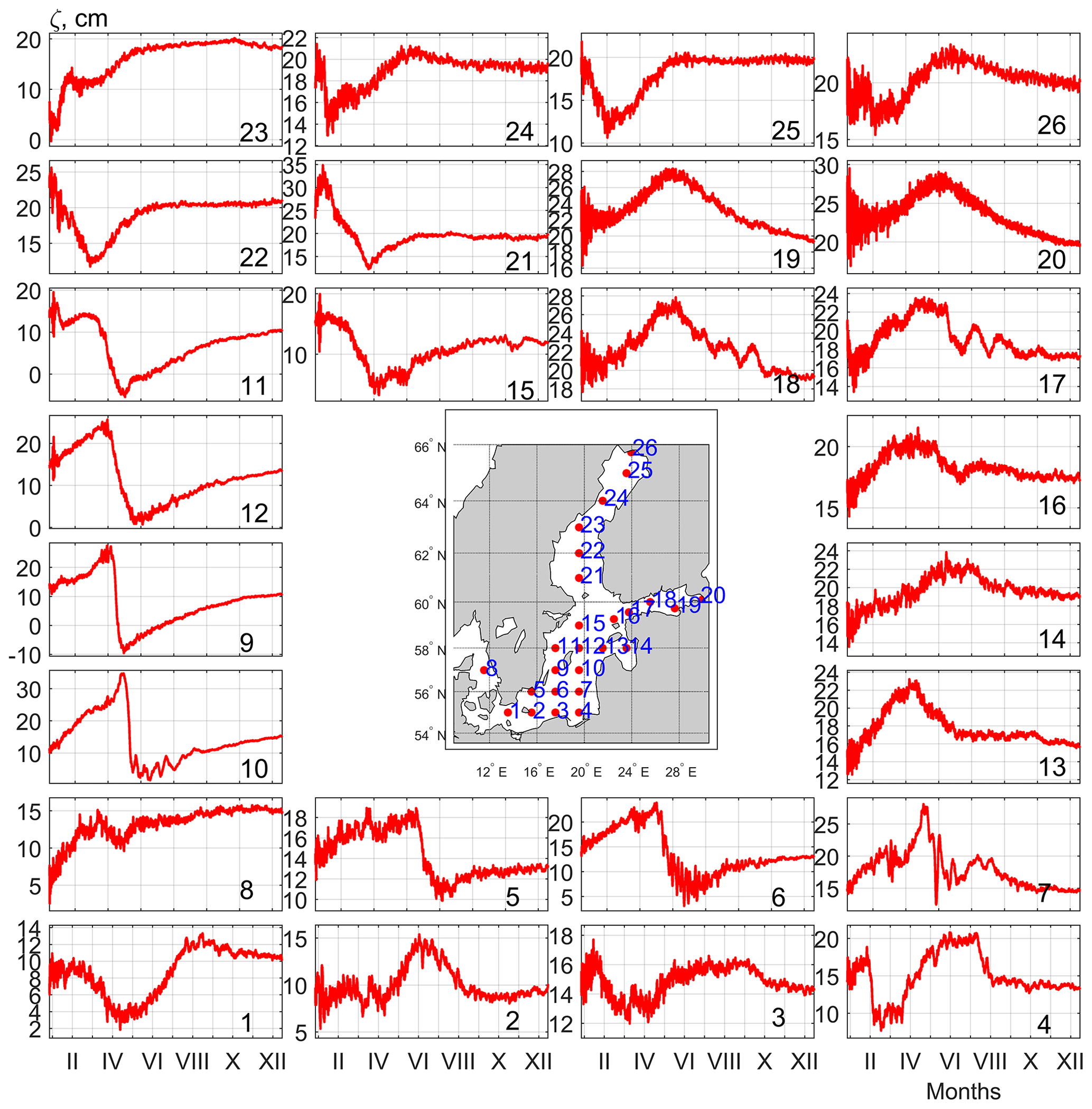
Figure 9 Time series of free sea level oscillations in baroclinic conditions at selected points simulated by INMOM. Locations of points are shown on the map.

The spatial distribution of the standard deviation of the amplitudes of the free oscillations in the baroclinic sea (Fig. 10) demonstrates that the location of the zones with a high SSH variability is similar to that found in the barotropic experiment. These are the deep-water basins of the Baltic Proper: Landsort Deep, Fårö Deep, Northern Deep, and Gotland Deep, as well as the Ulvö Deep in the Bothnian Sea. The σ_m values in the baroclinic experiment were 4–6 times higher than in the barotropic study. We also identified several zones of moderate SSH variability, which were not detected in the barotropic simulations. They are situated in the south-eastern Bothnian Sea, central Gulf of Finland (off the Narva Bay), the straits between the Öland and Gotland islands, and central Arkona Basin.

Figure 10 Sea level standard deviation (σ) for free oscillations in the baroclinic sea, simulated using INMOM.

The Fourier analysis demonstrates that in baroclinic conditions, the maximum energy concentrates mostly at low frequencies. However, the differentiation of distinct peaks in low-frequency bands is problematic (Fig. 11).

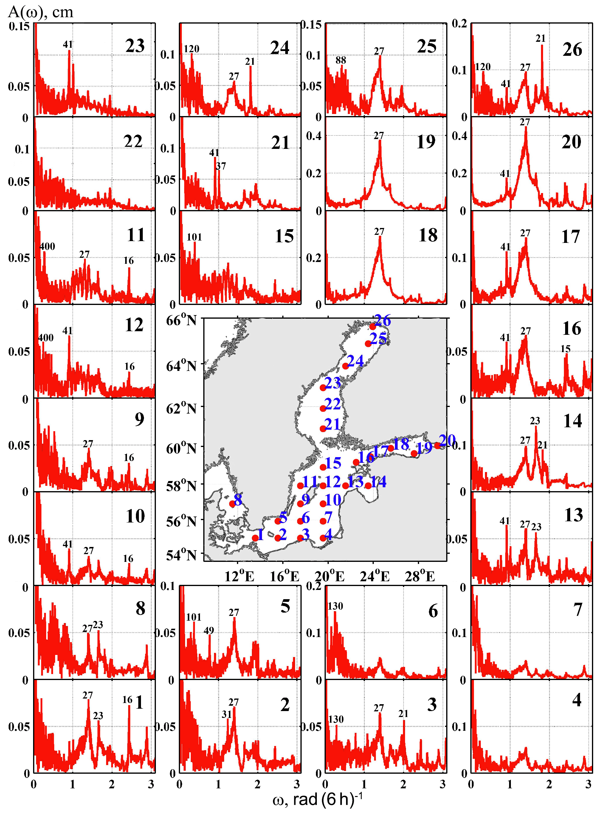
Figure 11 Amplitude spectra A(ω) of free oscillations in baroclinic conditions in different parts of the Baltic Sea. Numbers above the peaks show oscillation periods in hours. Locations of points are shown on the map.

In higher frequencies, the energetic maximums correspond to those found in the barotropic experiments (e.g. to peaks with periods of 13, 19, 23, 27, and 41 h). The difference with the barotropic experiment consists of a decrease in the peak amplitude along with an increase in width. This difference could be explained by the following two factors: (1) the stratification for barotropic free sea level oscillations can work as a dissipative factor; (2) when a barotropic current interacts with sharp bathymetry, the vertical component of the current significantly increases. This component affects the pycnocline and generates baroclinic oscillations with frequencies close to the barotropic oscillations. The resulting oscillations became amplitude modulated and their spectral peaks broaden.

For comparison with the barotropic experiment, the spatial distribution of the amplitudes and phases of the 13, 27, and 41 h oscillations in baroclinic conditions is shown in Fig. 12. In a stratified sea, the amplitude of the 13 and 27 h oscillations is 2 times lower. For lower-frequency waves (41 h), the difference with barotropic conditions is negligible. The highest amplitudes for the 13 h periods are observed in the eastern Gulf of Finland and in Vyborg Bay (Fig. 12a). In the stratified environment, the 13 h amphidromic systems disappear in the Gulf of Bothnia and Gulf of Finland, as well as in the central Baltic Proper. The systems remain detectable only in the southern Baltic Sea and in the Kattegat Strait. Free oscillations of 27 h periods in the baroclinic conditions reached the maximum in the eastern Gulf of Finland (Fig. 12b). The 27 h amphidromic system is observed only in the central part of the Baltic.

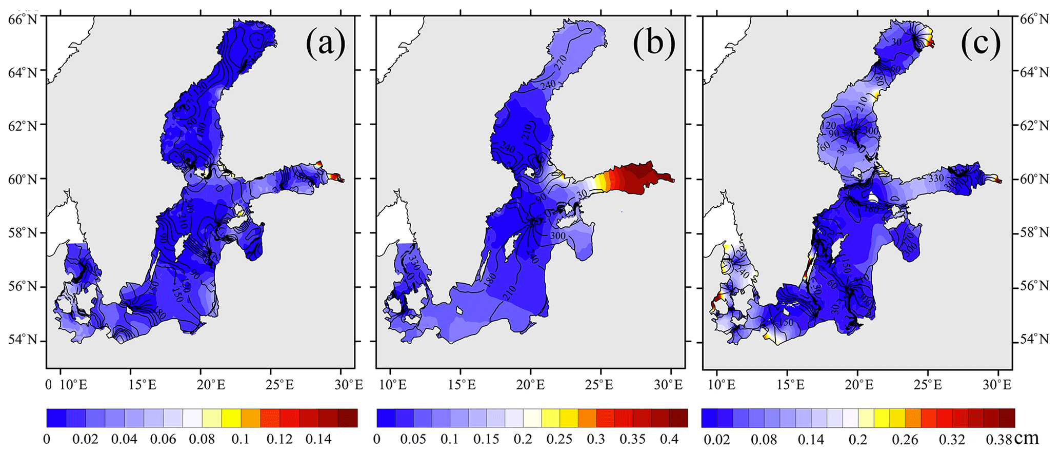
Figure 12 Maps of amplitudes (in cm) and phases in degrees (isolines) of free sea level oscillations with 13 h (a), 27 h (b), and 41 h (c) periods in the baroclinic sea.

The spatial structure of the 41 h free oscillations in the baroclinic conditions was similar to that found in the barotropic experiment. The oscillations of higher intensity are observed within small coastal areas in the north and east of the Gulf of Bothnia, in the Neva Bay of the Gulf of Finland, along the west and south-west coasts of the Baltic Proper, as well as in the Danish and Kattegat straits (Fig. 12c). The location of the 41 h amphidromic systems in the baroclinic conditions in many areas (north of the Gulf of Bothnia, the Bothnian Sea, east of the Gulf of Finland, the Kattegat Strait, and the Danish straits) is similar to that found in the barotropic experiment. However, in stratified conditions, the degenerate amphidromic systems change. One system in the east of the Baltic Proper disappears, while a new appears in the south-eastern section of the sea (Fig. 12c).

The phase speed of the PSW movement in the baroclinic conditions varies within 2–37 m s⁻¹ for the 13 h waves, 1–20 m s⁻¹ for the 27 h waves, and 1–13 m s⁻¹ for the 41 h waves (Fig. 13).

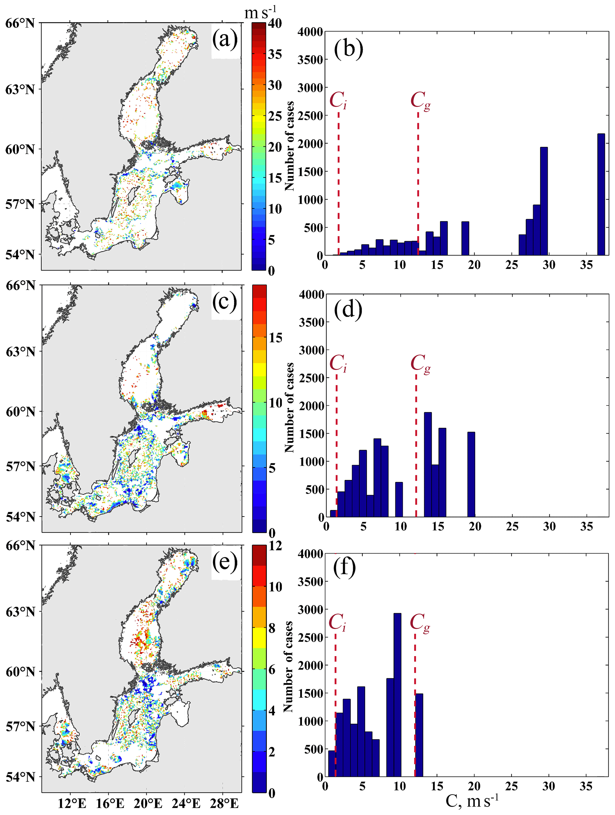
Figure 13 Maps and histograms of phase speed of progressive–standing waves of 13 h (a, b), 27 h (c, d), and 41 h (e, f) periods in the baroclinic sea. In the regions coloured in white, the estimated phase speed is equal to zero. The dashed line on the histogram plots indicates maximal theoretical value of phase speed of baroclinic gravity waves (C_i) and minimal theoretical value of phase speed of barotropic (C_g) gravity waves.

To interpret the detected free sea level oscillations in baroclinic conditions, we compared the estimated phase speed of the modelled oscillations with the theoretical phase speed values of the baroclinic gravity waves. The theoretical dispersion relation of an internal gravity wave (C_i) calculated for the 1.5-layer model (Carmack and Kulikov, 1998) can be estimated using the expression $C_{\mathrm{i}}=\sqrt{g^{\prime }{h}^{\prime }}$, where g is replaced by $g^{\prime }=\frac{\mathrm{\Delta }\mathit{\rho }}{\mathit{\rho }}g$ (ρ is mean seawater density, Δρ is difference in the densities between two layers, and h^′ is upper sea layer depth).

Using the Copernicus data of the vertical distribution of seawater density for 2009–2010, we estimated the phase speed of the internal gravity waves (C_i) for the entire Baltic Sea. For variables ranging from 2 to 60 m (h^′), 3.0–40 × 10⁻⁴ ($\mathrm{\Delta }\mathit{\rho }/\mathit{\rho }$), and 2.9–39 × 10⁻³ m s⁻² (g^′), the phase speed of the internal gravity waves must vary within 0.08–1.53 m s⁻¹.

Our estimations of the phase speed (C) of free oscillations in the baroclinic medium using Eqs. (7) and (8) for waves with 13, 27, and 41 h periods do not coincide with the range of theoretical phase speeds of the internal gravity waves (C_i) in the Baltic Sea. Most of our C estimations for the 13, 27 h, and a significant portion of the 41 h baroclinic oscillations are within the range of theoretical values calculated for the barotropic conditions (see Sect. 3.1).

The spatial structure of free baroclinic oscillations of 89 and 358 d (Fig. 14) agrees well with the spatial distribution of the sea level standard deviation for the free oscillations in the baroclinic sea (Fig. 10). This means that the overall spatial structure of the free oscillations in baroclinic seas is determined mostly by oscillations at seasonal scales. The highest amplitudes of the long-period waves are observed in the deep regions of the Baltic Proper and Bothnian Sea. Moreover, a significant spatial variability in their phases can be noted.

Figure 14 Amplitudes in cm (colour) and phases in degrees (co-tidal lines) of the free sea level oscillations in the baroclinic sea on periods of (a) 358 d and (b) 89 d.

Nodal lines of these waves traverse the sea between the coasts in different parts. In areas of isophase condensation, where the amplitudes of sea level oscillations are near zero, the phase can reverse to the opposite. In other areas, the phase of 358 d oscillations can change gradually. This confirms the likely presence of a low-frequency progressive component of wave movement, which is oriented mostly in the southern direction (Fig. 14a).

Free baroclinic oscillations of 89 d have degenerate amphidromic systems in the south-west, south, and north-west Baltic Proper. These systems rotate in a anticlockwise direction (Fig. 14b). The phase velocity of the seasonal PSWs varies within 0.01–0.07 m s⁻¹ and 0.01–0.24 m s⁻¹, respectively, for 358 and 89 d oscillations. For 358 d waves, our estimations of the phase speed are significantly lower than those of the theoretical internal gravity waves (C_i). For 89 d waves, the part of our estimations belongs to the range of phase speed of internal gravity waves.

Regarding the theoretical phase speed of the internal gravity waves (C_i), these values are significantly lower for longer waves and belong to the theoretical range for waves of the shorter period (Fig. 15).

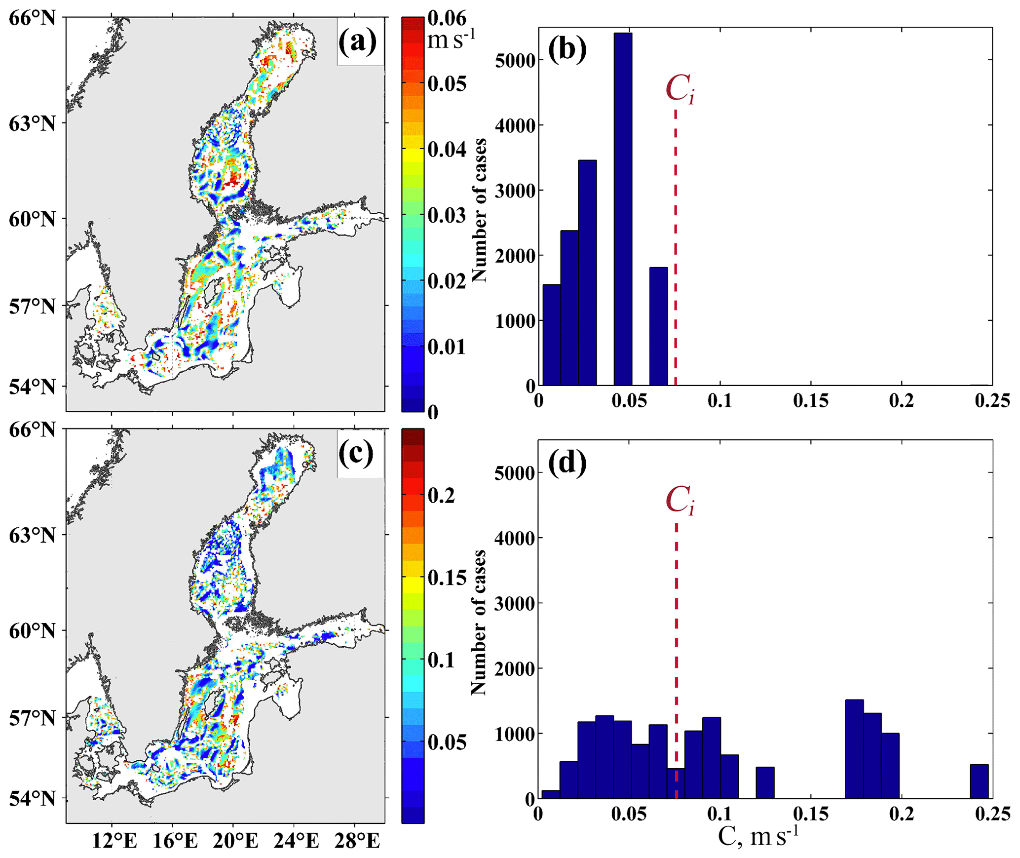
Figure 15 Maps and histograms of phase speed (m s⁻¹) of progressive–standing waves of 385 d (a, b) and 89 d (c, d) periods. In the regions coloured in white, the estimated phase speed is equal to zero. The dashed line on the histogram plots indicates minimum value of theoretical phase speed of baroclinic gravity waves.

4 Discussion

Our numerical experiments based on a three-dimensional hydrodynamic model demonstrated that after the cessation of meteorological forces, the return of the Baltic Sea water mass to equilibrium in barotropic and baroclinic conditions is different.

In barotropic conditions, the most intense free oscillations occur on a timescale of 13, 15–16, 19, 23, 27, 29, 41, and 44 h. The highest oscillations with amplitudes of 7.5 cm occur in the head of the Gulf of Finland, Gulf of Bothnia, and in the Kalmar Strait.

In baroclinic conditions, high-frequency free oscillations (periods of 13, 19, 23, 27, and 41 h) are also observed. However, their role is minor, with amplitudes that are significantly lower than the amplitude of lower-frequency oscillations. In baroclinic conditions, oscillations of periods from several months to 1 year, with total amplitudes reaching 15–17 cm, appear (Fig. 9). The area with the highest amplitudes of free baroclinic oscillations is located in the deep part of the Baltic Proper, where the highest gradients of water density are observed (Terziev et al., 1992).

Barotropic and baroclinic free sea level oscillations with periods of 13–41 h represent multi-node progressive–standing waves with amphidromic systems rotating in different directions. The speed of the isophase rotation in barotropic amphidromic systems of 13 and 27 h periods is close to the theoretical phase speed of barotropic gravity waves, while the phase speed of the amphidromic systems with a 41 h period is lower than that of gravity waves. In baroclinic conditions, the values of progressive–standing wave phase speeds usually disagree with the theoretical values of gravity wave phase speed estimated for stratified sea.

Correct identification of the described free barotropic and baroclinic oscillations in the Baltic Sea can help to explain many large-scale variabilities of different physical characteristics (for example, large-scale sea level changes).

According to theoretical investigations by LeBlond and Mysak (1978), a sea basin is characterised by its own set of frequencies of barotropic and baroclinic oscillations. These oscillations refer to two classes. The eigenoscillations of the first class are long gravity waves representing longitudinal waves. In no-boundary ocean conditions and under the effect of the Earth's rotation, this type of wave is generated with frequencies that are above the local inertial frequency. An introduction of a boundary results in trapping the wave energy and generating trapped gravity Kelvin waves (Pedlosky, 1979). The Kelvin wave is the only wave type existing in both band frequencies, above and below the inertial frequency (Pedlosky, 1979). Kelvin waves always propagate anticlockwise in the Northern Hemisphere and clockwise in the Southern Hemisphere.

Eigenoscillations of the second class are planetary waves. Among them, Rossby and topographic waves have been extensively investigated (LeBlond and Mysak, 1978). Rossby waves are horizontal transverse waves that are generated in the frequency band, which are below inertia frequencies (Pedlosky, 1979). Rossby waves always propagate westward, while topographic waves move along isobath lines and leave sharp bathymetry from their right in the Northern Hemisphere and from their left in the Southern Hemisphere.

In semi-enclosed sea basins, the mechanism of wave reflection may have an significant effect on the propagation of long waves and can lead to the generation of progressive–standing modes of gravity and planetary waves (LeBlond and Mysak, 1978; Nekrasov, 1975; Pedlosky, 1979).

An earlier theoretical investigation of the dynamics of topographic Rossby waves in enclosed basins (Buchwald, 1973; LeBlond and Mysak, 1978; Pedlosky, 1979) demonstrated that they may have characteristics of both standing and progressive waves. Two types of node lines were observed in the Longuet-Higgins (1965) study during the experiment in a rectangular basin: lines approximated by an envelope function with nodes stable in spatiotemporal domain, as well as lines of progressive waves moving westward with a Rossby wave phase speed.

Theoretical studies of long gravity waves in enclosed or semi-enclosed basins that account for the Earth's rotation have shown that these waves transform into multi-node progressive–standing Kelvin waves (Nekrasov, 1975; Pugh, 1987; Taylor, 1922). The overall effect of the Earth's rotation on free oscillations is to vitiate the development of fixed nodal lines and to atrophy them into nodal points or amphidromic centres (Wilson, 1972). Then, an oscillation rotates around the amphidromic centre in the form of a Kelvin wave such that the amplitude increases from zero in its centre to the maximum on basin boundaries. In the Northern Hemisphere, this rotation is anticlockwise and changes to clockwise in the Southern Hemisphere.

Besides the Coriolis force, the opposite rotation of isophases in amphidromic systems may result from the interference of standing waves (Harris, 1904; Nekrasov, 1975; Proudman, 1953; Schwiderski, 1979). Multiple combinations of amplitude, angle, and phase differences of interfering waves are possible and may lead anticlockwise to clockwise rotation.

The analysis of our numerical simulations coincides with the results of these theoretical experiments. The opposite phase rotation is found for progressive–standing waves with a 27 h period (anticlockwise, similar to the Kelvin wave) and for progressive–standing waves with 13 and 41 h periods (clockwise). The comparison of the phase speed of simulated free barotropic oscillations with theoretical values suggests that most of the oscillations with periods of 13 and 27 h are barotropic gravity waves. Other waves with 27 h periods and almost all waves with 41 h periods are likely to be related to barotropic modes of topographic Rossby waves as their phase speed is lower than that of the theoretical barotropic gravity waves, and their period is longer than that of inertial oscillations (about 14 h).

Compared with barotropic conditions, the number and locations of amphidromic systems in a stratified sea change remarkably (Figs. 7a and 12a). By their phase speed, most of the free oscillations in the baroclinic conditions of high (13 h) and medium (27 h) frequencies, as well as a substantial portion of oscillations at a lower frequency (41 h), can be identified as barotropic gravity waves.

Our experiments demonstrate that in a stratified sea, the percentage of relatively slow-moving free waves significantly increases when compared with an unstratified sea. These changes can be associated with the generation of the baroclinic mode of the topographic Rossby waves in a stratified medium. The significant difference in the phase pattern in baroclinic and barotropic conditions (see Sect. 3.2) can be explained by the superposition of the phases of (1) barotropic gravity waves and (2) barotropic/baroclinic modes of the topographic Rossby waves. We also noted that there is no evidence of the existence of the baroclinic mode of long gravity waves in the Baltic Sea because most of our phase speed estimates for the 13 and 27 h oscillations do not agree with the range of theoretical phase speeds of the internal gravity waves estimated for local baroclinic conditions.

Free sea level oscillations at seasonal scales (periods of 3 months to 1 year) have a baroclinic origin, as they appear only in baroclinic simulations. Maximal amplitudes of free oscillations of the 358 and 89 d periods do not exceed 2.5–5.5 cm (Fig. 14). These amplitudes are of the same order as the amplitudes of annual Baltic Sea level variability (4–13 cm) estimated using stationary approximation from the tide gauges (Ekman, 1996; Medvedev, 2014). The phase speed of the oscillations in the 358 d period is lower than the theoretical values for the internal gravity waves and significantly varies from the range of values typical for barotropic gravity waves. We relate these oscillations to the baroclinic mode of topographic Rossby waves. A fraction of waves of the 89 d period are also the topographic Rossby waves. However, the other part of these oscillations has phase speeds (0.01–0.24 m s⁻¹) overlapping with the range of theoretical values of the internal gravity waves (0.08–1.53 m s⁻¹). This part can be identified as a baroclinic gravity wave.

Several studies have demonstrated that amplitudes of seasonal fluctuations in the Baltic sea level have important interannual variability (Barbosa and Donner, 2016; Cheng et al., 2018; Ekman, 1998; Samuelsson and Stigebrandt, 1996; Stramska et al., 2013). Considering that the free oscillations of seasonal-scale frequencies have a baroclinic origin, we hypothesise that they could contribute to the non-stationary nature of these seasonal fluctuations. Major Baltic inflows (MBIs) are well-known sporadic events that import saline waters into the Baltic. In recent decades, their occurrence has changed significantly (Fischer and Matthäus, 1996; Matthäus, 2006). The MBI events, along with the interannual variability of the freshwater input via atmospheric precipitation and river flow, affect the Baltic Sea water mass stratification (Assessment of Climate, 2008). The interannual variability in the stratification, in turn, may affect the frequencies of the baroclinic modes of the Baltic Sea eigenoscillations. As a result, from year to year, the resonance of atmospheric forces with the baroclinic modes of free sea level oscillations can occur at different seasonal-scale frequencies or may not occur at all. This mechanism may be one of the reasons responsible for the unsteady character of the Baltic sea level seasonal variability, and its role will be studied in the future.

5 Conclusion

The results of our numerical simulations of the free sea level oscillations of the Baltic Sea revealed a general similarity, with a distinct difference in the processes of relaxation of sea level oscillation in barotropic and baroclinic conditions.

The predominant common feature is the generation of oscillations in the same mesoscale frequency range (13–41 h) in both the unstratified and stratified sea experiments. These oscillations have the form of single- or multi-node progressive–standing waves with amphidromic systems rotating in opposite directions depending on the oscillation period.

The primary difference between the results of the experiments consists in the generation of sea level baroclinic oscillations of seasonal scales with periods of 89 and 358 d in a stratified sea.

The highest amplitudes of free barotropic oscillations occur in the eastern part of the Gulf of Finland, in the Gulf of Bothnia, in the south-western Baltic Proper, and in the Kalmar Strait. The highest amplitudes of baroclinic oscillations are found in the deep areas with the highest stratification of water masses in the Baltic Proper.

Free barotropic oscillations of periods of 13 and 27 h represent long gravity waves. Most of the 41 h period barotropic oscillations are likely to be the barotropic mode of the topographic Rossby wave.

The essential part of free oscillations of 13–41 h periods in the baroclinic conditions may be regarded as topographic Rossby waves generated in semi-enclosed basins. However, there is a minor part of these oscillations that may represent barotropic gravity waves. We did not find evidence of the existence of the baroclinic mode of long gravity waves at these frequencies.

Regarding free oscillations at a seasonal scale, we suggest that all oscillations of 358 d and half of the oscillations of 89 d are related to the baroclinic mode of the topographic Rossby waves, as their phase speeds do not overlap with the theoretical values estimated for internal gravity waves. However, the other part of 89 d baroclinic oscillations, with their phase speed, is likely to be the baroclinic gravity waves.

Based on the results of our numerical experiments, we can conclude that after the cessation of the atmospheric forcing, the relaxation of the Baltic free sea level oscillations occurs in the form of barotropic and baroclinic modes of progressive–standing gravity waves as well as in the form of topographic Rossby waves. The free baroclinic oscillations contribute significantly to the spectre of the Baltic Sea eigenoscillations. Their role is the most important in seasonal-scale sea level fluctuations.