Effects of marine traffic on sediment erosion and accumulation in ports: a new model-based methodology

The action of propeller-induced jets on the seabed of ports can cause erosion and the deposition of sediment around the port basin, potentially significantly impacting the bottom topography over the medium and long term. If such dynamics are constantly repeated for long periods, a drastic reduction in ships' clearance can result through accretion, or the stability and duration of structures can be threatened through erosion. These sediment-related processes present port management authorities with problems, both in terms of navigational safety and the optimization of management and maintenance activities of the port's bottom and infrastructure.

In this study, which is based on integrated numerical modeling, we examine the hydrodynamics and the related bottom sediment erosion and accumulation patterns induced by the action of vessel propellers in the passenger port of Genoa, Italy. The proposed new methodology offers a state-of-the-art science-based tool that can be used to optimize and efficiently plan port management and seabed maintenance.

1 Introduction

The operational activities of harbors and ports are closely related to the local bathymetry, which must be sufficiently deep to guarantee the regular passage, maneuvering, and berthing of ships. However, ship clearance is often so limited that it threatens the safety of in-port navigation, and ships may even hit the seabed in extreme cases. Therefore, this is a critically important issue that often results in management and maintenance efficiency problems in terms of the bottom and a port's infrastructure in general (Mujal-Colilles et al., 2016; Castells-Sanabra et al., 2020).

The action of a ship's main propellers means that traffic in ports is responsible for generating intense current jets, as noted in Fig. 1. The high velocities induce shear stresses on the sea bottom, which can possibly result in sediment resuspension when they exceed the critical stress point for erosion (Van Rijn, 2007; Soulsby et al., 1993; Grant and Madsen, 1979). Before depositing back onto the seafloor the resuspended sediment may be transported widely around the basin by the combined effects of natural currents, such as those induced by tides, winds, or density gradients, and by vessel-related currents, such as those induced by the propellers or the movement and displacement of ships. Thus, the continuous traffic in and out of ports can result in the displacement of a huge volume of seabed material, which can then induce significant variations in the bathymetry over medium to long timescales. The formation of erosional or depositional trends in specific areas of port basins can potentially result from these variations.

Figure 1 Example of a propeller-induced jet of a moving ship (main propulsion without rudder).

If such dynamics are particularly pronounced and rapid (bottom accretion of the order of tens of centimeters per year or even higher), the port authorities must carry out dredging operations for the maintenance of the seabed, in order to fully recover the clearance and ensure the conditions necessary for undisturbed ship motion, maneuvering, and docking or undocking operations.

Most of the published literature about the effects of ships' propellers on port sediments and structures is experimental, and it has mainly been conducted in laboratories using physical models (Mujal-Colilles et al., 2018; Yuksel et al., 2019). Few practical instruments are available for port authorities that can provide robust and scientifically based analyses and predictions of the relevant processes. Such tools can enable managers to plan specific actions aimed at maintaining the seabed, thereby helping to guarantee the continuity of operational activities of ports and to optimize the use of economic resources. Unplanned maintenance activities usually involve additional costs due to the need to operate under emergency conditions and, in some cases, partially interrupt the service.

The integrated numerical modeling of hydrodynamics and sediment transport represents an important aid to port authorities and, more broadly, to port managers and operators, as suggested by Mujal-Colilles et al. (2018). This can reproduce and thus provide a better understanding of the seabed sediment dynamics induced by ships' propellers over short, medium, and long timescales, thereby establishing what tools are required to ensure the efficient operational maintenance of the seabed.

Propeller-induced jets have mainly been studied using empirical formulas based on specific characteristics of the ships and ports of interest, such as the bathymetry; propeller typology, diameter, and rotation rate; and the ship's draft. The most common approaches are the German method (MarCorm WG, 2015; Grabe, et al., 2015; Abromeit et al., 2010) and the Dutch method (CIRIA, 2007). The resulting induced velocities are usually only considered locally to inform the technical design of mooring structures and the protection of a port's infrastructure. Although various assumptions are introduced through empirical formulas, these approaches are limited and do not fully consider the three-dimensional evolution of the induced jet throughout the water column at any distance from the propeller or at any location of the port. Therefore, these tools are not suitable for the comprehensive management of ports.

We conduct a pilot study of the hydrodynamics and seabed evolution induced by ships' propellers in the passenger area of the port of Genoa (Fig. 2), where the marine traffic involves mainly passenger vessels (ferries and cruise ships, generally self-propelled) and in which the resulting sediment dynamics in terms of erosion and deposition rates are particularly significant: estimated to be of the order of several tens of centimeters per year (as directly estimated and communicated by the port operators and via an analysis of bathymetric surveys). In this study, we propose that the integrated high-resolution numerical modeling of three-dimensional hydrodynamics and sediment transport can be a robust and science-based tool for the optimization and efficient planning of port management and maintenance activities. We propose a new methodology that can be used in a delayed mode and can, thus, reproduce the historical major sediment processes over time, as in this study, or in a prediction mode through the potential implementation of real-time operational services.

The remainder of this paper is organized as follows: in Sect. 2, we introduce our methodology; the data available for the study are presented in Sect. 3; Sect. 4 describes the numerical models used; the results of the numerical simulations are presented and discussed in Sect. 5; and the summary and conclusions of the work are given in Sect. 6.

2 Methods

The study is based on the latest versions of the hydrodynamic and mud transport models MIKE 3 FM (DHI, 2017), which are described in detail in Sect. 3 and in Appendices A and B. A very high resolution was used in the numerical model to realistically reproduce the propeller-induced jet, both in the vertical and in the horizontal, at approximately 1–2 and 5 m, respectively. Together with a non-hydrostatic version of the hydrodynamic model, this enables the processes and dominant patterns of the current field generated by the ships propellers during the navigation and maneuvering inside the port to be reproduced very accurately.

As shown in Fig. 2, 12 docks have been included in the study (marked with orange or red lines indicating ferry or cruise vessels, respectively). The port authority mainly focused on passenger vessels, as they considered their effect on the seabed to be greater than other types of vessels that have much less frequent passage. Moreover, passenger ships generally self-propelled, whereas other vessel types are often driven by tugboats. Therefore, we only simulated passenger ships.

The turning basins in which arriving vessels undergo maneuvers for berthing are represented by the white dashed circles marked “a” and “b” in Fig. 2. Circle a refers to vessels berthing at docks T5 to T11, whereas circle b refers to vessels berthing at docks T1 to T3. Finally, the turning area for vessels arriving at docks D.L., 1012, and 1003 is at the entrance of the port and is not simulated in this study, as it is outside of our area of interest.

The general methodology can be separated into the following four phases:

1. Assessment of the marine traffic during a typical year. This phase is fundamental, as it identifies the typical dynamics of the marine traffic in the different sectors of the port and the characteristics of the ships that have the greatest effect on the hydrodynamics and sediment resuspension on the bottom. These include the size of the ships, the related draft, the dimension of the propellers, and their typical rotation rates. The results of the analysis, which are discussed in detail in Sect. 4.1, also enabled representative synthetic vessels for each berth of the port to be defined.

2. Implementation of a high-resolution three-dimensional hydrodynamic model of the port of Genoa. This numerical hydrodynamic model considered ship routes, both entering and exiting the port, as established through the previous vessel traffic analysis phase. As detailed in Sect. 4.1, 24 simulations of the hydrodynamic model have been implemented, one for each dock and route considered (docking and undocking). The resulting 24 scenarios were then simulated separately. This enabled us to analyze the effect of each vessel's passage on the induced hydrodynamics of the basin. Each hydrodynamic contribution was then used to drive the sediment transport model. This approach does not consider potential simultaneous interactions amongst hydrodynamic patterns generated by different propellers, as we assume that vessels are unlikely to pass in close proximity to one another.

3. Implementation of a coupled sediment transport model. Based on the available data, a numerical model of sediment resuspension and transport for fine-grained and cohesive material was then implemented. The model was combined with the hydrodynamics resulting from the 24 different vessel scenarios. The simulations of the sediment model were conducted separately for the hydrodynamic component.

4. Collating the results and the overall analysis. The effects of the passage of the single vessels on the bottom sediment were then combined in terms of the erosion and deposition resulting from the overall number of passages over the analyzed 1-year period of time. This enabled us to provide aggregated information on the annual sediment dynamics.

We then conducted a semiquantitative calibration and validation of the modeling results through a comparison of the seabed evolution reproduced using the integrated modeling system and the various bathymetric maps derived from surveys of the port topography at approximately 1-year intervals.

The proposed approach assumes that each hydrodynamic and sediment transport simulation uses the same bathymetry as the initial bottom condition. Although this assumption may have implications, as we explain in the results section, it does not compromise the main conclusions of the study.

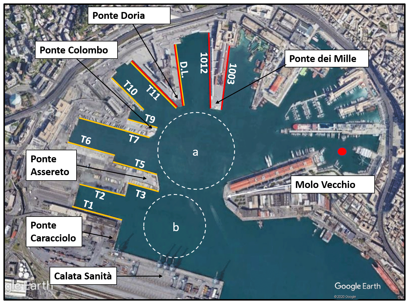
Figure 2 Passenger port of Genoa. The colored lines along the docks refer to the typology of the operating ships: red lines indicate cruise vessels, and orange lines indicate ferries. The names of the docks (in white) are given next to the colored lines. The red dot represents the location of the station where sediment samples with physical information on the grains are available (see Sect. 4.2). The white dashed circles “a” and “b” represent the turning areas for vessels berthing at docks T5–T11 and at T1–T3, respectively. Land background from © Google Earth.

3 Available data and information

Most of the data necessary for this project were provided by the Port Authority of Genoa and Stazioni Marittime SpA, the main port operator in the area.

3.1 Bathymetry

Several bathymetry surveys of the sectors of the port were available at various resolutions. The dataset used for the simulations was obtained by merging the latest available surveys (March–June 2018) of the inner sectors of the port, delivered on a regular grid of 5 m resolution. Figure 3 shows the merged bathymetry for the entire port (left panel) as well as detailed information on Ponte Colombo and the surrounding basin (right panel). The main area of interest for the study (from the line between Calatà Sanità and Molo Vecchio to the end of the port, see Fig. 2) measures approximately 0.60 km² and has an average depth of approximately 13 m. The bathymetry is generally heterogeneous. The wet basins are approximately 10–11 m deep, whereas areas shallower than 10 m are present only in the eastern part of the basin where yachts and noncommercial vessels operate. A deep natural pit is clearly visible a few tens of meters off the right edge of Ponte Colombo and Ponte Assereto, extending approximately 22 m below the water surface. The port authority has designated this area as a preferred site for dumping the sediment resulting from regular maintenance dredging operations of the seabed in sectors where depositional trends are large enough to reduce vessels clearance and to affect the safety of navigation inside the port. This depressed area is also used as a turning area by passenger ferries heading to docks T5, T6, T7, and T9, which cover approximately 50 % of the marine traffic in the basin (see Sect. 4.1). During their maneuveres over this pit, the turning ferries produce intense turbulence, which may reach the newly dumped material resulting from the dredging operations. This material is still loose and can consequently be easily resuspended and transported around the port basin, thereby making the dredging operations ineffective.

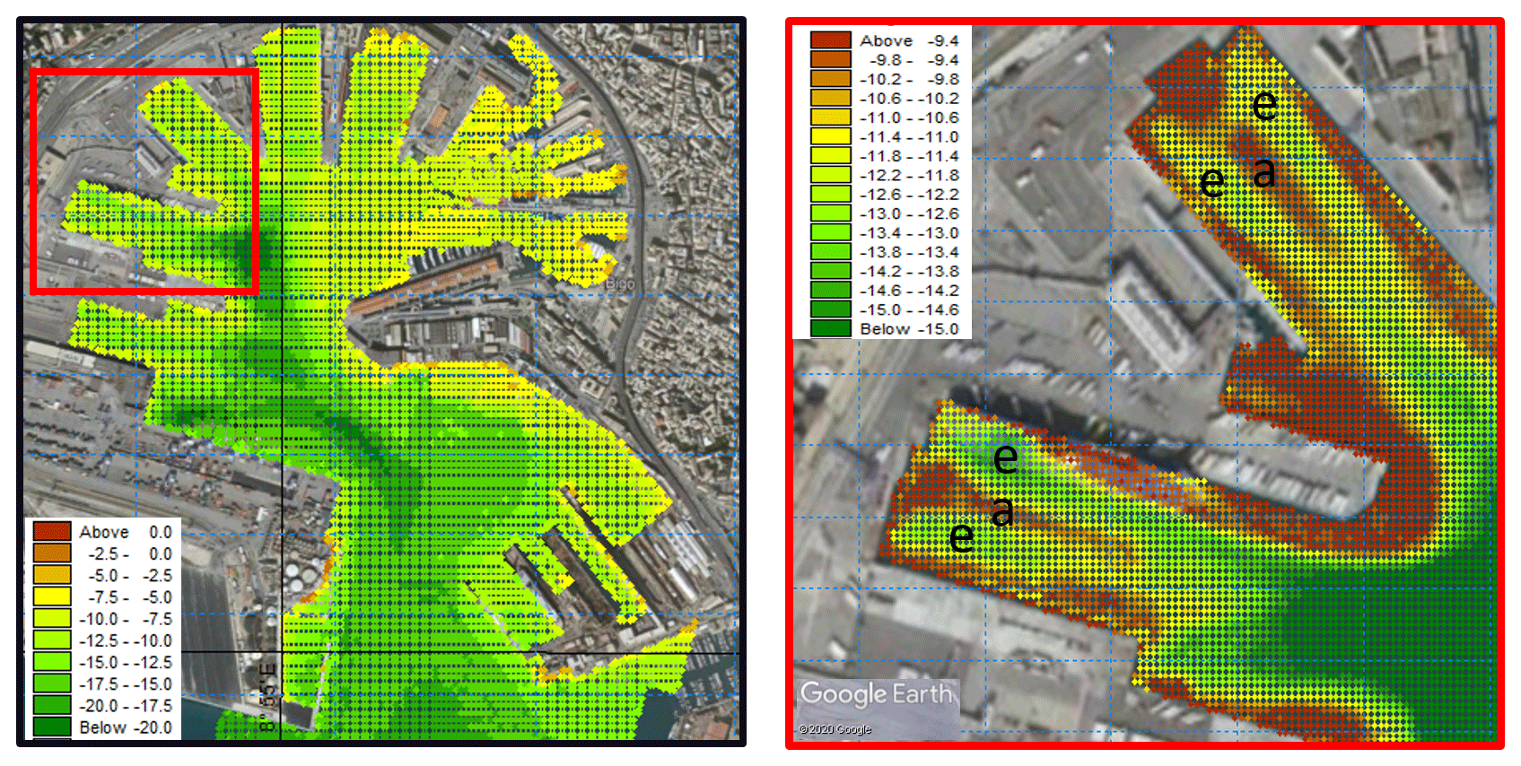
Figure 3 Bathymetry of the port of Genoa. Entire passenger port (left panel) and a zoom in of Ponte Colombo and the surrounding basins (T5–T11, right panel). Land background from © Google Earth.

The bathymetry presented in the right panel of Fig. 3 follows the pattern of erosion and accumulation common to wet basins confined among docks. The propeller activity when vessels leave or approach the berth induces areas of erosion, identified by channels of deepened bathymetry (referred to with an “e” in the right panel of Fig. 3, and colored yellow and green) and areas of accumulation identified with tongues of shallower bathymetry (denoted by “a” in the right panel of Fig. 3, and colored brown).

Another survey covering approximately the same area as that of Fig. 3 is available for the May–June period in 2017. By comparing the topographical information of the two and integrating the information on dredging activities during the same period, we were able to reconstruct, in a semiquantitative fashion, the sediment dynamics occurring during this time window of approximately 1 year. This information was then used in the calibration and validation process for the numerical model of sediment erosion and transport, as detailed in Sect. 5.

3.2 Sediment data

The availability of information on sediment textures in the sea is limited. We were able to access the MArine Coastal Information sySTEm (MACISTE; http://www.apge.macisteweb.com, last access: 20 March 2019) implemented by the Department of Earth, Environment and Life Sciences (DISTAV) of the University of Genoa, where the results of several chemical and physical sediment surveys are stored and are accessible. Unfortunately, although the chemical information is comprehensive, information on grain size for the inner area of the port is incomplete. The red dot of Fig. 2 represents the only location inside the basin where information on the texture composition and grain size was available. These characteristics are necessary for the sediment transport model and in the simulations for the entire domain of the numerical model (see Sect. 4.2).

3.3 Marine traffic

In terms of marine traffic, the Port Authority of Genoa and Stazioni Marittime SpA considered 2017 to be a typical year. The traffic data were available on a daily basis and included information on the docks of arrival and departure as well as the names of the vessels involved. The entire year was considered in order to account for the typical seasonality of the traffic concentration, which is particularly significant for passenger vessels from the end of spring to the beginning of fall.

The characteristics of the vessels required for the modeling activity (i.e., length, width, tonnage, and draft) were obtained from information available through public sources. The outcomes of the analysis are presented in Sect. 4.1.

4 The numerical models

The non-hydrostatic version of the MIKE 3 HD flow model (DHI, 2017) was used to simulate the propeller-induced three-dimensional current along the port basin. The resulting hydrodynamic field was coupled with the sediment transport module MIKE 3 MT (DHI, 2019), which is suitable for fine-grained and cohesive material, in order to drive the erosion, advection and dispersion, and deposition of fine sediment along the water column.

4.1 The hydrodynamic model

The MIKE 3 FM flow model is an ocean circulation model suitable for different applications within oceanographic, coastal and estuarine environments at global, regional, and coastal scales. It is based on the numerical solution of the Navier–Stokes equations for an incompressible fluid in three dimensions (momentum and continuity equations), based on the advection and diffusion of potential temperature and salinity and on the pressure equation, which in the present non-hydrostatic version is split into hydrostatic and non-hydrostatic components. The closure of the model is obtained by the choice of a turbulence closure formulation with various possible options within a constant value as well as a logarithmic law scheme or a k-ε scheme, which is used in the present implementation. The surface is free to move, and it can be solved using a sigma coordinate (as used in the present study) or a combined sigma-zed approach. The spatial discretization of the governing equations of the model follows a cell-centered finite volume method. In our implementation of the model, we used the barotropic density mode; thus, temperature, salinity, and density were constant in time and space during the simulations.

The domain of the present implementation of the model is presented in the upper panels of Fig. 4. The images show two examples of computational grids used for the simulations. Here, the docks are T1 (left panel) and T10 (right panel) during inbound operations. The grids are a combination of unstructured triangular and quadrilateral cells with horizontal resolutions varying from 30 m in the furthest areas from the ship trajectory to approximately 5 m within the closest area to the ships' propellers. The mesh is rectangular in areas where the ships are moving straight ahead, and the 5 m resolution covers a corridor with a width of approximately 50 m. In the maneuvering areas, the mesh becomes unstructured and the resolution is again 5 m. The red lines in the middle of the 5 m resolution corridors of the upper panels represent the routes followed by the ships inside the port. The lower panels of the figure are snapshots taken from the web service https://www.marinetraffic.com, last access: 22 March 2019, which show the actual routes of the vessels birthing in the docks in the upper panels (T1 and T10) as recorded by the automatic identification system (AIS) system mounted on the ships. As shown in Fig. 4, the reconstructed trajectories of the ships in the model are realistic and fully representative of the real trajectories.

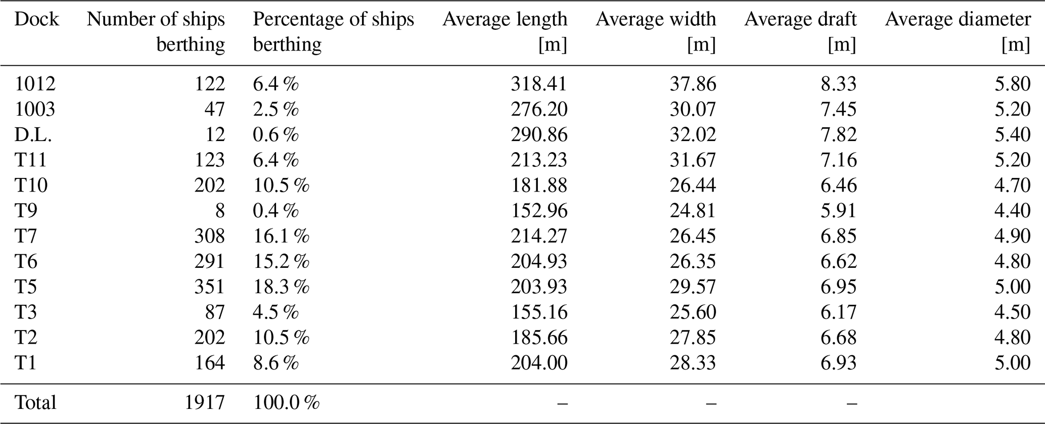
Table 1 shows the results of the traffic analysis within the port of Genoa for 2017 conducted using the daily traffic data provided by Stazioni Marittime SpA. The annual traffic is generally regular, and its frequency varies from basin to basin and depends on the season. Generally, the busiest docks are T5, T6, and T7, which account for almost 50 % of the total traffic. They follow an approximate daily frequency all year round, whereas the wet basins towards the end of the port, which mainly serve cruise vessels, show an evident seasonality, probably related to the Mediterranean cruise season (few and irregular passages from January to May and then regular and a much increased frequency from June to October or November).

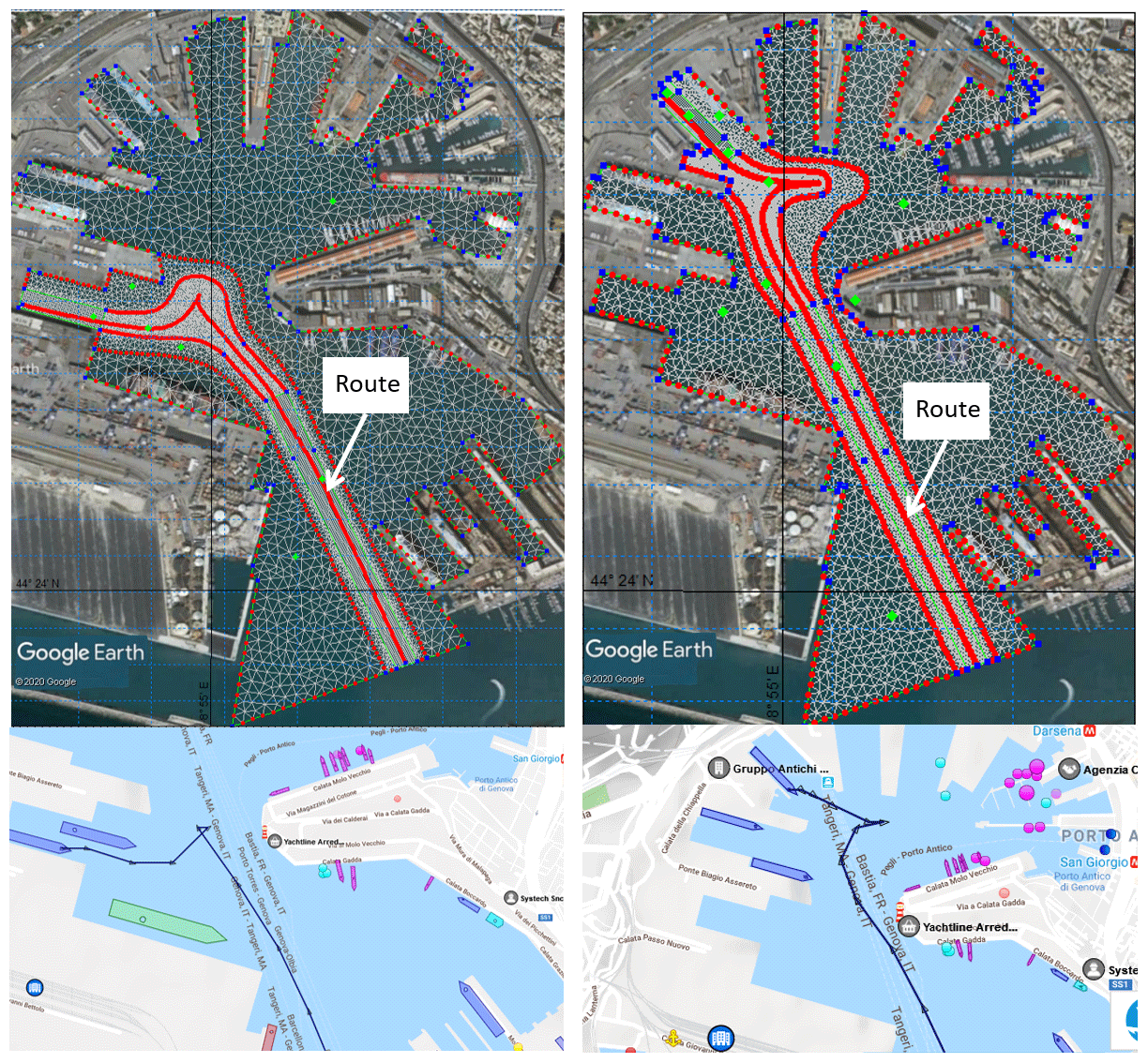
Figure 4 Model domain and computational grids for docking routes for the T1 (left panel) and T10 (right panel) docks. In the lower panels, the corresponding actual routes are shown. Land background of the upper panels is from © Google Earth.

Table 1 Analysis of ship traffic in the port of Genoa for the year 2017 and the main characteristics of the ships representative of each dock. The ships' length, width, draft, and propeller diameter values are expressed in meters.

In the vertical, the model is resolved over 10 evenly distributed sigma layers. The resulting layer depths vary from approximately 1 m in the berthing areas to approximately 2 m in the pits and in the areas closer to the port's entrance.

4.1.1 Propeller jet velocity

The propellers' maximum jet velocity was calculated based on the Code of Practice of the Federal Waterways Engineering and Research Institute (Abromeit et al., 2010) and the PIANC Report no. 180 (MarCom WG 180, 2015), taking the German approach. The relevant parameters for the calculations are shown in Fig. 1. The maximum velocity V₀ after the jet contraction generated by the propeller is developed along its axis. For unducted propellers, we use Eq. (1a) for the propeller ratio J=0 (ship not moving) or Eq. (1b) for J≠0 (moving ship):

$$\begin{array}{}\text{(1a)}& {\displaystyle }{V}_{\mathrm{0}}=\mathrm{1.60}{f}_{\mathrm{n}}{n}_{\mathrm{d}}D\sqrt{K_T}\text{(1b)}& {\displaystyle }{V}_{\mathrm{0}j}={\displaystyle \frac{\sqrt{\left(J^{\mathrm{2}}+\mathrm{2.55}{K}_{Tj}\right)}}{\sqrt{\mathrm{1.4}\frac{P}{D}}}}{V}_{\mathrm{0}},\end{array}$$

where n_d [1 s⁻¹] is the design rotation rate of the propeller; f_n is the factor for the applicable propeller rotation rate (nondimensional); D is the propeller diameter [m]; K_t or K_tj is the thrust coefficient of the propeller (nondimensional) in the case of non-motion or motion of the ship, respectively; and P is the design pitch [m]. Typical values for f_n are 0.7–0.8 during maneuvering activities, and the $P/D$ ratio can be assumed to be approximately equal to 0.7. K_t or K_tj can be estimated through Eqs. (2a) and (2b), according to the state of motion of the ship:

$$\begin{array}{}\text{(2a)}& {\displaystyle }{K}_{\mathrm{t}}=\mathrm{0.55}{\displaystyle \frac{P}{D}}\text{(2b)}& {\displaystyle }{K}_{\mathrm{t}j}=\mathrm{0.55}{\displaystyle \frac{P}{D}}-\mathrm{0.46}J.\end{array}$$

The propeller ratio J depends on a wake factor w, which varies from 0.20 to 0.45 (nondimensional), and on the velocity of the ship according to Eq. (3):

$$\begin{array}{}\text{(3)}& J={\displaystyle \frac{v_{\mathrm{s}(\mathrm{1}-w)}}{nD}}.\end{array}$$

As proposed by Hamill (1987) and further described by Lam et al. (2005), the downstream propeller-induced jet is divided into a zone of flow establishment (closer to the propeller) and a zone of established flow (further downstream). The resulting velocity V₀ used in the model to calculate the corresponding discharge and momentum sources is considered as the maximum velocity at the beginning of the zone of the established flow.

As we had no direct information about the size of the ships' propellers, we referred to the specific literature. For the propellers of the Ro-Ro ferries that typically serve docks T1, T2, T3, T5, T6, T7, T9, T10, and T11, we referred to report no. 02 of the “Mitigating and reversing the side-effects of environmental legislation on Ro-Ro shipping in Northern Europe” project (Kristensen, 2016), implemented by the Technical University of Denmark (DTU) and HOK Marineconsult ApS. According to this study, the relationship between the draft and the diameter of the ferry's propeller is given by Eq. (4):

$$\begin{array}{}\text{(4)}& D_{\mathrm{prop}}=\mathrm{0.56}\times H_{\mathrm{draft}}+\mathrm{1.07},\end{array}$$

where D_prop is the propeller's diameter [m], and H_draft is the maximum draft of the ship [m]. This relation is not valid for cruise ships, as they typically have larger propellers. For this type of ship, which serves docks 1012, 1002, and partially D.L. and T11, we directly referenced operators in the passenger ship design sector, and double-checked the information using the formulas from Eq. (4) and Eq. (5), which is also valid for double-propeller passenger ships. This qualitative analysis provided the diameters presented in Table 1.

$$\begin{array}{}\text{(5)}& D_{\mathrm{prop}}=\mathrm{0.85}\times H_{\mathrm{draft}}-\mathrm{0.69}\end{array}$$

The water discharge was obtained by combining the diameter of the propeller and the intensity of the jet, which was discretized into a certain number of smaller discharges associated with various smaller sources of momentum in the numerical model. Thus, we realistically represented the propeller. The distribution of volume and momentum sources follows a spatially Gaussian (normal) distribution with a discretization step of 0.5 m and a constant rotation rate of the propeller.

Figure 5 shows the propeller-induced jet in the hydrodynamic model. Panel a represents the plan of dock 1012, where a large cruise ship is departing. The solid line in Fig. 5a is the location of the vertical transect shown in Fig. 5b, representing the jet velocity in the plane xz. The dashed line in panel a represents the trajectory followed by the axis of the departing ship, and the associated jet's velocity in the yz plane is shown in panel c. Although the horizontal resolution is nonoptimal in terms of propeller representation, the resulting jet appears extremely realistic both in the transverse and longitudinal directions.

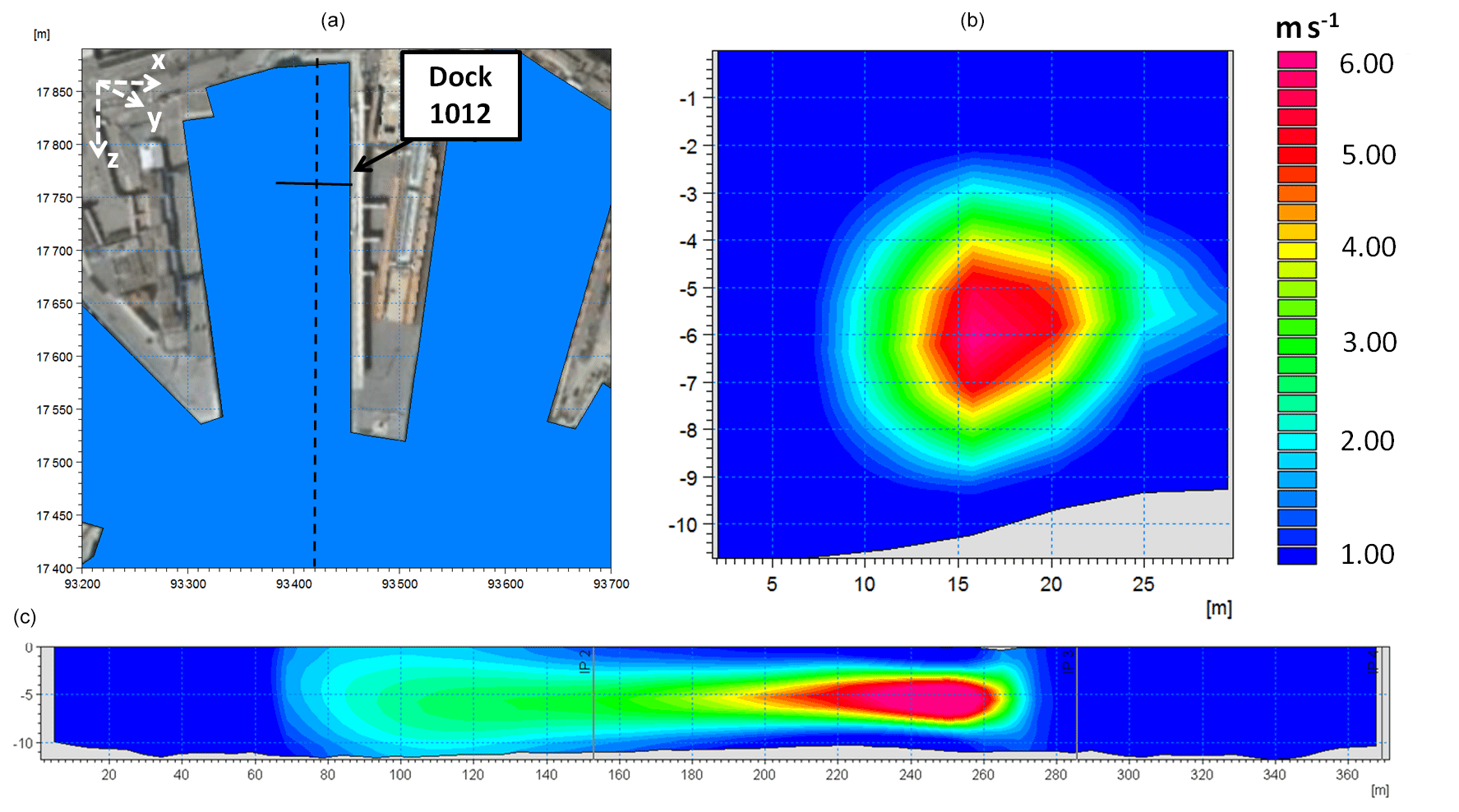
Figure 5 Representation of the propeller-induced jet of the most representative ship departing from dock 1012. (a) Plan view of the ship's departure: the dashed line represents the trajectory followed by the axis of the undocking ship, and the solid line represents the position of the vertical transect shown in panel (b). (b) Vertical transect showing the jet-induced velocity in the xz plane (propeller's plane). (c) Transect of velocity along the propeller's axis (yz plane). Velocities are in meters per second (m s⁻¹). Land background from © Google Earth.

To preserve the water mass budget, we associated a sink to each source. Sinks are prescribed in terms of negative equivalent discharge (m³ s⁻¹) in the grid cell adjacent to that hosting the source, in the direction of the ship motion (sinks precede corresponding sources).

The choice of the vertical and horizontal resolutions of the hydrodynamic model were the result of a thorough sensitivity analysis of the grid's cell dimensions. We assumed that the most appropriate resolution for the model allows the maximum (jet centerline) current produced by the combined discharge and momentum sources in the model to reach the input maximum velocity of V₀. For the sensitivity analysis, we considered a 4 m diameter propeller with a rotation rate of 2 rps (revolutions per second) at full power. According to Eq. (1b), this configuration results in a V₀ of approximately 6 m s⁻¹ at the depth of the propeller's axis once the jet is fully developed. We set up an experimental configuration domain 100 m wide and 500 m long. We tested horizontal resolutions of 20, 10, 5, 2, and 1 m, whereas we considered two configurations for the vertical: 10 and 20 layers in a constant bathymetry of 20 m. The input value of the jet current to the model was 6 m s⁻¹.

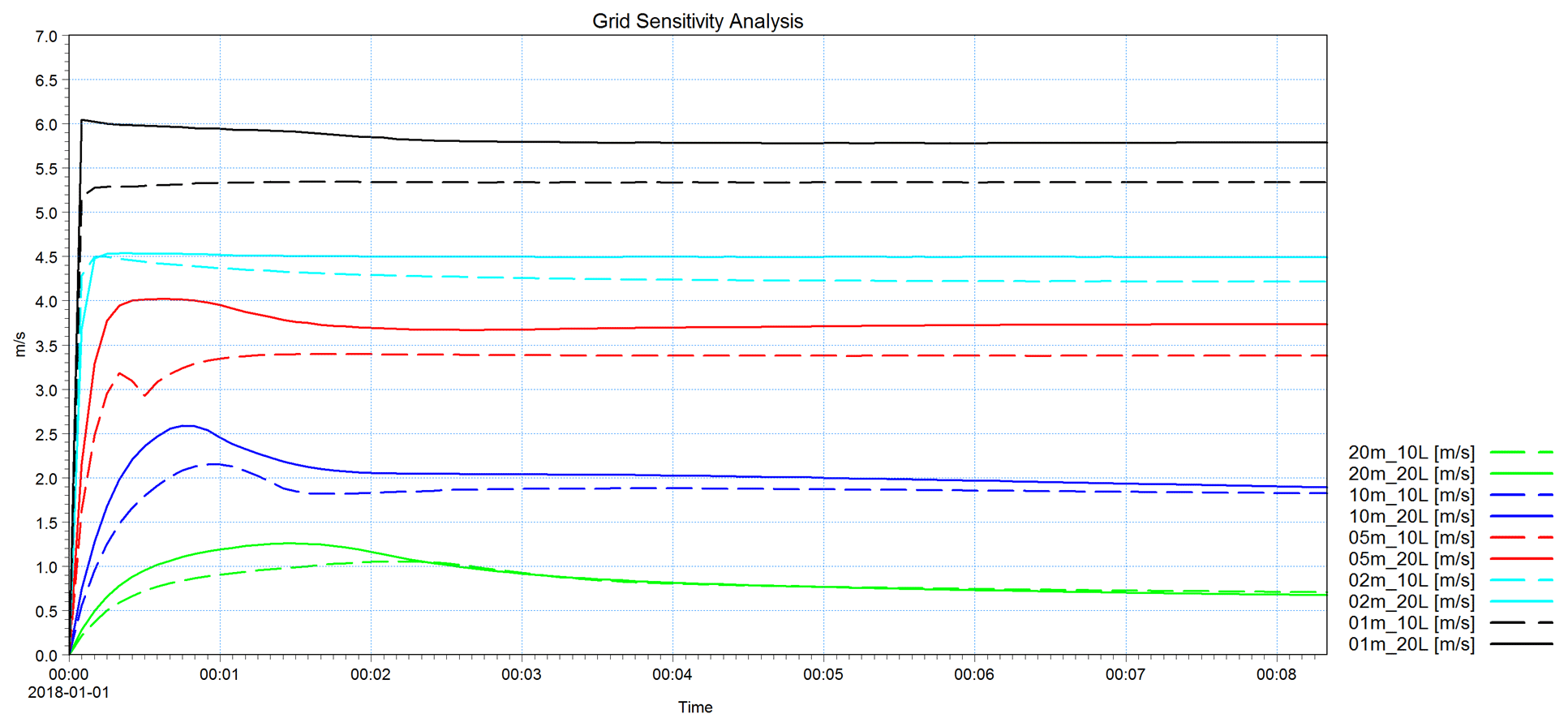
Figure 6 Model grid sensitivity analysis to the cell's dimension. The different colors correspond to different horizontal resolutions. Dashed lines indicate the configurations with 10 layers, and solid lines indicate those with 20 layers.

Figure 6 shows the sensitivity analysis of the grid resolution. The resulting velocity at the propeller's axis is proportional to the resolution, both in the vertical and the horizontal: the higher the resolution, the higher the resulting velocity. The most appropriate grid is that with a 1 m resolution and 20 vertical layers, which is the only configuration of the model that allows the jet to reach the maximum speed imposed as the input. However, this configuration would require approximately 1 year of computational time to run the 24 simulations implemented in this study in the same computational configurations, which is obviously unrealistic. Therefore, we sought a compromise between acceptable computational demand and realistic resulting velocity. The final configuration took 5 m as the horizontal resolution and 10 vertical levels. As these resolutions did not allow for the complete development of the current speed, we introduced a correction to the input velocity of each simulated vessel by increasing it by the necessary amount to reach the empirically calculatedV₀. This involved considerable additional time for manual calibration.

4.1.2 Forcing and boundary conditions

Due to the nature of the focal processes, we only account for the force of the propellers of the vessels. The jet induced by its motion is of an order of magnitude of several meters per second in the area surrounding the blades and when unconstrained it has a length of influence of at least 40–50 times the propeller's diameter behind the ship (Verhei, 1983). This is also an important source of toe scouring in the presence of a quay wall (Hamill et al., 1999). Natural forcing such as wind, density gradients, or tides are one to two orders of magnitude smaller and can, therefore, be neglected without introducing errors that can potentially affect sediment resuspension from the bottom. However, the Bernoulli wake may be responsible for currents of comparable intensity (Rapaglia et al., 2011), although smaller, and can be a forcing source in the system. In any case, we do not consider this due to technical complications and time constraints. Including such a process in further developments and analyzing its impact on the overall dynamics of ship-induced sediment transport would be of interest. Our final results prove satisfactory, suggesting that the governing processes for these dynamics are associated more with propeller-induced currents than with the motion of the ship itself, likely due to the limited speeds of vessels in this inner part of the harbor and to the relatively large volume of water available for each passing vessel.

The boundaries of the hydrodynamic domain are the docks around the basin and the port entrance, which is the only open boundary. Here, we imposed a Flather condition (Flather, 1976), assuming constant zero velocities and levels. This allowed us to minimize the boundary effects, albeit with some interference between the flux and the boundary line (not shown). However, due to the distance between the open boundary line and the berthing areas, such effects do not influence the results of the study. A zero normal velocity was imposed along the closed boundaries.

4.2 The sediment transport model

The hydrodynamic model was coupled with a sediment transport model – MIKE 3 MT FM – valid for fine-grained and cohesive sediment (diameter smaller than 63 µm; Lisi et al., 2017). This is the main type of sediment in the port of Genoa and is particularly relevant in terms of erosion, transport, and further deposition, as its small particle dimension and light weight rapidly lead to its resuspension and advection around the basin.

The equations of the mud transport model are based on the advection and dispersion (AD) of the sediment concentration along the water column and are detailed in Appendix B. The AD equation is solved using an explicit, third-order finite difference scheme called ULTIMATE (Universal Limiter for Transient Interpolation Modeling of the Advective Transport Equations; Leonard, 1991).

The model consists of two areas: a water and a seabed environment. The seabed is represented through a multi-bed layer and multi-fraction approach in which the layers can exchange mass and only the top level is active, thereby making it available for erosion. The different layers are defined by the proportions of sediment in their composition, the degree of consolidation of the sediment within each layer, and the thickness of the single layer. The sediment proportions are described through their associated physical characteristics, and are eroded and deposited proportionally to their concentration both in the bed texture and along the water column. Flocculation processes occur in the water environment of the model when a certain concentration threshold is exceeded (here assumed to be equal to 0.01 g L⁻¹), whereas settling is hindered at a threshold of 10 g L⁻¹, according to the definition of Winterwerp and Kesteren (2004). The deposition of the sediment is based on a Teeter profile (Teeter, 1986), and the threshold for deposition used was 0.07 N m⁻². The sediment grain diameter is defined through the associated settling velocity, based on Stokes' law. In the interface between the water and the bottom, the sediment may be eroded, as proposed by Partheniades (1965) for consolidated sediment or by Parchure and Metha (1985) for soft or unconsolidated sediment. In both cases, the sediment is eroded and injected into the water column when the shear stress resulting from the current, the wave action, or a combination of both exceeds a certain critical value. We do not consider waves, as our focus is inside the port.

The specific equations and parameterizations referred to in the sediment model are summarized in Appendix B.

Sediment characteristics

Three sediment surveys were conducted between June 2009 and July 2010. Table 2 presents the results of the surveys in terms of percentage and class of sediment per survey (right and center column, respectively). Given the nature of our study, our focus is on mud and fine sand; thus, grains coarser than 2 mm were not considered.

Table 2 Sediment size data inside the port (see the station identified using the red dot in Fig. 2). Three different surveys were carried out between June 2009 and July 2010. (All times are given in local time.)

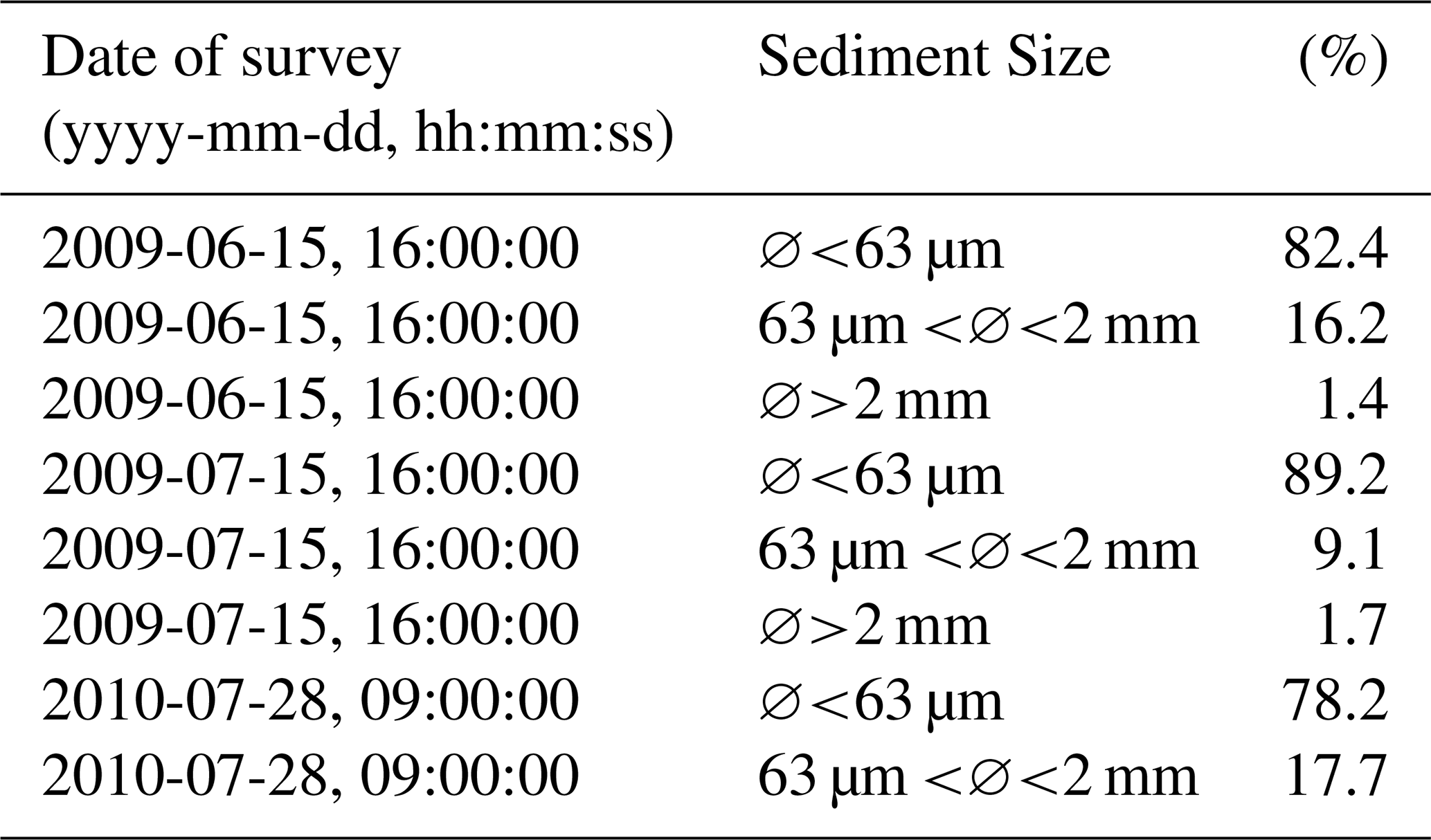
We assumed that the proportions of the samples with ∅<63 µm were composed of two grain sizes with diameters of 30 and 50 µm, respectively, whereas for the observed components with diameters in the range of 63 to 2 µm, we assumed 100 µm to be representative.

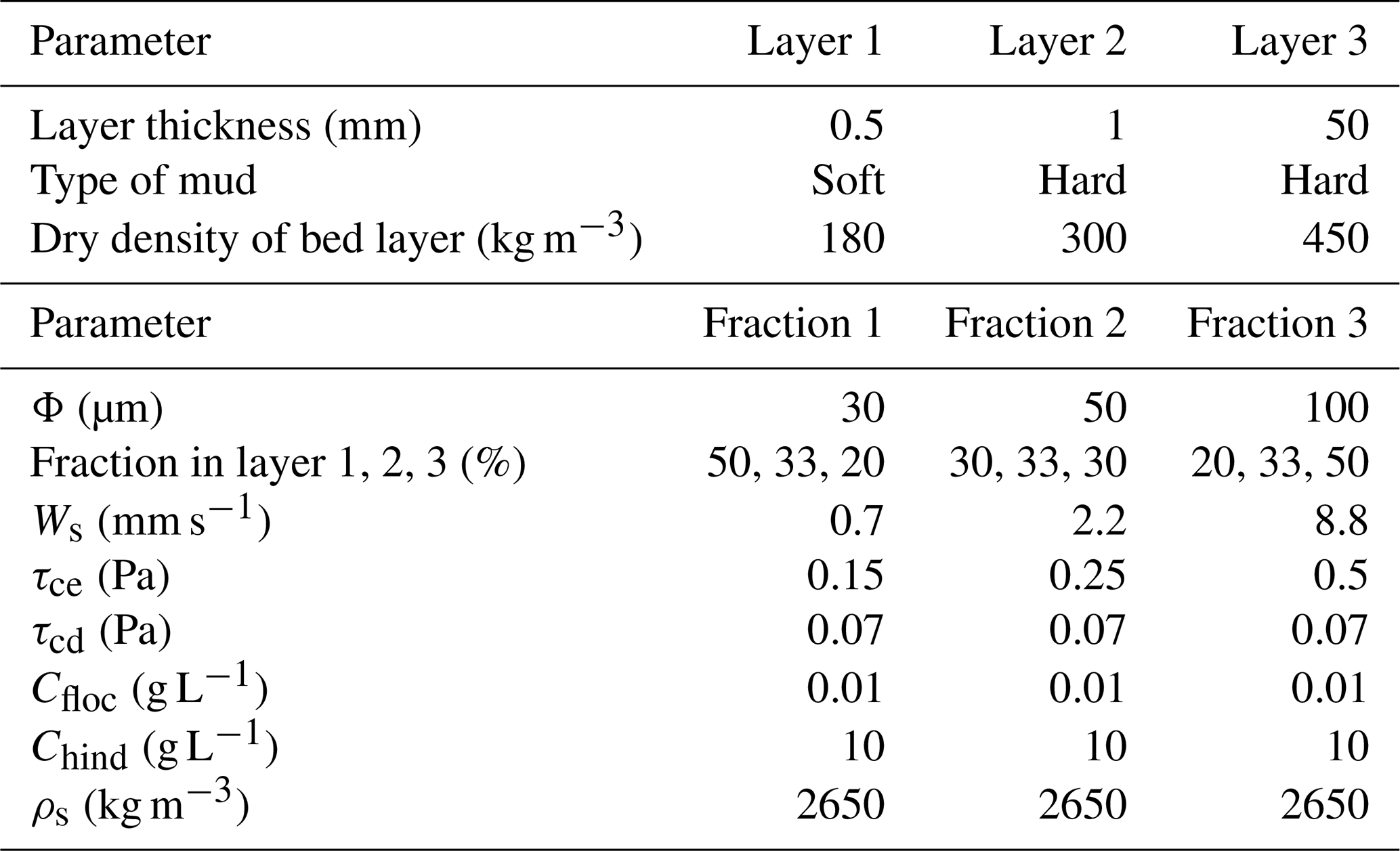
The degree of consolidation of the seabed is both time- and depth-dependent. The upper layer, which mostly contributes to the flux of resuspended sediments into the water column, is composed of freshly deposited sediment as it is subject to continuous reworking. The lower layers are more consolidated, and the degree of consolidation increases by depth. This vertical gradient in seabed properties is enhanced in a port environment, as the upper layers are continuously influenced by the propeller-induced jets (several times per day); hence, multilayer modeling of the seabed is appropriate. Teisson et al. (1993) and Sandford and Maa (2001) also took this approach. A single layer bed representation would imply an overestimation of the bed's erodibility (soft mud and thus easily reworked), resulting in unrealistic further overestimations of sediment erosion and concentration along the water column. Therefore, a multilayer representation of the seabed is required to account for the transition from unconsolidated to consolidated material. Amorim et al. (2010) used a two-layer approach to model the seabed with MIKE software, simulating the sediment transport in the navigation channel of the port of Santos. However, as they suggested, a two-layer representation of the seabed may produce an unrealistically abrupt transition between erodible and hard bed layers; therefore, in order to consider a gradual transition from freshly deposited to consolidated material, three bed layers were defined here, representing the freshly deposited, slightly consolidated, and fully consolidated sediments. The percentage of the fine particles in the sediment texture was assumed to decrease proportionally to the depth of the layers. Thus, the first layer contained 80 % of fine grains (50 % of grains of ∅=30 µm and 30 % of ∅=50 µm) and 20 % of coarse grains (∅=100 µm), whereas the third layer contained 50 % of coarse grains (∅=100 µm) and 50 % of fine grains (20 % of grains of ∅=30 µm and 30 % of ∅=50 µm). In the mid layer, an even distribution was assumed among the three. The thicknesses of the three layers are 0.5, 1, and 50 mm at the beginning of each scenario. The first layer is composed of very soft mud, as it is the result of the newly deposited and finer mud. The other two layers are more consolidated and thicker, as they are less easily eroded and are shielded by the upper layers. The different layers and fractions of sediment that characterize the bottom enabled us to represent the port bed in a complex and comprehensive way and to include the various degrees of consolidation of the layers and the resulting responses to shear stress.

The main characteristics of the layers and sediment proportions implemented in the sediment transport model are presented in Table 3.

Finally, sediment input may also potentially come from six minor streams that flow into the port area. These have very modest basins of approximately 1 km² on average, and they have been ceiling-covered for many years, so they now act more as sewage collectors than natural streams. Their contribution to the sedimentary dynamics of the port of Genoa has been estimated, and the annual sediment supply to the port basin from each stream has been evaluated based on the method proposed by Ciccacci et al. (1989). The estimated sediment contribution was only a few hundred cubic meters per year in the worst case, which corresponds to a contribution to the wet basins of a few millimeters of annual accumulated sediment from the surrounding river inlet. This level of solid matter has not been considered in the model, as the erosional and depositional processes induced by the propeller activity are higher by 1 or 2 orders of magnitude.

Table 3 Summary of sediment characteristics as implemented in the mud transport model.

5 Results and discussion

The main results of the hydrodynamic and sediment transport model are presented in this section. Due to the large number of simulations carried out, only those regarding two docks are shown. However, the current and sediment concentration results corresponding to the other simulations are qualitatively similar. We focus on the simulations of docks 1012 and T7. dock 1012 is particularly important as it hosts the largest passenger vessels operating in the port, whereas dock T7 has a high frequency of passages.

Figure 7a and b show the propeller-generated current in the bottom layer and at the depth of the propeller's axis, respectively, and Fig. 7c and d show the corresponding resulting suspended sediment concentration in the same layers during the departure of a cruise vessel from dock 1012. The characteristics of a vessel representative of the traffic in the dock are given in Table 1. When departing, the engine operates close to full power, which we assume results at a rotation rate of 2 rps for the propeller. This induces a maximum velocity at the depth of the propeller axis close to 9 m s⁻¹, which is damped to approximately 2 m s⁻¹ on the bottom of the berthing basin along the vessel's route. This intense jet is deflected to the left due to the head wall of the berthing basin, which constrains the flow and induces a cyclonic eddy that is well-developed along the whole water column. The cone-like envelope of the jet in the vertical plane, as illustrated in the theoretical scheme of Fig. 1, can be observed in Fig. 7a and b, which refer to the same example: the influence of the propeller on the bottom occurs several tens of meters behind the propeller's position, and the velocity at the bottom is much reduced. The induced eddy in the wet basin acts as a trap for the eroded sediment, which enters the cyclonic gyre (or anticyclonic gyre in the case of departure from the opposite dock) and tends to deposit in the middle of the basin, where the fluxes progressively decrease. The position of the eye of the cyclone evolves parallel to the docks' longitudinal walls and induces the sediment trapped inside the gyre to sink along the longitudinal axis of the wet basin. Such dynamics occur similarly for all the horseshoe-shaped wet basins, inducing accumulation along the central portions. The resuspended sediment may reach very high concentrations of up to several hundreds of milligrams per liter in the bottom layers, depending on the different specific characteristics of the sediment texture (such as grain size, level of consolidation, and availability to erosion) and of the vessel (such as dimensions of the propellers, rotation rate, and draft).

Various hydro and sediment dynamics occur during the inbound phase of vessels maneuvering inside the port. Most of the maneuvering operations (i.e., when vessels rotate within a turning basin and proceed backwards to the docks) occur in the turning basins denoted by the dashed circles a and b in Fig. 2. The engines operate at high power when starting the maneuver to allow for the rotation of the ship. The vessel's longitudinal axis then rapidly changes direction (from tens of seconds up to a few minutes) and can span wide angles, depending on the specific maneuver. The propeller-induced jet follows the same rotation along the horizontal plane, resulting in a fan-like distribution of directions for the associated currents. Such operations are realistically represented by the model, as shown in Fig. 8, which refers to the berthing of the vessel representative of dock T7. The currents shown in the figure are those associated with the propeller's axis during four different moments of the turning maneuver. Each panel refers to successive time intervals of approximately 100 s. These successive instants are presented in the following order: upper-left panel, upper-right panel, lower-left panel, and lower-right panel. In the lower-right panel, the propeller has already changed rotation direction and the vessel is now proceeding backwards. Thus, the induced current jet is heading towards the center of the port and pushing the sediment towards this area. The simultaneous seabed activity is shown in Fig. 9. Although the jet-induced currents are much weaker at the seabed than those at the depth of the propeller's axis, they are still significant and may reach intensities of up to 1 m s⁻¹, depending on the local bathymetry.

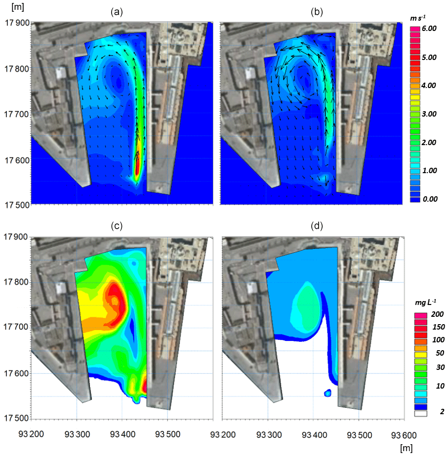
Figure 7 Results of the numerical models. (a, b) Current intensity and direction in the bottom layer and (b, d) in the layer corresponding to the axis propeller. (c, d) Resulting suspended sediment concentration (SSC, mg L⁻¹) in the same layers as in panels (a) and (b). The images refer to the undocking of the cruise vessel representative of dock 1012. Land background from © Google Earth.

The current distribution at the seabed is much more chaotic than at the propeller's axis depth. This area of the port corresponds to the natural pit (which reaches approximately 22 m below the surface in the deeper part) in which the material dredged from the accumulation areas is often dumped during the sea bottom maintenance activities. The dashed line shown in the lower-right panels of Fig. 8 and Fig. 9 refers to the transect presented in Fig. 10, for the same instant (i.e., when the vessel has ended the maneuver in circle b and is approaching dock T7 backwards).

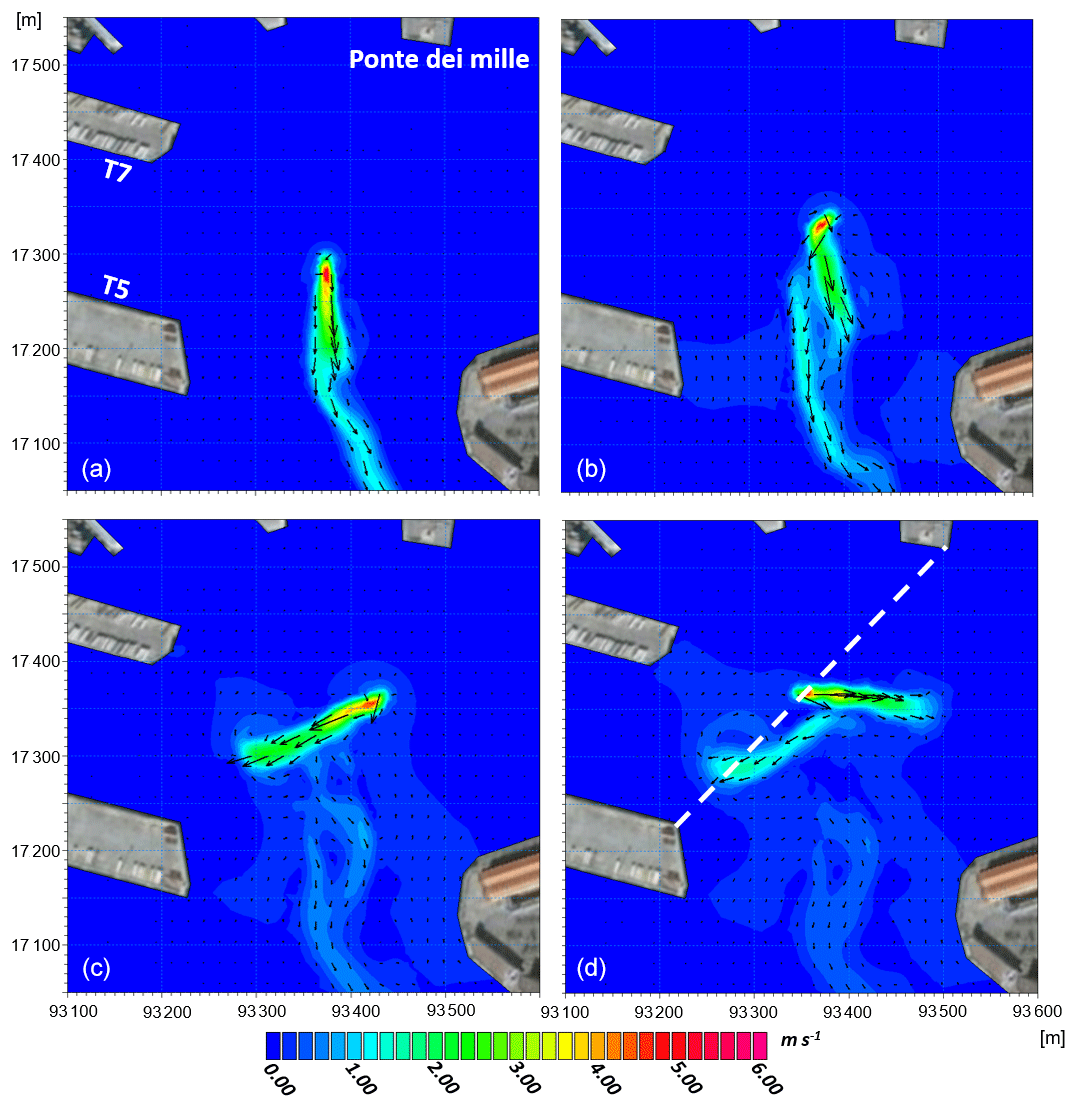
Figure 8 Results of the hydrodynamic model at the depth of the propeller's axis. Each panel refers to a time interval of approximately 100 s from the previous panel. The temporal order of the panels is as follows: (a), (b), (c), and (d). The images refer to docking maneuvers of the Ro-Ro vessel representative of dock T7. Land background from © Google Earth.

A combined analysis of Figs. 8, 9, and 10 helps us understand the dynamics occurring in turning basin b during the maneuvers when approaching docks T5, T6, and T7, and particularly the overall sediment dynamics of the entire port, as these three docks account for approximately half of the entire passenger traffic. The propeller-induced velocities at the bottom of the natural pit during turning maneuvers are variable and may exceed 1 m s⁻¹, which is a significant current intensity that can entrain and move a large amount of sediment. The resulting resuspended sediment concentration may reach values exceeding 50–60 mg L⁻¹, as shown in Fig. 10b. Once resuspended from the pit, the sediment is advected by the jet-induced complex field of currents of Figs. 8 and 9. This area is typically refilled with freshly dredged material resulting from the seabed maintenance activities; thus, the propeller-induced currents on the bottom have an enhanced erosion effect on the unconsolidated material and can rapidly nullify the benefit of the dredging operations. Hence, the results of the simulations suggest avoiding the use of the natural pit as a dumping area for the resulting material, and they confirm that integrated modeling can be an effective tool for simulating the processes and mechanisms related to sediment transport as well as for the optimized planning of maintenance activities.

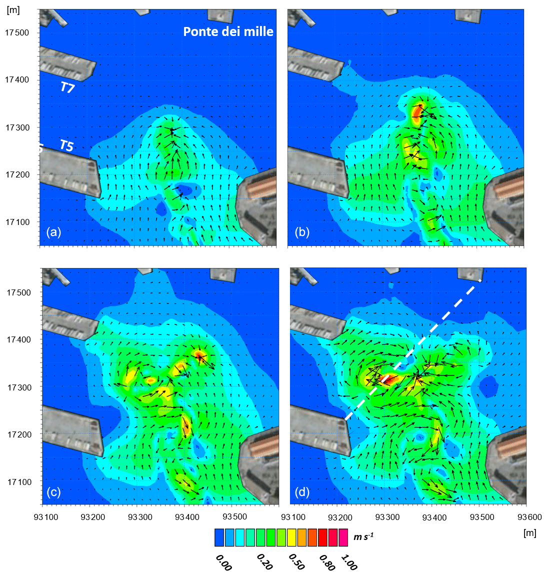
Figure 9 Results of the hydrodynamic model in the bottom layer. Each panel refers to a time interval of approximately 100 s from the previous panel. The temporal order of the panels is as follows: (a), (b), (c), and (d). The images refer to docking maneuvers of the Ro-Ro vessel representative of dock T7. Land background from © Google Earth.

The impact of the marine traffic on the bed thickness is illustrated in Fig. 11, which presents the erosion and deposition maps resulting from the simulations of one departure (left column) and one arrival (right column) of the representative passenger vessels of docks 1012 (top row) and T7 (bottom row). Blue represents areas of erosion, and red represents the accumulation of the sediment after an interval of time long enough for the resuspended sediment to completely settle. The left column Fig. 11 shows that a considerable amount of material tends to be eroded from the bases of the docks during the vessel's departure and then settles in the center of the mooring basins. This mechanism is clearly related to the vessel's departure (left column) rather than its arrival (right column). The erosion underneath the vessel's keel along its trajectory is evident, both during departure and arrival, thereby supporting previous experimental findings (Catells et al., 2018). The magnitude of the erosion and deposition of a single vessel's passage is of the order of a few millimeters in the areas most influenced by the vessel's activity.

Such an impact can become a real threat to the continuity of operations in large and busy ports such as Genoa over medium to long timescales. The few millimeters of accumulation and erosion can become several tens of centimeters after a few thousand annual passages. For the sake of completeness, the results of the impact on the bed thickness due to the activity of the other vessels not shown in the main body of the text are presented in Appendix C.

Based on the traffic analysis in Table 1, we projected each single marine passage to a 1-year duration and superimposed the effects of erosion and deposition of vessels that are representative of all of the passenger docks. Thus, we were able to reconstruct the annual port seabed evolution for the year of 2017. The effects of the single passages were weighted by the specific occurrences of that year, which resulted in 24 maps (one for each docking and one for each undocking), and the results were integrated to obtain a final map.

As the trajectories for reaching a dock (or departing from it) vary slightly from passage to passage, a Bartlett spatial filter was applied to the integrated results using the values of 4, 2, and 1 as weights. Figure 12 presents the results of this analysis. In the left panel, the results from the modeling system in terms of annual erosion (blue) and accumulation (red) are shown, and in the right panel, the observed seabed evolution is shown. The observed map was reconstructed using the outcomes of two bathymetric surveys carried out in the May–June 2017 and March–June 2018 periods. The difference in the bathymetries of the two surveys resulted in the evolution of the seabed during the approximate 1-year period, except for dredging operations. We indicated the areas where the most significant dynamics took place on the maps using numbers.

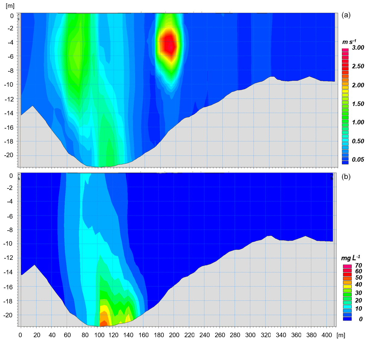
Figure 10 (a) Velocity intensity (in m s⁻¹) and (b) sediment concentration (in mg L⁻¹) along the transect from the head of Ponte Assereto to the head of Ponte dei Mille.

The area between the heads of Ponte dei Mille and of Molo Vecchio, identified as 1 in Fig. 12, was dredged during the October–December period in 2017, and approximately 15 000 m³ of solid material was removed and dumped into the natural pit of the port, as indicated by the number 5. Thus, what, at first sight, appears to be an area of erosion due to vessel traffic – area 1 in the right panel of Fig. 12 – is actually an area of accumulation, which is confirmed by the fact that dredging operations were conducted. Similarly, the accumulation observed in area 5 (right panel of Fig. 12) is not the result of the induced action of the propellers but of the accumulation of the sediment dumped after the maintenance dredging operations. The model results are in total agreement with these dynamics. As discussed above, the material resuspended during vessels' maneuvers is likely pushed towards area 1 in the phase during which the vessels approach the docks backward. Conversely, area 5 is partially an area of erosion, as evidenced by the model. The freshly deposited material during dredging operations is thus rapidly resuspended.

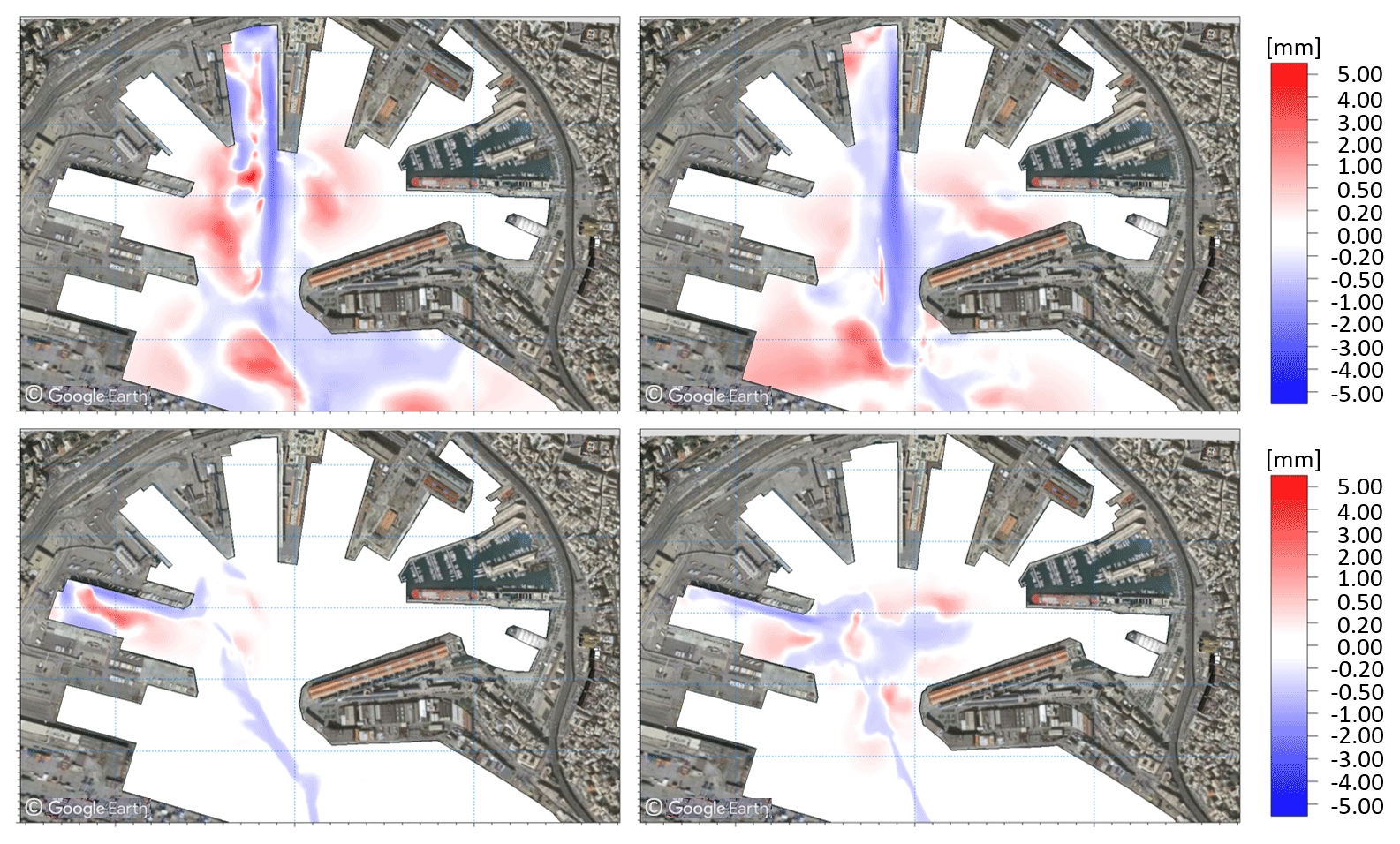
Figure 11 Erosion and deposition maps resulting from one departure (left column) and one arrival (right column) of the representative passenger vessels of docks 1012 (top row) and T7 (bottom row). Land background from © Google Earth.

Area 1 accounts for approximately 30–40 cm yr⁻¹ of accumulated material, with local maxima of up to 50 cm yr⁻¹. Similar values were estimated through years of managing experience by the personnel of Stazioni Marittime S.p.A (Edoardo Calcagno, personal communication, 2019).

The central portions of the wet basins marked with number 2 in Fig. 12 are areas of deposition, mainly due to the departure phase of the ships. Again, the model can efficiently reproduce both the accumulation along the central parts of the basins, where it may reach 20 cm yr⁻¹ or even more, and the erosion along the walls of the docks. Here, the propellers' erosive action may result in stability problems for the docks, particularly along the walls of dock 1012, where the biggest cruise vessels operate.

The erosion underneath the vessels' typical routes (i.e., from the entrance to approximately the center of the port) is also well represented by the model (identified using the number 6 in Fig. 12). The model and the observations also exhibit good agreement in the deposition area (number 7), where a local gyre forms and entraps the suspended sediment. Finally, areas 3 and 4 are also subject to deposition, and qualitative agreement between the model and the various bathymetric surveys is evident from Fig. 12. The erosive print observed in the survey under these areas is most likely due to activities related to cargo vessels approaching and departing from dock Calata Sanità. These vessels were not the focus of our study, and Calata Sanità only operates container ships; thus, the model does not include the marine traffic in this area.

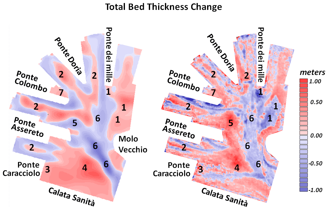
Figure 12 Annual erosion and deposition map reconstructed on the basis of the hydrodynamic and sediment transport simulations for the year 2017.

In general, the observed and the modeled annual evolution of the port seabed show very good agreement, which confirms the reliability and robustness of the hydrodynamic and sediment transport model and demonstrates the potential importance of an integrated modeling approach in optimizing the management of port activities.

The assumption of unvarying initial bathymetry conditions in the different scenarios deserves some additional consideration, as it undoubtedly introduces some inaccuracy into the results. This approach does not consider the real order of vessels' passages or the impact that the evolving seabed has on the hydrodynamics and sediment transport simulations. In particular, the variable clearance distance between the propeller's tip and the seabed due to the evolving erosion and deposition processes is not considered, although this will increase the differences over time. However, the complexity of the system requires the introduction of several approximations, such as the dimension and rotation rates of the propellers, the typology and distribution of the sediment, the layering of the sea bed, the shear stress for erosion and deposition, or the constant initial bathymetry. A solution for the bathymetry issue could be to implement the system in operational mode and, thus, continually update the initial bottom boundary conditions through the simulation iterations. However, this was not realistic in terms of computational effort and was beyond the scope of the study, which was to identify areas of erosion and deposition in the port and to evaluate the order of magnitude of the corresponding evolution rates to support the port management. Nevertheless, if we consider the most significant variation in the seabed and the typical propeller-induced bottom velocities, which are of the order of 50 cm (Fig. 12) and 1–2 m s⁻¹ (Figs. 7, 9, and 10), respectively, the resulting bottom shear stresses are of the order of 2–4 N m⁻². Such values are orders of magnitude larger than the typical critical shear stress for the deposition and erosion of freshly deposited fine sediments (of the order of 0.07–0.15 N m⁻², respectively), suggesting that variations in the bottom shear stresses due to a change in the clearance distance of the propeller's tip of the order of 50 cm (a conservative estimate) would not have a significant impact on the mobility of the sediments. Consequently, such differences would not imply substantial variations in the erosional and depositional processes and patterns.

6 Summary and conclusions

The impact of marine traffic on the seabed of the passenger port of Genoa was investigated through numerical modeling. The combination of a very high-resolution, non-hydrostatic, circulation model (MIKE 3 HD FM) with a sediment transport model (MIKE 3 MT FM), based on unstructured grids on the horizontal and on sigma levels on the vertical, enabled us to reconstruct the annual evolution of the port seabed. The final results of the modeling, in terms of maps of erosion and deposition inside the basin, were qualitatively supported by observational evidence. Our approach was to simulate only one arrival and one departure from each dock of the port and to analyze the impact of a single marine passage on the seabed in terms of sediment concentration, motion, and distribution.

From the traffic analysis in the port for a typical year (2017), we could obtain the detailed situation of the number of arrivals and departures for each dock as a starting point for the study. By superimposing the effects of single vessels weighted for the annual number of passages of the most representative vessel operating on each dock, an annual map of erosion and deposition was reconstructed and validated on a semiquantitative basis by comparison with various bathymetric surveys for the same period.

In general, the simulations showed that the velocity intensities on the bottom induced by propeller-generated jets can reach almost 2 m s⁻¹, and mainly depend on the dimensions of the propellers, the rotation rate, and the distance between the propeller and the bottom. Such velocities may reach up to 8–9 m s⁻¹ at the propeller's axis depth and penetrate horizontally through the water for long distances, up to at least 40–50 times the propeller's diameter. The bed shear stresses induced by these velocities as well as the propeller jet-induced entrainment, mobilize and resuspend large amounts of the fine and less compacted sediments present inside the port. Fine proportions with lower fall velocities tend to remain in suspension for longer periods of time, resulting in the creation of sediment plumes.

Our findings showed how significant these deposition rates can be in a densely operated port, reaching values of several tens of centimeters per year in specific areas.

Our approach enabled us to minimize the computational time and also decompose the overall complex view of sediment transport of the entire port into several simpler views. Consequently, we were able to analyze the specific hydro and sediment dynamics for each dock and vessel, and to identify specific routes responsible for particularly serious erosion and accumulation, as historically reported by the management authorities of the port operations and traffic. The range of current intensities induced by the propeller action was identified along the water column, and this can be further used as a sound and scientifically based benchmark value for potential defensive actions on the seabed and port structures in order to guarantee the ongoing full operability of the port.

The most significant mechanisms for the port's hydro and sediment dynamics that occur during vessel passages were identified and the subsequent analysis identified how and why specific areas are subject to erosion and other areas are subject to deposition as well as the extent of these mechanisms. In particular, the mechanism of ongoing erosion along the docks' walls and of deposition along the central portions of the mooring basins were identified and explained, along with the ongoing deposition process in the area between the heads of Ponte dei Mille and Molo Vecchio. Identifying and reproducing this process for the port managers was particularly important, as it occurs at a very significant rate of up to 40–50 cm yr⁻¹ in some areas. Finally, the natural hole located off the heads of Ponte Colombo and Ponte Assereto was identified through the model as an area of erosion, although at significant depth. This is mainly due to the turning maneuvers carried out by vessels in this area, and the area partially corresponds to one of the turning basins of the port and involves approximately 50 % of its entire traffic (docks T5, T6, and T7). This location has historically been used as a dumping site for the material resulting from seabed maintenance dredging, but our study showed how unfit this area is for such a purpose, as the freshly deposited sediment is soon resuspended by the intense currents induced by the vessels' turning operations.

The importance of this study is not only to confirm how integrated high-resolution modeling can reproduce the most significant and complex mechanisms of hydrodynamics and sediment transport occurring inside ports, which was successfully achieved, but it also suggests that it can be used as a tool for optimizing port management. It could be applied to regulate the marine traffic in ports and, thus, identify the most suitable schedule and routing in terms of sediment concentrations, bottom velocities, erosion, accumulation, and vessel drafts. It could also be used to identify the largest vessels that can potentially operate in the docks when planning future commercial traffic or to study the impact of increased port traffic on the seabed and on the port's structures. Finally, in recurring dredging operations, most busy ports must regularly face sediment accumulation problems, and our tool can inform awareness planning of such activities so that authorities are fully prepared.

Daily fully operational implementations of similar integrated systems can also be set up, as the daily schedule of the port is known. This would enable the continuous monitoring of the evolution of the seabed and allow authorities to be constantly and fully aware of the potential critical issues that they face.

Future research following on from this study should also consider the effect of the Bernoulli wake in combination with the propeller-induced jets on sediment resuspension, advection, and dispersion. This mechanism was not considered in the present version of the system. The current intensities caused by vessel-generated waves during and after their passages will be smaller than those induced by propellers along their axes, but they tend to penetrate along the water column and reach the bottom, thereby carrying a significant amount of energy and possibly resuspending a substantial amount of solid material (Rapaglia et al., 2011), which is likely to enhance vertical mixing and may induce the sediment to be suspended for longer periods and at higher depths.

Appendix A: Hydrodynamic model governing equations

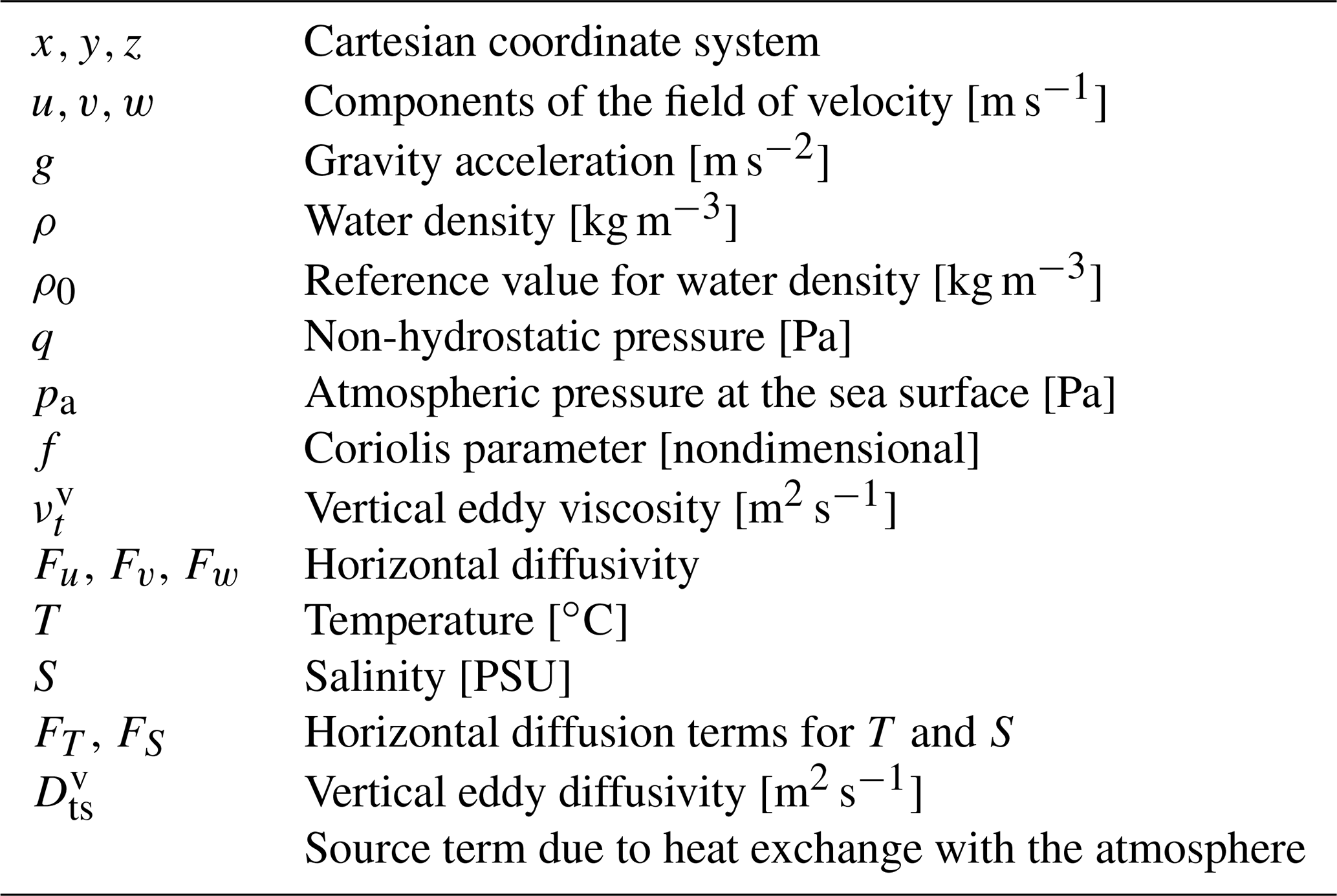
The MIKE 3 Flow Model FM is based on the Navier–Stokes equations for an incompressible fluid under the assumptions of Boussinesq. The governing equations of the model are the equations of momentum (A1) and mass continuity (A2), the equations of heat and salinity transport (A3 and A4, respectively), and the equation of state (A5) based on the UNESCO formula of 1981 (UNESCO, 1981a). Considering a Cartesian coordinate system $(x,y,z)$ we have

$$\begin{array}{}\text{(A1)}& {\displaystyle \frac{\partial u}{\partial x}}+{\displaystyle \frac{\partial v}{\partial y}}+{\displaystyle \frac{\partial w}{\partial z}}=\mathrm{0}\end{array}$$

$$\begin{array}{}\text{(A2a)}& {\displaystyle }\begin{array}{rl}{\displaystyle \frac{\partial u}{\partial t}}+{\displaystyle \frac{\partial u^{\mathrm{2}}}{\partial x}}+{\displaystyle \frac{\partial vu}{\partial y}}+{\displaystyle \frac{\partial wu}{\partial z}}& =fv-{\displaystyle \frac{\mathrm{1}}{{\mathit{\rho }}_{\mathrm{0}}}}{\displaystyle \frac{\partial q}{\partial x}}-g{\displaystyle \frac{\partial \mathit{\eta }}{\partial x}}\\ & -{\displaystyle \frac{\mathrm{1}}{{\mathit{\rho }}_{\mathrm{0}}}}{\displaystyle \frac{\partial p_{\mathrm{a}}}{\partial x}}-{\displaystyle \frac{g}{{\mathit{\rho }}_{\mathrm{0}}}}{\int }_z^{\mathit{\eta }}{\displaystyle \frac{\partial \mathit{\rho }}{\partial x}}\mathrm{d}z\\ & +F_u+{\displaystyle \frac{\partial }{\partial z}}\left({\mathit{\nu }}_t^{\mathrm{v}}{\displaystyle \frac{\partial u}{\partial z}}\right)\end{array}\text{(A2b)}& {\displaystyle }\begin{array}{rl}{\displaystyle \frac{\partial v}{\partial t}}+{\displaystyle \frac{\partial v^{\mathrm{2}}}{\partial y}}+{\displaystyle \frac{\partial uv}{\partial x}}+{\displaystyle \frac{\partial wv}{\partial z}}& =fu-{\displaystyle \frac{\mathrm{1}}{{\mathit{\rho }}_{\mathrm{0}}}}{\displaystyle \frac{\partial q}{\partial y}}-g{\displaystyle \frac{\partial \mathit{\eta }}{\partial y}}\\ & -{\displaystyle \frac{\mathrm{1}}{{\mathit{\rho }}_{\mathrm{0}}}}{\displaystyle \frac{\partial p_{\mathrm{a}}}{\partial y}}-{\displaystyle \frac{g}{{\mathit{\rho }}_{\mathrm{0}}}}{\int }_z^{\mathit{\eta }}{\displaystyle \frac{\partial \mathit{\rho }}{\partial y}}\mathrm{d}z\\ & +F_v+{\displaystyle \frac{\partial }{\partial z}}\left({\mathit{\nu }}_t^{\mathrm{v}}{\displaystyle \frac{\partial v}{\partial z}}\right)\end{array}\text{(A2c)}& {\displaystyle }\begin{array}{rl}{\displaystyle \frac{\partial w}{\partial t}}+{\displaystyle \frac{\partial w^{\mathrm{2}}}{\partial z}}+{\displaystyle \frac{\partial uw}{\partial x}}+{\displaystyle \frac{\partial wv}{\partial y}}& =-{\displaystyle \frac{\mathrm{1}}{{\mathit{\rho }}_{\mathrm{0}}}}{\displaystyle \frac{\partial q}{\partial z}}+F_w\\ & +{\displaystyle \frac{\partial }{\partial z}}\left({\mathit{\nu }}_t^{\mathrm{v}}{\displaystyle \frac{\partial w}{\partial z}}\right)\end{array}\end{array}$$

$$\begin{array}{}\text{(A3)}& {\displaystyle \frac{\partial T}{\partial t}}+{\displaystyle \frac{\partial uT}{\partial x}}+{\displaystyle \frac{\partial vT}{\partial y}}+{\displaystyle \frac{\partial wT}{\partial z}}=F_T+{\displaystyle \frac{\partial }{\partial z}}\left(D_{\mathrm{ts}}^{\mathrm{v}}{\displaystyle \frac{\partial T}{\partial z}}\right)+\text{(A4)}& {\displaystyle \frac{\partial S}{\partial t}}+{\displaystyle \frac{\partial uS}{\partial x}}+{\displaystyle \frac{\partial vS}{\partial y}}+{\displaystyle \frac{\partial wS}{\partial z}}=F_{\mathrm{s}}+{\displaystyle \frac{\partial }{\partial z}}\left(D_{\mathrm{ts}}^{\mathrm{v}}{\displaystyle \frac{\partial S}{\partial z}}\right)\text{(A5)}& {\displaystyle }\mathit{\rho }=\mathit{\rho }(S,T).\end{array}$$

As we used the barotropic density mode, the only hydrodynamic equations used for the present work are Eqs. (A1) and (A2). The symbols used in the governing equations of the model are presented in Table A1.

Table A1 Symbols used in the governing Eq. (A1).

Appendix B: Mud transport model governing equations and parameterizations

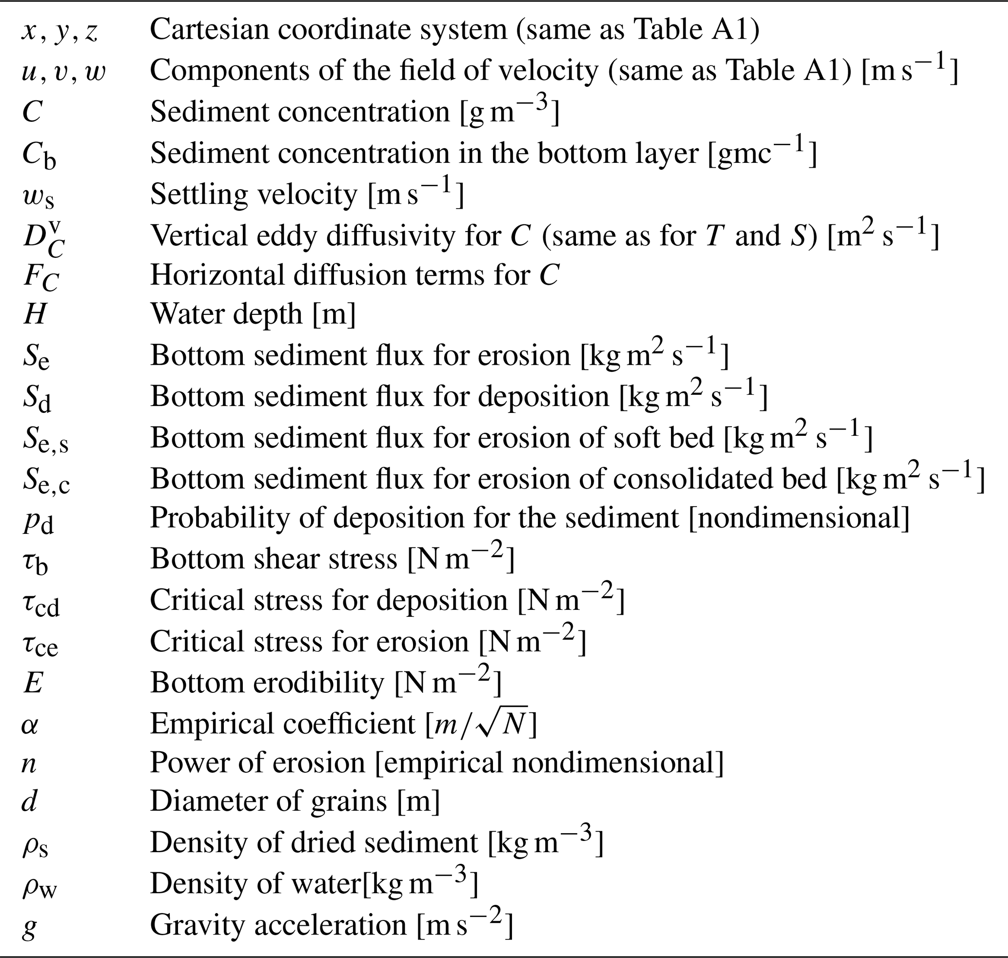
The sediment transport module is based on the advection dispersion equation for a passive tracer in an incompressible fluid. The tracer is the concentration C of the sediment along the water column. The field velocity used for advection is the one calculated through the hydrodynamic set of equations in Appendix A. The symbols used in the following set of equations are summarized in Table B1.

$$\begin{array}{}\text{(B1)}& \begin{array}{rl}{\displaystyle \frac{\partial C}{\partial t}}& +{\displaystyle \frac{\partial }{\partial x}}\left(uC\right)+{\displaystyle \frac{\partial }{\partial y}}\left(vC\right)+{\displaystyle \frac{\partial }{\partial z}}\left[\left(w+w_{\mathrm{s}}\right)C\right]\\ & ={\displaystyle \frac{\partial }{\partial z}}\left(D_C^{\mathrm{v}}{\displaystyle \frac{\partial C}{\partial z}}\right)+F_C\end{array}\end{array}$$

The vertical bottom boundary condition for sediment flux is expressed as

$$\begin{array}{}\text{(B2)}& D_C^{\mathrm{v}}{\left.{\displaystyle \frac{\partial C}{\partial z}}\right|}_{z=-H}-w_{\mathrm{s}}C=S,\end{array}$$

and the sediment flux S at the bottom is calculated using the approach of Krone (1962) for deposition (Eq. B3), using the approach of Partheniades (1965) for erosion of consolidated sediment (Eq. B5), and using the approach of Parchure and Metha (1985) for erosion of soft or unconsolidated sediment (Eq. B6).

$$\begin{array}{}\text{(B3)}& S_{\mathrm{d}}=w_{\mathrm{s}}{C}_{\mathrm{b}}{p}_{\mathrm{d}},\end{array}$$

where

$$\begin{array}{}\text{(B4)}& {\displaystyle }{p}_{\mathrm{d}}=\mathrm{1}-{\displaystyle \frac{{\mathit{\tau }}_{\mathrm{b}}}{{\mathit{\tau }}_{\mathrm{cd}}}}\text{is valid for}{\mathit{\tau }}_{\mathrm{b}}<{\mathit{\tau }}_{\mathrm{cd}}\text{(B5)}& {\displaystyle }{S}_{\mathrm{e},\mathrm{c}}=E{\left({\displaystyle \frac{{\mathit{\tau }}_{\mathrm{b}}}{{\mathit{\tau }}_{\mathrm{ce}}}}-\mathrm{1}\right)}^n\text{is valid for}{\mathit{\tau }}_{\mathrm{b}}\ge {\mathit{\tau }}_{\mathrm{ce}}\text{and hard bed}\text{(B6)}& {\displaystyle }\begin{array}{rl}{S}_{\mathrm{e},\mathrm{s}}=E\exp \left[\mathit{\alpha }{\left({\mathit{\tau }}_{\mathrm{b}}-{\mathit{\tau }}_{\mathrm{ce}}\right)}^{\mathrm{1}/\mathrm{2}}\right]& \text{is valid for}{\mathit{\tau }}_{\mathrm{b}}\ge {\mathit{\tau }}_{\mathrm{ce}}\\ & \text{and soft bed}.\end{array}\end{array}$$

The settling velocity for sediment is calculated through the Stokes' law Eq. (B7).

$$\begin{array}{}\text{(B7)}& w_{\mathrm{s}}={\displaystyle \frac{g{d}^{\mathrm{2}}}{\mathrm{18}}}\left({\displaystyle \frac{{\mathit{\rho }}_{\mathrm{s}}}{{\mathit{\rho }}_{\mathrm{w}}}}-\mathrm{1}\right)\end{array}$$

Table B1 Symbols used in Eq. (B1) to (B7) and the associated parameterizations of the sediment transport model.

Appendix C: Results of total bed change

The following matrices of plots (Fig. C1) present the results in terms of sediment erosion and accumulation for the scenarios for docks T1, T2, T3, T5, and T6 (top to bottom, left part of Fig. C1) and T9, T10, T11, DL, and 1003 (top to bottom, right part of Fig. C1). Undocking and docking phases are represented in the left and right panels, respectively.

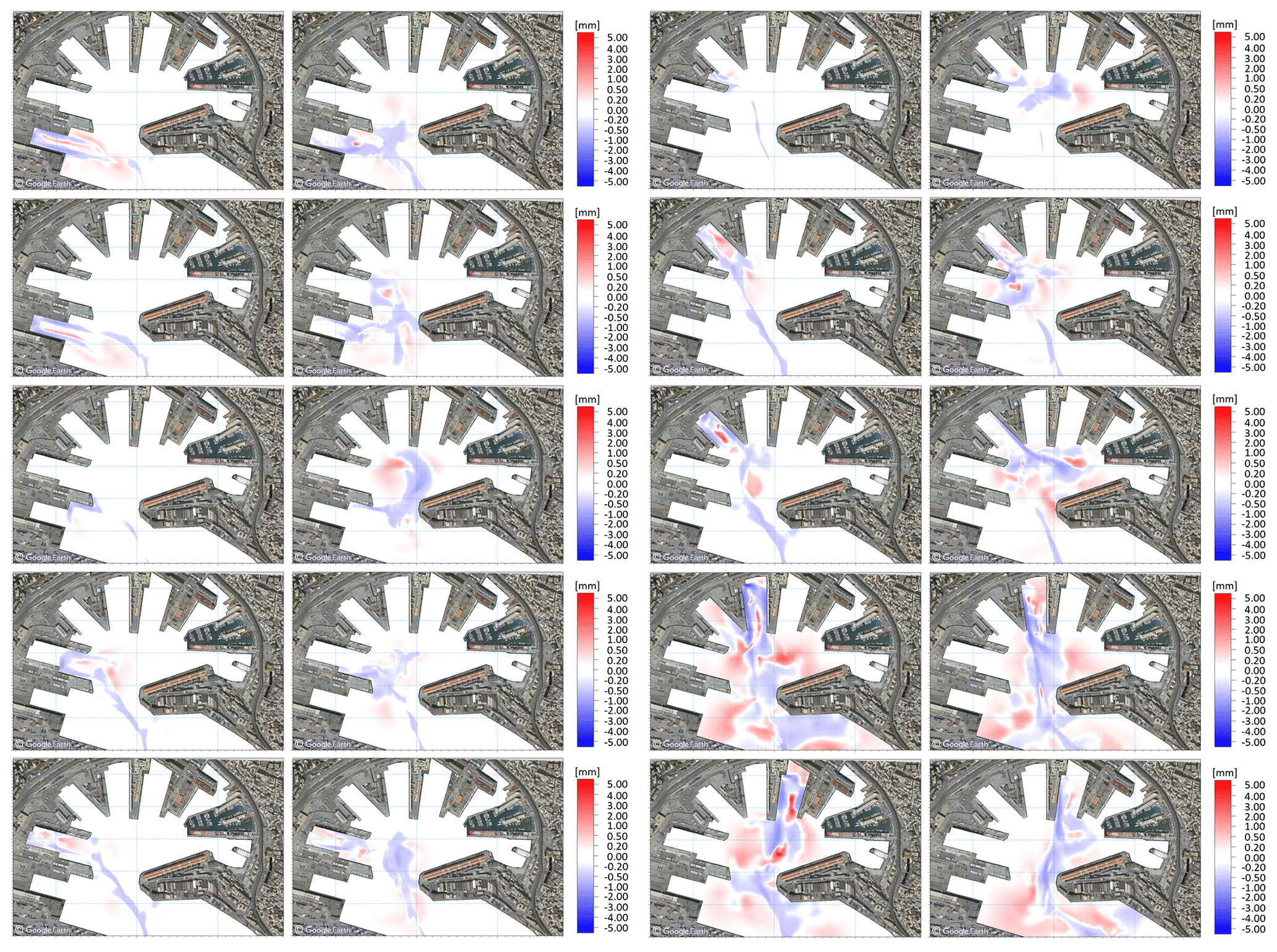
Figure C1 Sediment erosion and accumulation for the scenarios of docks T1, T2, T3, T5, and T6 (left, top to bottom) and for the scenarios of docks T9, T10, T11, DL, and 1003 (right, top to bottom). Land background from © Google Earth.