the Creative Commons Attribution 4.0 License.
the Creative Commons Attribution 4.0 License.
 | 04 Feb 2021
Properties of surface water masses in the Laptev and the East Siberian seas in summer 2018 from in situ and satellite data
Alexandre Supply
Nikita Kusse-Tiuz
Vladimir Ivanov
Mikhail Makhotin
Jean Tournadre
Bertrand Chapron
Jacqueline Boutin
Nicolas Kolodziejczyk
Gilles Reverdin
Variability of surface water masses of the Laptev and the East Siberian seas in August–September 2018 is studied using in situ and satellite data. In situ data were collected during the ARKTIKA-2018 expedition and then complemented with satellite-derived sea surface temperature (SST), salinity (SSS), sea surface height, wind speed, and sea ice concentration. The estimation of SSS fields is challenging in high-latitude regions, and the precision of soil moisture and ocean salinity (SMOS) SSS retrieval is improved by applying a threshold on SSS weekly error. For the first time in this region, the validity of DMI (Danish Meteorological Institute) SST and SMOS SSS products is thoroughly studied using ARKTIKA-2018 expedition continuous thermosalinograph measurements and conductivity–temperature–depth (CTD) casts. They are found to be adequate to describe large surface gradients in this region. Surface gradients and mixing of the river and the sea water in the ice-free and ice-covered areas are described with a special attention to the marginal ice zone at a synoptic scale. We suggest that the freshwater is pushed northward, close to the marginal ice zone (MIZ) and under the sea ice, which is confirmed by the oxygen isotope analysis. The SST-SSS diagram based on satellite estimates shows the possibility of investigating the surface water mass transformation at a synoptic scale and reveals the presence of river water on the shelf of the East Siberian Sea. The Ekman transport is calculated to better understand the pathway of surface water displacement on the shelf and beyond.
- Article
(21105 KB) - Full-text XML
- BibTeX
- EndNote


The eastern part of the Eurasian Arctic remains one of the less studied areas of the Arctic Ocean. Carmack et al. (2016) described this region as an “interior shelf” (the Kara sea, the Laptev sea, the East Siberian sea, and the Beaufort sea), where 80 % of the Arctic basin river discharge is released. Armitage et al. (2016) estimated the annual river water input as 2000 m3. The Arctic Ocean stores 11 % of global river discharge, and thus its role in a planetary water budget deserves a special attention. The surface stratification and the freshwater content are regarded as key parameters that have to be followed to better understand the changing state of a “New Arctic” climate (Carmack et al., 2016). Johnson and Polyakov (2001) discussed the salinification of the Laptev sea from 1989 up to 1997, explaining it as being due to the eastward freshwater displacement and an excessive brine release in the sea ice leads. A more recent study reports that a 20 % increase in the Eurasian river runoff has been observed over the last 40 years (Charette et al., 2020). Overall, a freshening of the American basin of the Arctic Ocean was reported in 2000–2010 (Carmack et al., 2016), and at the same time a decrease in a freshwater content of about 180 km3 between 2003 and 2014 was calculated from altimetry measurements by Armitage et al. (2016) over the Siberian shelf. The importance of shelf seas for the freshwater content storage and distribution was outlined in several recent studies (Haine et al., 2015; Armitage et al., 2016; Carmack et al., 2016). The importance of the exchange between the shelf seas and the deep basin is large: 500 km3 for the Laptev and the East Siberian seas, with anticyclonic atmospheric vorticity “on quasi-decadal timescales”, calculated from 1920–2005 hydrographic measurements by Dmitrenko et al. (2008). Previously, the Arctic shelf was considered a “short-term buffer” (3.5±2 years) storing the river water before it enters into the deeper central part and is transported by the Transpolar Drift (9–20 years) to the North Atlantic through the Fram Strait (Schlosser et al., 1994). A recent study of Charette et al. (2020) shows that the “intensification of the hydrologic cycle” will speed up the transport of the freshwater, carbon, nutrients and trace elements from the shelf to the central Arctic and further: the trace elements and isotopes move from the shelf edge to the Transpolar Drift stream over 3–18 months, and the Transpolar Drift takes 1–3 years.
Processes taking place on the eastern Eurasian Arctic shelf are important for the redistribution of the freshwater arriving there and its further path, while the amount of fresh water is expected to increase (Carmack et al., 2016; Charette et al., 2020). A complex topography, several sources of fresh and saline water masses, and unstable atmospheric conditions and ocean processes, such as mesoscale activity and tidal currents, can alter the direction of the freshwater distribution. Close to the coast the riverine water from several sources is expected to propagate eastward as a “narrow (1–20 km) and shallow (10–20 m) feature” (Carmack et al., 2016; Lentz, 2004), but its transformation and mixing with a saline seawater and sea ice melting and freezing are less studied. The Laptev and the East Siberian shelf areas were described as a substantial region of sea ice production for the central Arctic (Ricker et al., 2017), and to better estimate the impact of the incoming freshwater on the sea ice formation, the freshwater pathways in the Arctic should be better understood. Despite several studies on the freshwater in the eastern Arctic (e.g., Semiletov et al., 2005; Dmitrenko et al., 2012; Osadchiev et al., 2017; Bauch and Cherniavskaia, 2018), to the best of our knowledge, no study has yet shown the evolution of the water masses on a synoptic scale in the Laptev Sea, except a very recent one by Osadchiev et al. (2020), which has been done in parallel with this study but on the basis of other in situ data. In this paper, we look at the information accessible with satellite salinity. The salinity provides precious information about the fate of the freshwater river input. While this information is restricted to the top sea surface, the regular and synoptic monitoring of sea surface salinity from space allows us to document its spatiotemporal variability in great detail that would not be accessible with any other means, providing a new tool for analyzing some of the processes at play.
The Laptev Sea is shallow in its southern and central parts (less than 100 m) with a very deep opening in the north (3000 m) (Fig. 1). Several water masses are mixed in the Laptev Sea. The Lena, Khatanga, Anabar, Olenyok, and Yana rivers discharge fresh water in the shallowest part of the Laptev Sea in the south. The Kara Sea's waters enter via the Vilkitskiy and the Shokalskiy straits, the Atlantic Water (AW) propagates along the continental slope to the north of the Severnaya Zemlya Archipelago and further eastward, and the Arctic Water is found in the sea's northern part (Rudels et al., 2004; Janout et al., 2017; Pnyushkov et al., 2015). The direction of the surface freshwater circulation is supposed to correspond to a general displacement of the intermediate Atlantic Water: mainly eastward following the coastline (Carmack et al., 2016). This eastward transport brings the water masses of the Laptev Sea over the shelf of the East Siberian Sea where they meet Pacific-origin waters (Lenn et al., 2009; Semiletov et al., 2005).
In the Arctic region, a strong seasonality of air–sea heat flux and sea ice melting and freezing modify the temperature and the salinity in the upper layer and therefore result in a vertical structure of the water column with fronts at the surface and “modified layers” in the interior (Rudels et al., 2004; Pfirman et al., 1994; Timmermans et al., 2012). The most common concept of the upper ocean layer is a “mixed layer” concept: between an ocean surface being in contact with the atmosphere and a certain depth, the temperature and the salinity are homogeneous. A mixed layer extends down to a specified vertical gradient in density and/or temperature (de Boyer Montégut et al., 2004; Timokhov and Chernyavskaya, 2009) or a maximum of Brunt–Väisälä frequency (Vivier et al., 2016). In the Arctic, the reported mixed layer depth (MLD) varies between 5 and 50 m depending on region, time, and whether it is measured in open water or under ice (10 m in the Laptev and the East Siberian seas and 5 m in the central Arctic Ocean and northern Barents Sea in summer, Timokhov and Chernyavskaya, 2009; 10–15 m in the Beaufort Sea close to the marginal ice zone (MIZ) in summer, Castro et al., 2017; 20 m in the Barents Sea in late summer, Pfirman et al., 1994; 40–50 m under the ice close to the North Pole in winter, Vivier et al., 2016).
At the same time, Timmermans et al. (2012) proposed using the term “surface layer” instead of “mixed layer” for the Arctic Ocean because a water layer lying between the sea surface and the Arctic main halocline can be weakly stratified even though the halocline hampers an active exchange of matter and energy. The main halocline is situated at 50–100 m depth in the eastern Arctic (Dmitrenko et al., 2012) and at 100–200 m depth in the western Arctic Ocean (Timmermans et al., 2012). Using concept of the “surface layer”, the processes in that layer can be discussed separately from the ones in the deeper layer. The freshwater is expected to be delivered to the central (European) Arctic from the Siberian shelf, roughly along the Lomonosov Ridge and to the western Arctic, partly along the continental slope (Charette et al., 2020).
The position of the pycnocline in the Arctic is mostly defined by salinity. One of the first studies of Aagaard and Carmack (1989) devoted to the freshwater content was using 34.80 as a reference salinity value separating the “fresh” and the “saline” water; 34.80 was considered a mean Arctic Ocean salinity at that time. This value is also used in more recent overviews (e.g., Haine et al., 2015; Carmack et al., 2016) and helps to define “Atlantic Water” as saltier than this value. Rabe et al. (2011) used a 34 isohaline depth to estimate a liquid freshwater content in the Arctic Ocean. Carmack et al. (2016) considered a depth of a “near-freezing freshwater mixed layer” in the Eurasian Arctic Ocean to be 5–10 m. Cherniavskaia et al. (2018) reported an overall salinity in the upper 5–50 m layer within the range from 30.8 to 33 based on in situ data in the Laptev Sea during 1950–1993 and 2007–2012. Between the very surface layer and the Atlantic Water, Dmitrenko et al. (2012) found the modified “Lower Halocline” Water with typical characteristics of salinity between 33 and 34.2 and a negative temperature (below −1.5 ∘C); in 2002–2009 this layer was situated at 50–110 m depth. The study of Polyakov et al. (2008) on Arctic Ocean freshening defined the upper ocean layer to be between 0 m and a depth of a density layer σθ=27.35 kg m−3. This isopycnal is often located at 140–150 m depth, “slightly above the Atlantic Water upper boundary defined by the 0 ∘C isotherm”.
The stable vertical stratification is modified by mixing. Mixing can be induced by winds generating surface-intensified Ekman currents, mesoscale dynamics (eddies), and a shear in tidal and other currents (Carmack et al., 2016; Lenn et al., 2009; Rippeth et al., 2015). Tidal currents and internal waves amplified over the shelf edge are associated with the mixing in the interior of the water column, below or in the main Arctic pycnocline (Rippeth et al., 2015; Lenn et al., 2009, 2011).
Temperature and salinity fronts separate well-mixed water masses. Dmitrenko et al. (2005) and Bauch and Cherniavskaia (2018) showed that interannual changes of river discharge and wind patterns define the position of oceanographic fronts in the central part of the Laptev Sea. Based on model results, Johnson and Polyakov (2001) showed that in 1989–1997 the freshwater was driven eastward under the influence of winds associated with a “strong cyclonic vorticity over the Arctic”. The same study demonstrated that the associated salinification of the central Arctic Ocean weakened the vertical stratification of the water column. The anticyclonic regime is considered to increase the salinity of the shelf seas (Armitage et al., 2016). Armitage et al. (2017) discuss the importance of sea ice, as it creates a surface drag and establish the Ekman transport of the freshwater in the surface layer, which in turn impacts the dynamical ocean topography and geostrophic currents in the Arctic Ocean. Armitage et al. (2018) further mention that alongshore winds correlated with AO (Arctic Oscillation) index create the onshore Ekman transport, changing water properties over the shelf.
In the seasonal cycle, the summer season is of a particular interest for all Arctic studies. The sea ice melting usually starts in June and ends in August–September, while the sea ice formation can start already in September, and by November the Laptev Sea is already completely sea-ice covered. The East Siberian Sea is usually covered by the sea ice most of the year, and is exposed to the air-sea interaction for a shorter period of time (in August–September) over a smaller ice-free surface than the Laptev Sea. August and September are two summer months that are very important for the heat exchange between the open ocean and the atmosphere over the Laptev Sea. In a recent study, Ivanov et al. (2019) reported that during this time period when the sea ice is melting and the ocean is opening, the net radiative balance at the sea surface changes from 100 W m−2 to zero values, following the seasonal cycle of shortwave radiation (meaning the flux from the atmosphere to the ocean). The sea level anomalies over the eastern Arctic shallow seas are positive and largest in summer (up to 10 cm at 75∘ N, down to 3 cm at 80∘ N, as reported by Andersen and Johannessen, 2017). The seasonal peak of the maximum freshwater content over the shelf is found in summertime when the river discharge is the highest, while the freshwater content minimum (following export of this accumulated freshwater) occurs in March, when the freshwater captured by sea ice is advected away from the shelf (Armitage et al., 2016; Ricker et al., 2017).
The Laptev Sea is not at all sampled by Argo products, so the recent ARKTIKA-2018 expedition measurements combined with novel satellite sea surface salinity and other satellite-derived parameters provide an unprecedented documentation of the temporal evolution of the surface water properties in the Laptev and East Siberian seas during summer 2018. In this study, we propose following the upper ocean water displacement and discuss what causes it on a daily basis.
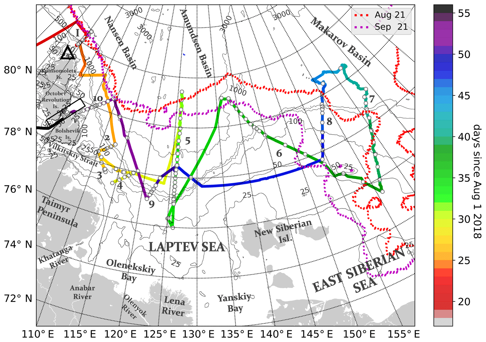
Figure 1Legs and stations of the ARKTIKA-2018 expedition overlaid on the bathymetry from ETOPO1 “1 arcmin Global Relief Model” (Amante and Eakins, 2009). CTD stations are shown with white dots. The color indicates the number of days since 1 August 2018. The sea ice edge position is indicated with a dashed red line for the beginning (21 August) and with a dashed purple line for the end of the expedition (21 September). The ice edge is based on the sea ice mask provided in the DMI SST product. Numbers indicate positions of 10 oceanographic transects discussed below. The black triangle in the north of the Komsomolets Island shows the Arkticheskiy Cape. The Severnaya Zemlya Archipelago consists mainly of the Komsomolets, the October Revolution, and the Bolshevik Islands (with smaller islands not shown here). The black box indicates the Shokalskiy Strait between the October Revolution and the Bolshevik Islands. The Yana river estuary (outside the map area) is south of Yanskiy Bay
To analyze the upper-ocean processes, we will focus on the surface layer with satellite data and on the upper 250 m layer with the CTD (conductivity, temperature, depth) casts, providing the isohaline and isopycnal positions. Such an approach to the upper layer is required to estimate the upper limit of the Atlantic Water, which is one of the key contributors to the water mass transformation. The surface water evolution of the Laptev and the East Siberian seas is described and discussed with respect to changes in wind speed and direction during the ARKTIKA-2018 expedition.
2.1 In situ measurements during the ARKTIKA-2018 expedition
Oceanographic measurements during the ARKTIKA-2018 expedition on board RV Akademik Tryoshnikov started on 21 August 2018 and ended on 24 September 2018 (Fig. 1). Oceanographic transects were organized to take into account the requirements of different scientific expeditions on board, NABOS (Nansen and Amundsen Basin Observational System) and CATS (Changing Arctic Transpolar System) to observe shallow and continental slope processes. NABOS transects were mostly cross-shelf (1, 5, 6–8, 10), and CATS transects were shallower (2–4, 9). Transects 3 and 10 were made in the straits between the Kara and the Laptev seas: transect 3 in the Vilkitskiy Strait southward to the Bolshevik Island, with depths from 70–200 m opening into the deep central part of the Laptev Sea (more than 1000 m), and transect 10 in the narrow and rather shallow (250 m) Shokalskiy Strait between the Bolshevik and the October Revolution Islands. Some measurements were carried out in the MIZ and ice-covered area (see the sea ice edge positions at the beginning and the end of the cruise in Fig. 1). In this study we define MIZ as an area with 0 %–30 % sea ice concentration close to the ice edge. Standard oceanographic stations (145 in total) were conducted with a SeaBird SBE911plus CTD instrument equipped with additional sensors. For this study, we use mainly the CTD measurements of potential temperature and practical salinity but also the results of oxygen isotope analysis from the first (surface) bottle samples (Alkire and Rember, 2019). All CTD data were processed and quality checked. The cruise data can be found at https://arcticdata.io/catalog/data, last access: 24 January 2021 (Polyakov and Rember, 2019) and Ivanov (2019).
The ship was equipped with an underway measurement system Aqualine Ferrybox, widely known as a thermosalinograph (TSG). The instrument had a temperature and a conductivity (MiniPack CTG, CTD-F) sensors and a CTG UniLux fluorometer installed; thus, continuous temperature, salinity, and chlorophyll-a estimations were obtained along the ship's trajectory. The inflow is situated at 6.5 m below the surface (the inflow hole is on the ship's hull). All data were processed and filtered for random noise and poor quality measurements and then compared and calibrated with CTD measurements. When calculating a linear regression between CTD measurements at 6.5 m depth and TSG measurements, we obtain a good correlation for both temperature and salinity (correlation coefficient equal to 0.979 and 0.966, respectively, not shown). The standard error is 0.023∘ for temperature and 0.025 for salinity, and the standard deviation (SD) for the difference of measurements (CTD minus TSG) was SDtemp=0.413 ∘C and SDsal=0.423. To adjust the continuous TSG measurements to the more precise CTD measurements, we applied the obtained linear regression equation to TSG data. We only use these adjusted temperature and salinity data.
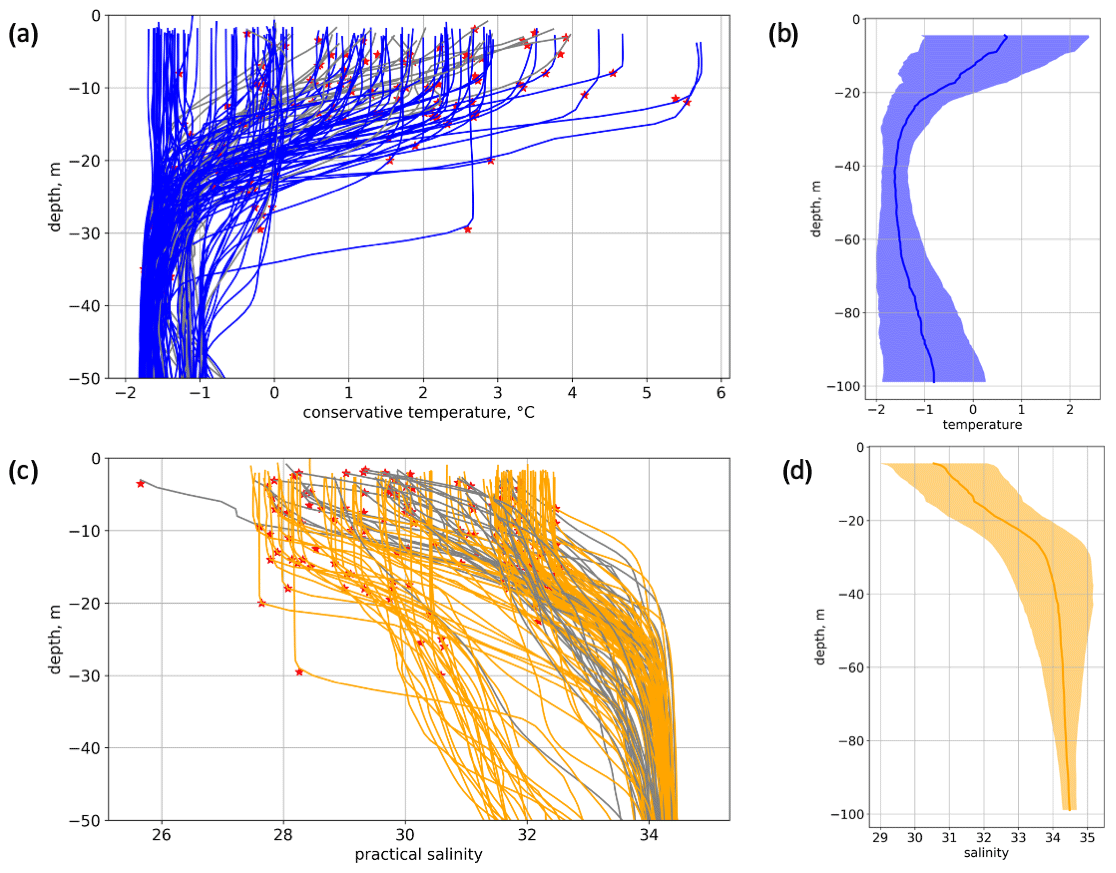
Figure 2Vertical profiles of conservative temperature (a, b) and practical salinity (c, d) from CTD measurements in the upper ocean layer. Panels (a) and (c) show all vertical profiles in the upper 50 m, calculated using de Boyer Montégut et al. (2004) method (see details in the text): red stars indicate the mixed layer depth, colored profiles show the cases when the MLD is below 7 m depth, and gray profiles indicate when the MLD is above 7 m depth. Panels (b) and (d) show the median vertical profiles in the 5–100 m layer of temperature and salinity, respectively, where the shaded area shows the associated SD.
The vertical profiles of the conservative temperature and practical salinity in the upper layer are presented in Fig. 2. To investigate if the TSG measurements can be used to study the surface layer in a highly stratified Laptev sea, we calculated a summer mixed layer depth following the de Boyer Montégut et al. (2004) method based on density and temperature gradient thresholds (Fig. 2a, c). The MLD is found at a depth of the first maximum temperature gradient below a depth of defined (by given threshold) density gradient (see de Boyer Montégut et al. (2004) for details). Using the same approach, we computed MLD with density and salinity vertical profiles. The threshold chosen for practical density gradient was 0.3 kg m−3 m−1 and 0.2 units per 1 m for conservative temperature and practical salinity gradients. Regarding the MLD calculated from salinity (MLDsal), most of the measured vertical profiles (75.17 %) had the MLDsal below 7 m depth with the median of MLDsal 11.99 m. As for the temperature (MLDtemp), 81.37 % of the measured profiles had the MLD below 7 m depth with a median of MLDtemp=13.50 m. Thus, in most cases the upper 12 m of the surface layer was homogeneous, and the CTD and TSG measurements can be used for the validation of satellite data. The median vertical profiles of temperature and salinity in the upper 5–100 m are presented in addition to the associated SD in Fig. 2b, d). We observe rather cold (0.5 ∘C) and fresh (30.5) water at 5 m, followed by a smooth thermocline and halocline down to 30 m depth (with a temperature of −1.3 ∘C and salinity of 33.8). Below 30 m the temperature rises slightly to −1 ∘C and salinity stays close to 34.5. The SD of conservative temperature is the largest at the surface (1.55 ∘C) and smallest at 40 m depth (0.27 ∘C). The SD of salinity is also the largest at the surface (1.50) but diminishes with depth to 0.20 at 100 m. Nevertheless, it is clear that at the end of a summer season in this region with very different water origins, these median profiles are not representative for all water masses. Additionally, we did an important number of CTD casts in very shallow areas with depths between 30 and 50 m, and thus the calculated averaged (median) vertical profile is composed of “shallow” and “deep” vertical profiles. We do not include the very surface measurements above 5 m because we only had 45 CTD measurements at 2 m depth among the 146 possible and taking them into account would bias the median profiles as well.
2.1.1 River discharge
To illustrate the amount and temporal variability of the river discharge in 2018, we used daily measurements of the Lena River discharge from the Arctic Great Rivers Observatory (GRO) dataset (https://arcticgreatrivers.org/data/, last access: 24 January 2021). In Fig. 3 we present a time series of the Lena River discharge from May to November 2018. The river stayed under the ice with a very small discharge up to the end of May. The main peak of the Lena River discharge occurred in the beginning of the Arctic summer in June and corresponds to the snow and ice melting over the river basin in Siberia. Over 2 weeks, the discharge changed from 2500 to 120 000 m3 s−1. The second, smaller peak of the river discharge occurred at the beginning of August (60 000 m3 s−1), which might be associated with summer precipitation. During August 2018 the river discharge decreased from 60 000 to 40 000 m3 s−1, and in September it varied very little, staying close to 40 000 m3 s−1. A significant diminution of the river discharge started in the beginning of October and continued up to the beginning of November. After the beginning of November the river discharge was very weak and close to its minimum values (4500 m3 s−1).
The described seasonal dynamics are typical for the Lena River and consistent with existing results, e.g., those demonstrated in Janout et al. (2015). They can be complemented by the results of the Papa et al. (2008) study of the large Siberian rivers using satellite data. Papa et al. (2008) showed that the maximum of precipitation over the basins of the Lena, the Ob, and the Yenisey rivers occurs in July, and the mean monthly air temperature is at its maximum at that time.
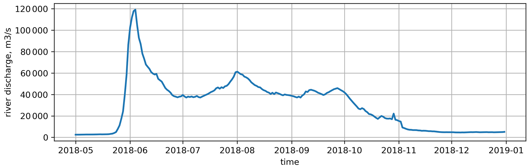
Figure 3The Lena River discharge in 2018. Data taken from the Arctic GRO dataset (https://arcticgreatrivers.org/data/, last access: 24 January 2021).
2.2 Satellite data
Satellite data provide information on the surface distribution of geophysical characteristics over the whole study area together with their temporal evolution.
All products listed below are considered from 1 August to 25 September 2018 (the last day of ARKTIKA-2018 expedition). For consistency, when not specifically indicated, all products are linearly interpolated on a regular grid within the box 74–85∘ N, 90–170∘ E, with a 0.01∘ step in latitude and 0.05∘ in longitude. The spatial resolution of the selected grid roughly corresponds to 1 km.
2.2.1 Sea surface temperature
The sea surface temperature (SST)-retrieving instruments with the highest resolution, such as AVHRR (Advanced Very High Resolution Radiometer), MODIS (Moderate Resolution Imaging Spectroradiometer), and VIIRS (Visible Infrared Imaging Radiometer Suite), work in near-infrared (NIR) and infrared (IR) bands and strongly depend on atmospheric conditions (providing measurements only for clear sky without clouds). For lower-resolution microwave instruments, such as AMSR2 (Advanced Microwave Scanning Radiometer 2), the clouds are transparent, but the SST retrievals may still be hampered by high wind speed and precipitation events. As satellite measurements in IR and NIR ranges are sparse because of the frequent cloudiness over the Arctic Ocean, we used a blended product. In this paper we use the Danish Meteorological Institute Arctic Sea and Ice Surface Temperature product (hereafter referred to as “DMI SST”). DMI SST is a Level 41 daily product provided by the Copernicus Marine service. Daily surface temperatures over the sea and ice are derived on a 5 km spatial grid from several instruments: AVHRR, VIIRS for SST, and AMSR2 for sea ice concentration using optimal interpolation (Høyer et al., 2014).
Besides the full coverage over the studied area, the advantage of the blended DMI SST product is that it takes into account the ice temperature, and thus the marginal ice zone is better represented and not masked out. The total number of SST measurements ingested over the studied area from 1 August to 25 September 2018 varies from 1000 to 2500 measurements per pixel.

Figure 4Sea surface temperature validation shown with an example of a DMI SST L4 image for 13 September (a) and the same image shown with the error estimates (b), a comparison of colocated SST and in situ data (CTD and TSG) in the upper 6.5 m (c), and the distribution of uncertainty provided by DMI and absolute difference derived from comparison with in situ data (d).
2.2.2 Validation of DMI SST
The first step of the DMI SST validation was its value-by-value comparison with a colocated in situ dataset (nearest-neighbor DMI SST pixel). For this analysis, we colocated DMI SST with the in situ potential temperature measurements in the upper 6.5 m layer: all available CTD measurements averaged every half a meter above 6.5 m depth and all TSG measurements at 6.5 m depth averaged every 30 min. The median depth of the colocated CTD measurements is 5.25 m. As for the TSG, the ship was moving with a median speed of 8 kn during the cruise, and thus an average of 30 min TSG measurements is an average over approximately 7.5 km. Thus, a 30 min TSG average is comparable with one DMI SST pixel (10 km). There were 1707 colocated points in the analysis.
Although satellite SST estimates may differ from the in situ temperature measurements in the upper 6.5 m, we expect an overall consistency between the datasets. Studies carried out by Castro et al. (2017) devoted to the validation of MODIS SST in the MIZ and by Vivier et al. (2016), which described in situ measurements in the iced-covered area, reported that the first 7–10 m layer below the surface was mostly homogeneous. As is shown in Fig. 2, most of our measurements (more than 75 %) were homogeneous in the upper 12 m (and were done in the ice-free areas). Nevertheless, a diurnal warming and local vertical mixing can affect the vertical temperature distribution in the very surface layer. The SST diurnal amplitude can reach more than 3 K in the Arctic Ocean (Eastwood et al., 2011). To create DMI SST L4 product, only the observations between 21:00 and 07:00 local time are used (Høyer et al., 2014), thus local diurnal variations of SST are supposed to be filtered out. Diurnal variation of temperature might be present in real in situ measurements during strong diurnal warming events, but no particular observations allowing the investigation of this question were done during the cruise.
To illustrate the consistency of SST and in situ temperature datasets, 13 September 2018 was considered, as it was one of the rare days in summer 2018 when the central part of the Laptev Sea was cloud-free, which is especially important for DMI SST.
The DMI SST product for 13 September, presented in Fig. 4a, shows a rather complex pattern with a pronounced gradient associated with warm river water in the central part of the Laptev Sea. The uncertainty in SST estimates provided by DMI is shown in Fig. 4b, d. The percentage of occurrence is computed for 0.5 ∘C temperatures classes starting at 0 ∘C (Fig. 4d). The highest uncertainty (up to 2.5 ∘C) was observed over some open-sea areas that were partially cloudy but was mostly associated with the sea ice due to its heterogeneity (Fig. 4b). Over most of the southern and the central part of the ice-free Laptev and the East Siberian seas, the uncertainty is below 0.5 ∘C, and over the eastern part it is below 1 ∘C.
Comparison of the DMI SST and in situ surface-layer temperature (Fig. 4, c) shows a good agreement that is almost independent of area and time during the ARKTIKA-2018 expedition. The bias (difference between mean DMI and mean in situ surface temperature data) is 0.19 ∘C. This excess average DMI SST seems to be possible, based on CTD measurements, indicating that the 0–3 m water layer is on average 0.3 ∘C warmer than the 3–6.5 m layer (not shown). The largest deviations are observed when the ship is in the MIZ or a more compact sea ice, so they might be associated with either imperfect sea ice flagging of some stages of sea ice in the DMI SST product or a noise introduced after re-interpolation of data on a regular grid. This noise, together with the different sampling of in situ potential temperature measurements and the DMI SST product, lead to a distribution of the absolute differences between in situ and DMI SST that is slightly wider than the one of uncertainties provided in the DMI SST product (Fig. 4d). Nevertheless, this comparison should be taken only as indicative of a reasonable order of magnitude of the uncertainties given the limited number of in situ measurements for each uncertainty range. After removing the bias, the correlation coefficient is 0.89 and the rms difference is 0.77 ∘C. Overall, DMI SST agrees rather well with in situ data, and it captures a small-scale spatial variability of the SST in the ice-free areas (Fig. 4a) well above SST uncertainties, and thus we use this product for the following analysis of SST time series.
2.2.3 Sea surface salinity
Soil Moisture and Ocean Salinity (SMOS) is the first satellite mission carrying an L-band (1.41 GHz) interferometric microwave radiometer, from which measurements are used to retrieve the sea surface salinity (SSS) in the top centimeter of the water. With the recent processing, the standard deviation of the differences between 18 d SMOS SSS and 100 km averaged TSG surface salinity measurements is 0.20 in the open ocean between 45∘ N and 45∘ S (Boutin et al., 2018). However, the precision degrades in cold water as the sensitivity of L-band radiometer signal to SSS decreases when SST decreases, even though this effect on temporally averaged maps is partly compensated for by the increased number of satellite measurements at high latitude (Supply et al., 2020). The possibility of using SSS estimates in cold regions derived from L-Band radiometry has been recently demonstrated by several working groups (Tang et al., 2018; Grodsky et al., 2018; Olmedo et al., 2018). However, existing L32 SSS products, e.g., SMAP CAP/JPL (Soil Moisture Active Passive satellite, a product created using the Combined Active Passive algorithm by Jet Propulsion Laboratory) SSS, or SMOS BEC (Barcelona Expert Center) SSS, are spatially averaged from 60 km to more than 100 km.
SMAP REMSS (Remote Sensing Systems) SSS L3 v3 provides a 40 km resolution version but does not provide a sufficient coverage in the Laptev Sea. The methodology developed in this study to retrieve SMOS SSS aims to maintain SMOS original spatial resolution and retrieve SSS as close as possible to the ice edge.
A new product, hereafter SMOS SSS “A” (“A” for the Arctic Ocean) L3, investigated in this study was computed using SMOS L23 SSS from the ESA (European Space Agency) last processing (v662, Arias and Laboratories, 2017), (Fig. 5a). SMOS L2 SSS are available on the ESA SMOS Online Dissemination website. SMOS SSS are representative of SSS integrated over about 50×50 km2 given the footprint of SMOS radiometric measurements involved in the SSS retrievals. The SMOS ESA L2 SSS products are oversampled over an Icosahedral Snyder Equal Area (ISEA) grid at 15 km resolution. The oversampling on a 15 km grid is possible owing to the image reconstruction of the SMOS interferometric data, but in this processing we do not make any spatial average for SSS fields.
SMOS “A” SSS was obtained as described below. The 7 d running means were computed for each day and each pixel of the ISEA grid, using a temporal Gaussian weighting function with a standard deviation of 3 d. The full width of SMOS ascending and descending orbits swaths was considered in order to take advantage of better temporal and spatial sampling over the Arctic Ocean and to decrease the uncertainty with temporal averaging. In order to eliminate the SSS at very low and high wind speeds because of higher uncertainties, SMOS ESA L2 SSS was considered only if the associated ECMWF (European Centre for Medium-Range Weather Forecasts) wind speed was between 3 and 12 m s−1. SMOS ESA L2 SSS measurements were also weighted relative to the uncertainty of the SSS measurement (as in Yin et al., 2013, Eq. A7). This uncertainty was derived from information provided with the SMOS L2 products, the SSS “theoretical error”, derived from the uncertainty of all the parameters used for retrieving SMOS SSS, multiplied by the normalized χ2 cost function of the SSS retrieval. Dinnat et al. (2019) showed that the Klein and Swift (1977) dielectric constant model was inaccurate at low SST. In order to mitigate this effect, a SST-dependent correction derived from Fig. 16 of Dinnat et al. (2019) (blue-circle line) was applied: SSS.
Finally, a criterion for a SMOS-retrieved pseudo-dielectric constant (ACARD parameter, defined in Waldteufel et al., 2004), was applied to discard SMOS measurements affected by sea ice (discarded when ACARD <45). The uncertainty of SMOS SSS “A” was derived from the propagation of the uncertainty on individual SMOS ESA L2 SSS pixel during 7 d. The uncertainty strongly increases in the vicinity of sea ice (Fig. 5b). For this reason, in the following study, above 75∘ N, all pixels with an SSS weekly uncertainty larger than 0.8 were not considered. South of 75∘ N, a higher threshold was used (1.5) allowing us to maintain some measurements closer to fresh river water from the Lena and the Khatanga rivers near the coast. In this area, the χ2 may increase due to the strong heterogeneity of SSS within SMOS multi-angular brightness temperatures footprints, and the number of measurements is low due to the presence of the coast and islands even without sea ice. The theoretical uncertainty of SMOS SSS “A” field is below 0.5 in the center of the Laptev Sea and up to 2 and higher close to the coastline and MIZ.
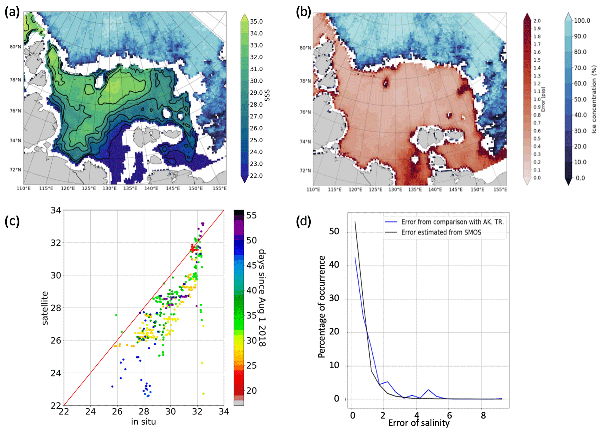
Figure 5Sea surface salinity validation shown with an example of SMOS SSS “A” for 13 September 2018 (a) and associated uncertainties (b), a scatterplot of colocated SSS and in situ data in the upper 6.5 m (c), and statistical distribution of provided SMOS L2 uncertainties and measured absolute difference from comparison with in situ data (d). Sea ice concentration from AMSR2 is indicated with blue shading on the upper panels
2.2.4 Validation of SMOS “A” SSS
In this section, we compared the SMOS SSS “A” relative to in situ measurements. Figure 5 presents the SMOS SSS “A” on 13 September 2018, the same day as the DMI SST in Fig. 4. We colocated SMOS SSS “A” and in situ measurements of salinity in the upper 6.5 m layer in the following manner: the averaging of the TSG salinity was done over a 1 h period (equal to ∼15 km distance, contrary to DMI SST validation) in order to be closer to SMOS SSS “A” spatial resolution. We used 985 colocated points.
Comparison between the in situ practical salinity and SMOS SSS “A” shows a very good agreement that has not yet been demonstrated before by any other salinity product in the Laptev Sea. The mean difference is 2.06, SMOS SSS being lower than in situ surface salinity. This underestimate could be related to the presence of land in the very wide SMOS field of view as observed at lower latitudes by Kolodziejczyk et al. (2016), and this difference appears to be, at first order, systematic (Fig. 5c). In what follows, we subtract this mean difference from the entire SMOS SSS dataset. The correlation coefficient is then 0.86, with a rms difference equal to 0.86. The standard deviation of SMOS SSS with respect to in situ SSS does not vary with the depth of the in situ salinity measurements above 6.5 m, either because in situ salinity was homogeneous vertically or because comparisons were too noisy to detect these small variations (not shown). Although SMOS SSS “A” shows a good agreement most of the time, some larger uncertainties occur close to the sea ice margin or when pixels are contaminated by small ice pattern not detected by AMSR2 sea ice concentration algorithm (as at 80∘ N, 125∘ E in Fig. 5a).
Comparison between SMOS uncertainties and error based on comparison with in situ salinity measurements is presented in Fig. 5d. The percentage of occurrence is computed in salinity classes with a size of 0.5 that starts at 0. It shows a rather good agreement between the distribution of SMOS SSS “A” uncertainties estimated from the retrieval process and the distribution of error obtained from comparison with in situ salinity measurements. The uncertainties are in 85 % of cases less than 1.2, which is relatively small compared to spatial gradients shown on Fig. 5a. These results allow us to use the SMOS SSS “A” error with confidence for this analysis. Using error filtering, the points too close to the ice edge were excluded.
2.2.5 Sea ice concentration and ice masks
Sea ice masks were obtained from AMSR2 sea ice concentrations products provided by the University of Bremen (Spreen et al., 2008): they are weather independent and thus continuous for the whole period. The highest available spatial resolution is 3.125 km. The AMSR2 ice masks were used in addition to the masks provided with every satellite product discussed: DMI SST, SMOS SSS “A”, ASCAT (Advanced SCATterometer) winds L3 (see its description below). A continuous erroneous presence of ice along the Siberian coast was observed and had to be filtered: images in the optical band and the ice charts from the Arctic and Antarctic Research Institute (AARI) were used as a reference (can be found at http://www.aari.ru/odata/_d0004.php, last access: 24 January 2021). As detailed above, an additional filtering was applied to SMOS SSS “A”, as the L-Band measurements are sensitive to ice thicknesses less than 50 cm in contrast with the AMSR2 measurements.
The sea ice opening starts relatively late in the Laptev Sea: a coastal polynya appeared in the southern central part of the Laptev Sea at the beginning of June 2018, and by the beginning of August the sea was only ice-free south of 79∘ N. The Laptev Sea was completely covered by the beginning of November 2018. For this study, we define the sea ice edge with the position of 1 % sea ice concentration and MIZ as 0 %–30 %.
2.2.6 Wind speed
To investigate the wind speed pattern, we use ASCAT scatterometer daily C-2015 L3 data produced by Remote Sensing Systems. Data are available at http://www.remss.com.
2.3 Reanalysis data
Reanalysis data are used to include some additional parameters not available from satellite and in situ data. Atmospheric forcing fields, i.e., sea level pressure (SLP) and air temperature, are obtained from the ERA5 reanalysis (Bertino et al., 2008). The latest reanalysis of ERA5 still has a relatively crude spatial grid of 0.5∘ for the SLP and 0.25∘ for air temperature.
2.4 Ekman transport
To investigate the role of the wind forcing, we compute mean monthly wind fields and the Ekman transport for August and September 2018. Horizontal Ekman transport (m2 s−1) is calculated as follows:
where uekm and vekm are horizontal components of the Ekman transport; τ is wind stress, calculated from ASCAT winds (uwind, vwind) using ERA5 air density ρair: (and similarly for τv); ρw is a surface density, calculated from SST and SSS with TEOS-10 (McDougall et al., 2009); CD is surface drag coefficient, calculated from wind speed according to Foreman and Emeis (2010); and f is the Coriolis parameter.
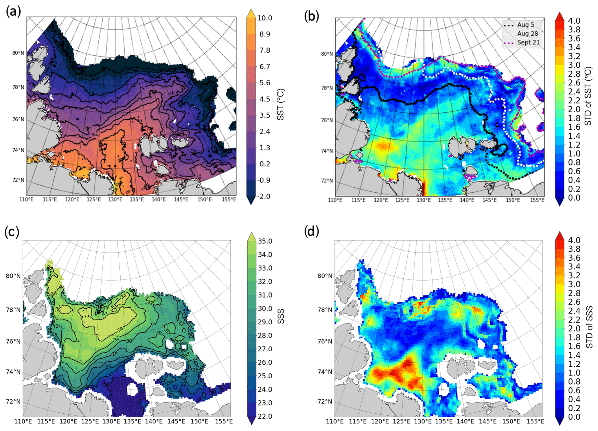
Figure 6Mean DMI SST (a) with its SD (b) and mean SMOS SSS (c) with its SD (d) for August–September 2018. The dotted lines in (b) show the position of the sea ice edge at different moments of time before and during the ARKTIKA-2018 cruise.
3.1 Overview of SST and SSS in the Laptev and East Siberian seas in August–September 2018
The mean SST during the 2 summer months is 2.18 ∘C in the Laptev Sea (between the Severnaya Zemlya Archipelago and the new Siberian islands), and 1.13 ∘C in the part of the East-Siberian Sea investigated (Fig. 6). The highest temperatures (above 6 ∘C, up to 9 ∘C) were observed close to the Lena River delta in Yanskiy Bay and in Olenekskiy Bay in front of the Khatanga River. A warm water pool associated with the river plume between 125 and 135∘ E progressively propagates northeastward and warms up this part of the sea: 0 ∘C isotherm at 140∘ E meridian is situated 100 km northward compared to its position at 120∘ E. The studied part of western East Siberian Sea was not completely ice-free in August–September 2018. Negative temperatures are observed near the ice edge at a distance of 50–100 km of the ice edge almost everywhere, except for a small area at 80∘ N, 160∘ E, where warm river water meets the sea ice with no open water with negative temperatures. The strongest gradients are observed along the sea ice edge and the river water plume (up to 0.05 ∘C km−1). Standard deviation of SST in Fig. 6 is the largest in Olenekskiy Bay (over 2.5 ∘C), along the coastline close to the Khatanga estuary (2.5–3 ∘C), the Lena River delta (about 4 ∘C), and in marginal ice zone (mostly over 1.5 ∘C). The remarkable variation of SST in the central part of the Laptev Sea should be associated with the thermal front (largest SST gradients) displacement.
The averaged SSS is 28.75 (with uncertainty of 0.10) in the Laptev Sea and 27.74 (with uncertainty of 0.20) in the western East Siberian Sea (Fig. 6). The spatial distribution of mean salinity for August–September 2018 shows the freshest water (salinity below 20) within the river plume northeast of the Lena River delta and within the southern part of the East Siberian Sea. Water with salinity below 28 reaches the sea ice edge in the northeastern Laptev Sea. Additional fresher water from the Kara Sea enters via the Vilkitskiy and Shokalskiy straits in the west (salinity of 28–30) and is also observed along the sea ice edge, where it could be associated with ice melting. The most saline water (salinity above 34) is located in the central part of the Laptev Sea near 78–80∘ N, 120–140∘ E and in the northwest along the Severnaya Zemlya Archipelago. As also observed in SST, SSS in the Olenekskiy Bay is highly variable, which can be explained by the variation of the freshwater discharge during the 2 months. Nevertheless, large SSS variability is also observed all along the sea ice edge: at 78–80∘ N in the north and northwest and at the boundary between the Laptev and East Siberian seas. This large variability can be explained in two ways: physical (haline fronts related to sea ice melting) and instrumental (remaining ice contaminated pixels, lower sensitivity of L band in cold water). At 78–80∘ N, 125∘ E, free-floating patches of broken ice detached from compact sea ice edge are observed during several weeks in August–September 2018. Random pieces of broken sea ice are not always recognized by ice-mask filters, and thus they can artificially increase SSS variability. At the same time, this is the area where river water encounters sea ice, which induces natural variability.
3.2 Observed surface water masses of the Laptev Sea and their transformation
To generalize our understanding of vertical structure of the studied area, we use the classical T–S analysis, first based on CTD measurements. Figure 7 shows the temperature–salinity distributions in the upper 200 m, colored as a function of depth. The most prominent feature on the diagram is the transformed Atlantic Water mass with salinity close to 34.5–35, temperatures from −0.5 to 2.5 ∘C lying at a depth of 100–200 m. The water mass overlying the Atlantic Water (between 50 and 100 m depth) is the lower halocline water, described by Dmitrenko et al. (2012) as having salinity in a range 33–34.5, and negative temperatures starting from the lowest values presented in Fig. 7, −1.7 to 2.5 ∘C. The surface water observed in the upper 50 m is in general less saline (salinity below 34), but we can clearly observe two separate branches with negative and positive temperatures. The two upper-layer branches are (1) warmer ([−1; 6] ∘C) and low-saline (below 34) surface water of the ice-free Laptev Sea and (2) colder ([−2; 0] ∘C) and low-saline waters of the ice-covered East Siberian Sea. The latter corresponds to the measurements from the transects 7 and 8 eastward of 150∘ E.
It should be remembered that a T–S diagram based only on CTD measurements does not provide an instantaneous view on the ocean state but is a collection of conditions encountered in different regions at different times (from the end of August to the end of September 2018). During the summer months, the surface water of the Arctic Ocean quickly evolves, and the synoptic satellite data provide an additional information to the point-wise in situ measurements.
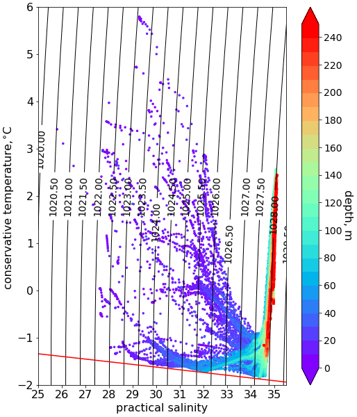
Figure 7T–S diagram based on the CTD data in the upper 250 m, color coded by depth. The red line shows the freezing line.
Using DMI SST and SMOS SSS weekly estimates, we plotted T–S diagrams similar to the one in Fig. 7, but only for surface satellite measurements for several reference days: 1, 15, 30 August, 4, 13, and 30 September 2018 (Fig. 8). On the lower row, we present all in situ measurements in the upper 6.5 m and the differences between satellite-derived sea surface temperature and salinity for the selected day. The range of variation in SSS and SST values covered by the satellite measurements (first row of Fig. 8) is an order of magnitude wider than the one covered by in situ measurements (Fig. 8, first column, bottom row). The difference in T–S diagrams covered by each type of measurement cannot be explained by the errors of satellite measurements (rms difference with respect to in situ measurements of 0.77 ∘C and 0.8 in temperature and salinity, respectively) or by the uncertainties associated with each satellite product (Figs. 4b and 5b). It primarily reflects the much more extensive spatiotemporal monitoring of different water masses by satellite measurements, e.g., the in situ measurements miss the southern Laptev sea, close to the origin of the riverine water. The DMI SST increases only up to the end of August with the maximum temperatures from 8 to 11.5 ∘C in some cases and then decreases to 4.5 ∘C by the end of September. The temperature changes by 0.5–1 ∘C per week (while increasing and decreasing).
Based on the Fig. 8 visual analysis, we propose identifying 6 surface water masses in the Laptev and East Siberian seas (Table 1) to follow the transformation of surface waters during 2 summer months (Fig. 9). The number and the limits of water masses were arbitrarily chosen based on the temperature–salinity scatterplot for 4 September 2018, as this day allows us to separate the cores of surface waters into groups in the best way based on the density of points. The temperature and salinity ranges of variation of each class are also well above the T and S uncertainties.
The main surface water masses are warm and fresh (WF) river water and cold and saline (CS) open sea water. All other water masses show either different stages of transformation of these two water masses or are advected from other regions. It should be noted that satellite-derived data have a larger range of temperature and salinity than the near-surface (upper 6.5 m) in situ measurements, which enables this detailed classification. The locations of the different water masses for specific days are shown in Fig. 9 together with the percentage distribution of water masses (the whole studied area is 100 %, and sea ice occupies some part of it).
On 1 August, the sea ice still covers more than 80 % of the studied area and extends on average to 78∘ N in the Laptev Sea, while the East Siberian Sea is almost completely covered by ice. WF river water is easily observable in the southern parts between 74 and 76∘ N. It occupies almost the same amount of surface as the CS, the rest of the open area is occupied by a transformed river water (warm and medium salinity, WMS; cold and medium salinity, CMS), which already formed a recognizable river plume front: its signature is continuous from 115 to 150∘ E up to the northern position of sea ice edge.
During the next 2 weeks the ice cover retreats, and a CF mass appears in the southwestern East Siberian Sea. The amount of this water increased progressively in this area during the remaining period. We suggest that this water mass represents the river water trapped under the ice and then exposed (see results of geochemical analysis below in Sect. 3.3.4).
On the 15 August, a water mass CMS also appears close to the Vilkitskiy Strait. It is less pronounced by the end of August, but a thin stream of cooled and transformed river water from the Kara Sea extends along the Taimyr peninsula in September. The Lena River water mixing and cooling also happens close to the sea ice edge in the northeastern Kara Sea. As a whole, the surface occupied by this water mass is steadily growing during the observed period to reach nearly 10 % of the surface by the end of September. We suggest that water mass CMS is a transformed version of water mass CF.
The end of August is warmer, as seen in Fig. 9; saline water with temperatures above 3 ∘C (water mass WS) occupies the central and the western part of the Laptev Sea (almost 10 % of the studied area). This water mass disappears by the end of September with the seasonal decrease of temperature.
By 13 September, the SST and SSS variability diminishes. The water mass CF in the northeastern Laptev Sea, consisting of cold fresh water, becomes saltier (and transforms into the water mass CMS). The freshwater cools south of the New Siberian islands and by September 25 occupies all the ice-free area. The river plume signature shifts to the New Siberian islands as well (Fig. 9). Cold and saline water dominates the surface of the Laptev Sea. Finally, by 25 September, the T–S diagram shows that most of the SSS and SST points lay between 25 and 35 and −1 and 4 ∘C, respectively, with a main core within a salinity range 25–35 and temperature between −1 to 1 ∘C and a second core within the salinity range 22.5–30 and temperature of 3–4 ∘C. The Laptev and the East Siberian seas then start to refreeze the most rapidly in the areas with cold and fresh river water.
Table 1The temperature and salinity of six defined surface water masses of the Laptev Sea using satellite data (see the text for the explanation of water masses names).
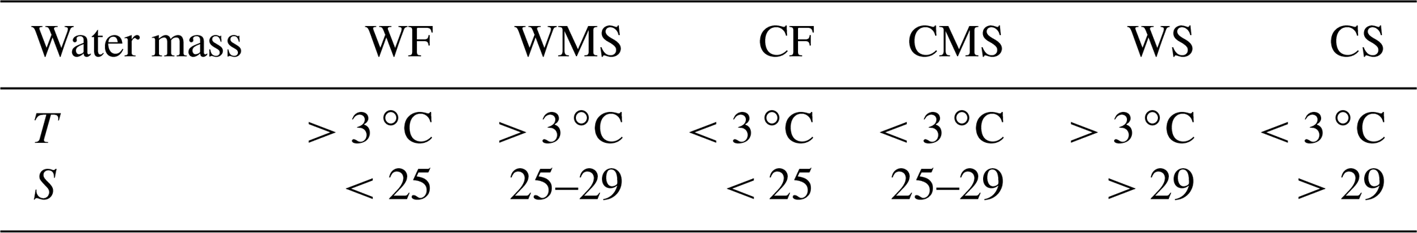
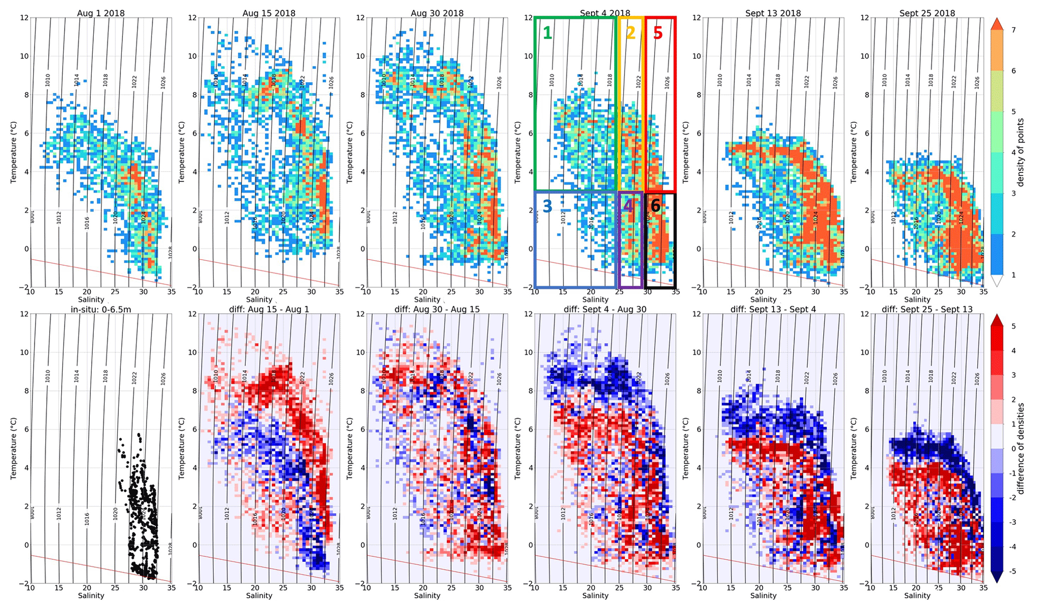
Figure 8Temporal evolution of surface water masses in August–September 2018 for the following reference days (upper row): 1, 15, 30 August, 4, 13, and 30 September 2018. color represents the density of points (number of observations with this temperature and salinity). The red line shows the freezing point temperature for different salinity. The boxes show the cores of six water masses described in text: 1 – WF, 2 – WMS, 3 – CF, 4 – CMS, 5 – WS, and 6 – CS. The lower row shows the T–S diagram based on CTD measurements in the upper 6.5 m only in column 1, and from column 2 to 6 the differences (in density points) between the reference days are shown.
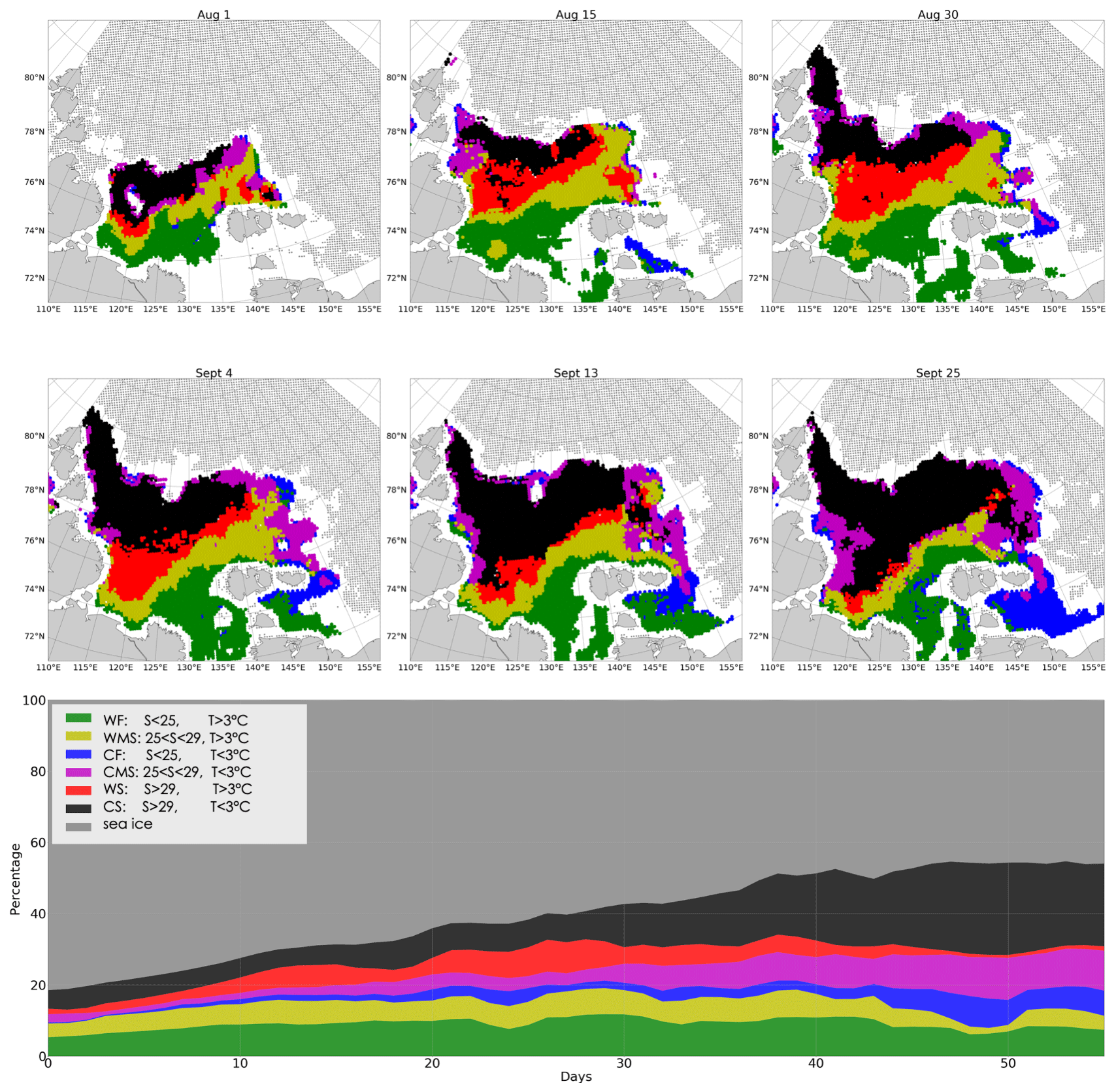
Figure 9Spatial distribution of surface water masses in August–September 2018. The upper row shows 1, 15, 30 August, and the middle row shows 4, 13, 30 September. Sea ice cover from AMSR2 is plotted as the dashed area. The lowest panel shows the temporal evolution of surfaces occupied by each water mass or sea ice cover in the Laptev Sea (in percentage of the Laptev Sea surface).
3.3 Freshwater variability in the Laptev Sea
To evaluate the distribution of freshwater input in the Laptev Sea in August–September 2018, we consider zonal and meridional transects along 78∘ N, 126∘ E and plot the temporal evolution of DMI SST, SMOS SSS “A”, wind speed, and SLP in Hovmöller diagrams. The freshwater can be defined by comparison to the saline “marine water” (typically 34.80, as in Aagaard and Carmack, 1989, or 34.92, as in Bauch and Cherniavskaia, 2018). As zero-salinity river water quickly mixes with a saltier marine water, in reality the “freshwater” is more “brackish” than “fresh”. Nevertheless, assuming a river plume front at the 29 isohaline for simplicity, the “freshwater” corresponds to all water masses with the salinity lower than 29, as we mentioned in Sect. 3.2.
3.3.1 Water from the Lena River plume
The zonal transect helps to investigate the mean stream position of the river plume away from the coast, in the central part of the Laptev Sea with more complex topography (Fig. 10). This virtual transect does not correspond to any real CTD transect, apart from some TSG profiles following the ship's route (see the position of virtual transect on the SST and SSS maps in Fig. 10f–g). In the western part (up to 130 ∘ E), the transect is located roughly above the continental slope and then over the shelf (Fig. 10e). The river water displacement roughly follows that of sea ice edge in the east and is bounded by the shelf break in the west. Overall, temperatures are higher in August than in September: a warm pool with SST over 6 ∘C is observed during the first 30 d at 78∘ N, 130–147∘ E, with the highest temperatures on 26 August. These coordinates define the position of the river plume at 78∘ N latitude, as can be clearly seen in the salinity values varying in a range of 27–30. Relatively strong daily winds (10–12 m s−1) observed during the first 10 d of September were associated with a series of cyclones, which strongly impacted the surface layer: the median temperature over the zonal transect decreased from 3 ∘C to almost 0 ∘C, and salinity increased by 1. As the amount of incoming solar radiation diminishes in September, the maximum SST values did not exceed 3 ∘C anymore. Nevertheless, at the end of September, a new freshwater patch was observed at 140∘ E (less visible in SST field) indicating that the “upstream” surface mixed layer (in the southern part of the Laptev Sea) contained a sufficient amount of freshwater to restore its previous state after a mixing event induced by the wind. Another possible explanation is that a small peak observed in the Lena River discharge in the first days of September (Fig. 3) introduced an additional portion of freshwater that reached 78∘ N several weeks later.
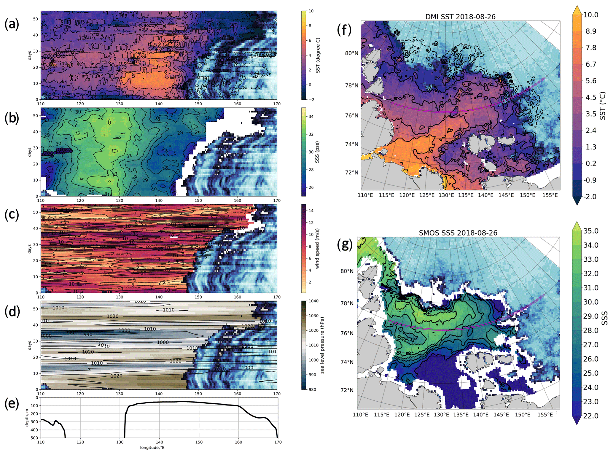
Figure 10Hovmöller diagram of DMI SST (a), SMOS SSS “A” (b), ASCAT wind speed (c), and ERA5 sea level pressure (d) for the zonal transect at 78∘ N. Small colored circles in the SST and SSS diagrams (a, b) show in situ measurements of temperature and salinity (first CTD or TSG at 6.5 m). Sea ice concentration (AMSR2) is indicated with a blue color; see Fig. 5 for the color scale. The bathymetry along the virtual transect (e) is extracted from “1 arcmin Global Relief Model” (Amante and Eakins, 2009). The position of a virtual transect is shown on DMI SST and SMOS SSS “A” maps for 3 September 2018 (f, g) with magenta lines.
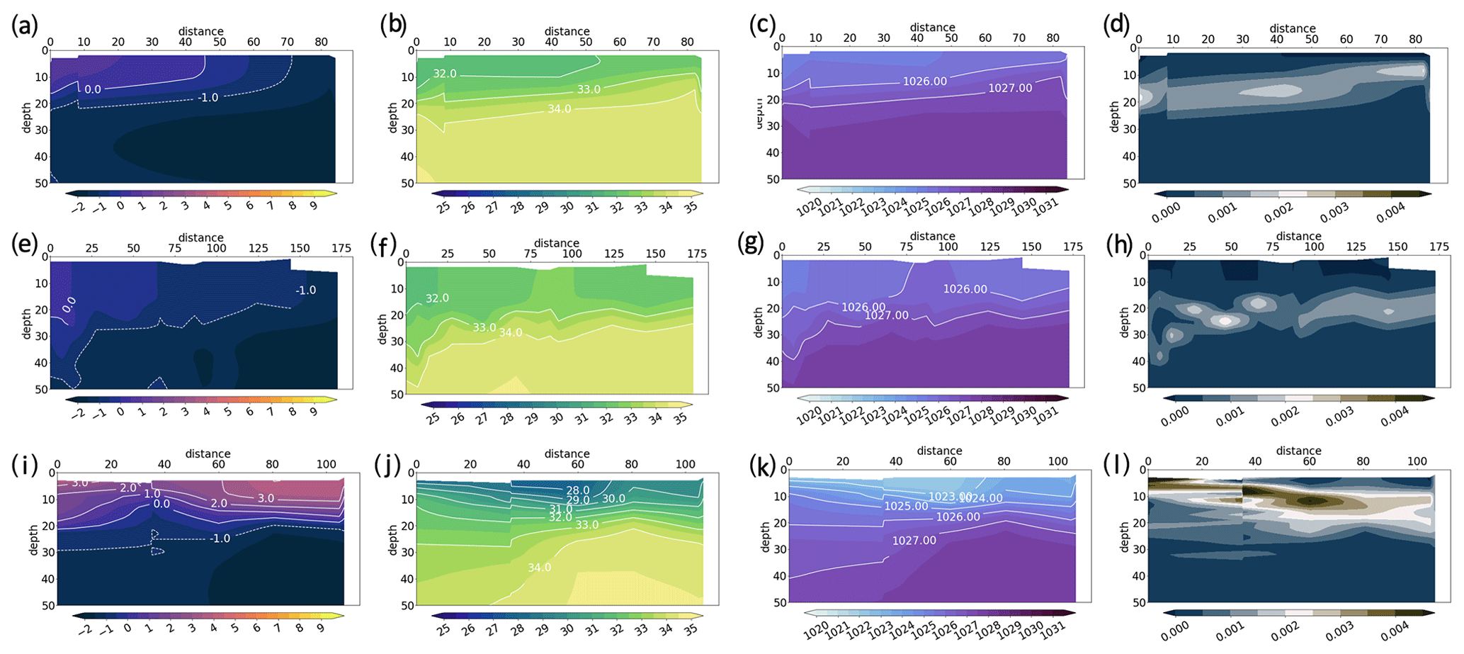
Figure 11Temperature (∘C; left, first column), salinity, (second column), water density (kg m−3; third column) and buoyancy frequency, (s−1; right, fourth column) obtained from CTD measurements in the upper 50 m for transect 1 northward of Arkticheskiy Cape (upper row), transect 10 across the Shokalskiy Strait (second row), and transect 4 across the Vilkitskiy Strait (lower row). See Fig. 1 for the transects' positions. The 0 km point is always placed at the southern point of each transect.
3.3.2 Water from the Kara Sea
The zonal transect allows us to see not only the Lena River plume but also the Kara water intrusions in the west. The selected zonal transect at 78∘ N is partly lying in the Vilkitskiy Strait connecting the Kara and the Laptev seas. Being a reservoir for two other great Siberian Rivers, the Ob and the Yenisei, the Kara Sea has a low salinity compared to the central Arctic Basin (Janout et al., 2015). In the absence of significant river sources on the Severnaya Zemlya Archipelago, we considered that the freshwater input close to the Vilkitskiy and the Shokalsky straits arrived from the Kara Sea.
We observe the freshwater arriving from the Kara Sea at 110–115∘ E with typical values of 25–28 during the first 20 d of August and at the end of September (Fig. 10b). It is noteworthy that the SST fields do not indicate the presence of these intrusions so clearly. This suggests that fresh and warm water of the Ob and Yenisei rivers arriving into the Laptev Sea have already lost a significant part of their heat content to the atmosphere but that the freshwater layer is not completely mixed with the surrounding sea environment.
In Fig. 11, the CTD data justify that the amount of freshwater arriving from the Kara Sea through the Vilkitskiy Strait is significantly greater than freshwater arriving via the narrow and rather shallow (250 m) Shokalskiy Strait between the Bolshevik and the October Revolution islands or north of the Severnaya Zemlya Archipelago at the traverse near the Arkticheskiy Cape across the continental slope. The temperature of the surface layer increases between 0 and 3.5 ∘C from north to south. Salinity transects indicate freshwater with salinity above 29 only in the Shokalskiy and the Vilkitskiy straits, which suggests very little advection of the Kara-origin freshwater via the north. From the buoyancy cross sections, we find that the strongest stratification is at 5–20 m depth, which corresponds to the 1024–1025 kg m−3 isopycnals depths. This result argues against a definition of freshwater content by the 1027.35 kg m−3 isopycnal of Polyakov et al. (2008), as the surface salinity and temperature in the Siberian shelf seas are lower than in other regions.
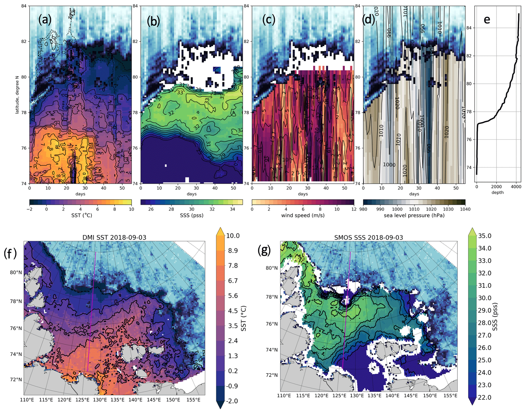
Figure 12Hovmöller diagram of DMI SST (a), SMOS SSS “A” (b), ASCAT wind speed (c), and ERA5 SLP (d) for the virtual meridional transect at 126∘ E. Sea ice concentration (AMSR2) is indicated with a blue color; see Fig. 5 for the color scale. The bathymetry along the transect (e) is extracted from “1 arcmin Global Relief Model” (Amante and Eakins, 2009). The position of a virtual transect is shown on SST SMI and SMOS SSS “A” maps for 26 August 2018 (f, g) with magenta lines.
3.3.3 Meridional transect
The meridional transect along 126∘ E (Fig. 12) partly corresponds to the standard oceanographic transect 5 carried out during ARKTIKA-2018 expedition on 1–4 September 2018 (Fig. 13). This transect helps to understand the northward propagation of the river plume and to evaluate the freshwater content using in situ data. The highest SST observed along 126∘ E longitude is 8 ∘C in August. Please note that a small cold temperature intrusion on days 22–26 probably corresponds to an error in DMI SST product due to a cyclone passage and thus either bad cloud masking or strong winds. This is an assumption reinforced when comparing DMI SST to SST AMSR2 microwave data (not shown here). More information on the SST corrections in the Arctic can be found in the work of Høyer et al. (2014).
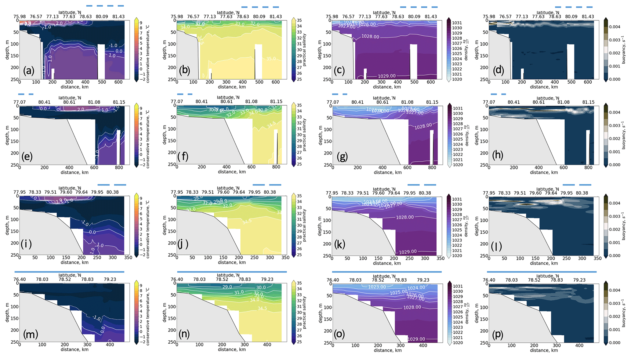
Figure 13Conservative temperature (left, first column), practical salinity (second column), density (third column), and Brünt–Vaisälä frequency (right, last column) in the upper 250 m along oceanographic transect 5 (a–d), transect 6 (e–h), transect 8 (i–l), and transect 7 (m–p). See Fig. 1 for the section positions. The 0 km point is always placed at the southern point of each transect. The dashed blue line indicates the MIZ for transects 5, 6, and 8 (the rest is ice-free area); the full line indicated that transect 7 was done under the ice.
The warmest (5–9 ∘C) and freshest (salinity of 20–30) water of river plume occupies the area between 74–77∘ N in August and progressively retreats in September: SST and SSS gradients become wider and less pronounced, temperature decreases to 3–4 ∘C. High wind speed (10–12 m s−1) associated with an atmospheric cyclone passage during the first two weeks of September is found both on the meridional and the zonal Hovmöller diagrams and might explain this widening of the surface thermal and haline frontal area. Nevertheless, a point-wise cross-correlation between the time series of wind speed and temperature or wind speed and salinity does not give statistically significant results: both correlation coefficients are below 0.2 at any time lag (0–10 d). Better correlation is observed with sea level pressure (up to 0.6 at some points), but over the 56 d investigated it is not statistically representative, as only two passing cyclones were observed.
The oceanographic transects allow us to estimate the thickness of the freshwater layer and how far the river water propagates under the ice. Transect 5 provides complementary information to the meridional Hovmöller diagram (Fig. 13, upper row) as it was done along the same 126∘ E parallel from 76 to 81.4∘ N on 1–4 September 2018. This date corresponds to the passage of several cyclones over the Laptev Sea, which, in turn, displaced the river front to the south, unfortunately, almost away from this oceanographic transect. Nevertheless, at 76–78∘ N (first 200 km of the transect), low salinity between 29–33 was still observed in the upper 25 m. A thin upper layer with positive temperatures has the same thickness but extends further northward up to 79∘ N. In the northern part of the transect, under the ice, the temperatures are below 0 ∘C and salinity is rather low (below 32). The low salinity under the ice suggests that the remnants of the river water arrived in this area earlier. If the river water was propagating under the ice when the Laptev Sea was not yet completely open, we should assume further mixing with sea water when the sea started to open in its central part (mixed water with salinity between 30 and 32 and still positive temperatures). The heat exchange with the sea ice might be more effective than with the atmosphere, so under the ice the temperatures are negative, and the warm river water signal is not observed anymore, contrary to salinity. At the same time, it depends on thermal conductivity in the ice, and its initial temperature profile, so this question needs further attention.
Overall, the first 150 km over the shelf, where the warmest and freshest water were observed, are characterized by the strongest stratification in the upper 25 m layer. This is the depth of a stable stratification for the whole transect, though stratification is less pronounced in the deeper part of the sea than over the shelf. Below the pycnocline, we observe cold (with negative temperatures) and saline (salinity between 33 and 34.5) water mass. The warm (T above 0 ∘C, following Pnyushkov et al., 2018) and saline (S above 34) Atlantic Water spreading along the continental shelf is best identified in temperature vertical profiles at 100–120 m depth but is also detected by the instability signal (right column in Fig. 13). The propagation of the Atlantic Water is beyond the scope of this paper, and though Atlantic Water is observed in all oceanographic transets presented below, it will not be discussed further here.
When considering other meridional transects (transects 6, 8, and 7 according to their positions), we follow the eastward propagation of the river water away from the Lena River delta. Transect 6 started on 5 September in the vicinity of the marginal ice zone in the deep northeastern part of the Laptev Sea and ended in the ice-covered part of the East Siberian Sea over the shelf on 9 September. This transect is not exactly perpendicular to the continental slope, so we cannot estimate the width of the river water plume, but overall the thickness of the upper layer is similar (20–30 m) to that observed with transect 5 in the deep part of the transect. The waters over the shallowest part (depth smaller than 60 m) were observed under the ice, as is clearly seen in the temperature signal that is negative even close to the surface. At the same time, the main freshwater core with the highest temperature is observed above the shelf break. The second core is observed in the northern part of the transect, with lower salinity than in the north of transect 5. The mixing over the shelf was effective enough to stretch the isopycnals between the bottom and the surface. Nevertheless, the depth of the maximum stratification is close to 20 m as for the shallow part of the transect 5. Over the edge of the continental slope, the maximum Brünt–Väisälä frequency moved deeper to 25 m, and over the deep-water part it moved to 30 m depth.
Transect 8 started on 15 September in MIZ over the deep part of the East Siberian Sea and finished by 17 September in the ice-free area over the shelf. The river signal is still very pronounced both in temperature and in salinity profiles, with an efficient mixing over the 60 m layer on the shelf and more concentrated isopycnals over the shelf edge. The most eastern transect 7 was conducted under the ice. The temperatures are thus negative above the Atlantic Water, but the salinity profile reveals the river water presence with the freshwater core as having a salinity below 29. The maximum value of Brünt-Väisälä frequency are less than for other transects and are observed at 20 m depth and at 55 m depth, following 1024 and 1026.5 kg m−3 isopycnals, accordingly showing the maximum stability of water vertical stratification under the ice.
To summarize, during summer 2018, we observe a northeastern displacement of the Lena River water, including in the MIZ and ice-covered area. We suggest that the active displacement started in the ice-covered conditions after the maximum of river discharge in June–July (following the Papa et al., 2008, study and the Lena River discharge measurements presented in Fig. 3), then, with progressive opening, part of the river water was mixed within the upper sea layer and exchanged heat with the atmosphere. For the water under the ice, the heat flux from the river water to the sea ice resulted in cooling of this water to the ambient negative temperature, but, at the same time, the sea ice protected the freshwater layer from wind-induced mixing, and thus it conserved a pronounced salinity signal.
3.3.4 Tracing surface water origin using oxygen isotopes (δ-O18)
The oxygen isotopes are considered a “natural tracer of river runoff in the Arctic Ocean” (Ekwurzel et al., 2001) and are widely used to detect the origin of water masses (Ekwurzel et al., 2001; Serreze et al., 2006; Bauch and Cherniavskaia, 2018). The simplest approach to detect a river water fraction in a water sample is to compute a ratio between the measured salinity and oxygen isotope 18 (δ-O18). As is described in Sect. 2, we used only the surface measurements in the upper 3 m layer.
Using a rather simple three-component model to distinguish the marine water, the river water (meteoric water), and the sea ice melt water described in Bauch and Cherniavskaia (2018), we calculated the fractions of each water mass (Fig. 14). In the work of Bauch and Cherniavskaia (2018), authors provide values of end-members of this model (typical salinity for each water mass and typical δ-O18 concentrations), so after resolving a simple system of three linear equations using the values of the total (measured) salinity and the measured δ-O18 concentration, we found a contribution of each fraction. As done in Bauch and Cherniavskaia (2018), the role of precipitation is neglected in this model, as its amount is insignificant compared to the river water input. The sea ice melt fraction can be negative in case of sea ice formation.

Figure 14Fractions of river water (a), sea ice melt water (b), and marine water (c), calculated using δ-O18 measurements and the Bauch and Cherniavskaia (2018) three-component model of freshwater balance. A thin black line shows the position of sea ice edge on 31 August 2018, when the northern stations of the meridional (5) transect along 126∘ E were done in the MIZ, and the blue line shows the sea ice edge on 16 September 2020, when the ARKTIKA-2018 expedition was working in the MIZ of the East-Siberian Sea. Please note that the color bar scale is different for each water fraction.
This analysis indicates that the most important fraction of river water is brought over the shelf and the shelf edge of the East Siberian Sea (Fig. 14a). At the same time, the water samples at the northern part of the 126∘ E transect consist of 10 %–15 % of the river water and only of 0 %–5 % of the sea ice melt fraction. Knowing that the main maximum of the river discharge occurs in June (Fig. 3), this fact supports our hypothesis that a noticeable amount of river water was distributed under the ice far northward into the deep part of the Laptev Sea (north of 80.5∘ N), where it will enter the central Arctic Basin later.
It is interesting that the areas with the highest sea ice melt fraction (Fig. 14b) (5 %–10 %) very slowly follow the sea edge, so they were observed in the central and western part of the Laptev sea and in the MIZ area in the East Siberian Sea. The sea ice formation (the negative values of sea ice melt fraction) is found in MIZ and its vicinity at 78–70∘ N, 150–160∘ E of the East Siberian Sea, which is expected as these measurements were done in the second part of September 2018, the beginning of freezing season. The presence of river waters may accelerate the sea ice formation if the air temperature favors it.
The surface water samples of the western and central parts of the Laptev Sea consist of large marine water fraction (90 %–95 %), Fig. 14c. The lowest marine water fraction (75 %–80 %) was found over a very shallow ice-free area between the New Siberian Islands and MIZ in the East Siberian Sea, where both sea ice melt and river water fractions are relatively high (5 %–10 % and 10 %–25 % respectively). Actually, it is the area of the most intense surface mixing that was observed using in situ measurements during the ARKTIKA-2018 expedition.
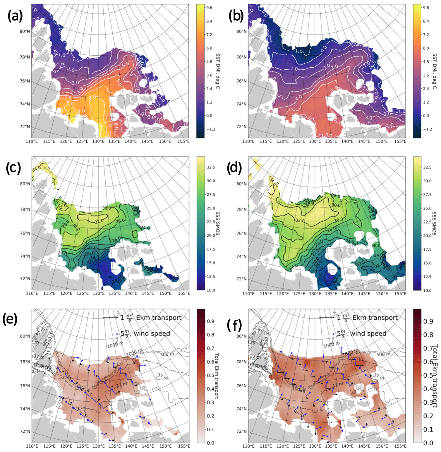
Figure 15August (left column) and September (right column) monthly means of (a, b) SST (∘C) and (c, d) SSS. Panels (e, f) show wind speed (m s−1) and direction with blue arrows, horizontal Ekman transport (m3 s−1) with black arrows, and total horizontal Ekman transport is shown using color shading.
3.4 Wind forcing
A previous study in this region (Dmitrenko et al., 2005) claimed that the surface front displacement is mainly governed by the wind and atmospheric pressure centers. To investigate the role of the wind forcing at the synoptic scales, we compute mean monthly Ekman transport for August and September 2018 (Fig. 15). The calculation is described in Sect. 2.
The discussed displacement of the river plume extension in August and September is clearly seen in both SST and SSS mean monthly fields (Fig. 15 a, c and b, d, respectively). The most pronounced feature in the SST field is the drop of SST by 3 ∘C in the central and southern Laptev Sea. Salinification of the northern, central, and southwestern part is observed in August–September SSS fields. The average wind speeds are low to moderate during August and September, 3–7 m s−1 (Fig. 15e, f). The wind field in August is more homogeneous and velocities are slightly higher with an overall southeasterly direction; the Ekman transport pushes the river water out of the central part of the Laptev Sea favoring its propagation under the ice.
In September, the wind changes its main direction to southwesterly, which leads to river water trapped in the Yanskiy bay, still favoring the freshwater flux propagation under the ice but mostly going into the southern part of the East Siberian Sea. As it was shown in the work of Lentz and Helfrich (2002), the onshore Ekman transport will generate a coastal downwelling followed by an increase of the salinity over the far-field areas of the river plume and its further offshore entrainment.
Based on in situ and satellite measurements, we document the evolution of water masses during August and September in the Laptev and the East Siberian seas. Satellite DMI SST and SMOS SSS “A” estimates are cross-validated with CTD data and continuous TSG measurements rarely done in this region. For the first time, thanks to the new satellite-derived salinity field (SMOS SSS “A”), a vast range of in situ measurements, and results of geochemical analysis, we follow how the river water input is distributed and where it is stored in the Laptev and the East Siberian seas at a synoptic scale.
To investigate local surface water masses, we use a variation of a classical TS analysis from satellite measurements. It helps to define new surface water masses adapted for the eastern Arctic Ocean with a typically low salinity and discuss their transformation. As the validity of SMOS SSS was successfully demonstrated and as SMOS measurements are accessible from 2010 to the present, this technique could be applied for future studies of the surface water transformation on different timescales.
The transformation of fresh water mass from river inflow occurs very quickly during the Arctic summer, over a period of typically 1–2 weeks. Based on our observations, we suggest that wind-induced vertical mixing, a weaker river discharge, and a continuously decreasing radiative income impact the variability of surface water characteristics, as can be clearly observed at the beginning of September 2018.
Following the classification of coastal buoyancy flows described in Lentz and Helfrich (2002), the displacement of river waters over the Laptev Sea shelf can be regarded as a slope-controlled buoyant gravity current, where the buoyancy forces are acting on the water body together with the wind stress and the bottom friction over a large area of the slightly inclined shelf, and at some point the buoyancy flow detaches from the bottom at a distance Wα. The upwelling-favorable winds will induce the offshore Ekman transport and stretch the buoyancy plume over the shelf, while the “downwelling” (onshore) winds will cause a deepening of the isopycnals. A sequence of upwelling–downwelling events can cause a further entrainment and a possible detachment of the buoyant coastal plume to the northern part of the shelf, the continental slope, and the deepening part of the Laptev Sea or over the East Siberian Sea shelf.
The variability in freshwater and the energy sources therefore partly explains the seasonal variability of the buoyant plume. The first yearly maximum of river discharge occurs in May, after an opening of the sea ice. The second one occurs in the beginning of August. This warm and fresh river water is redistributed and transformed in the surface layer of the Laptev Sea during the month of August. After the passage of several cyclones in the beginning of September, there is no additional source of heat and fresh water that would maintain the variability of water masses. Overall, in September, the “cold and saline” water mass progressively occupies the ice-free surface of the Laptev Sea instead of other (“transformed”) water masses observed there in August. Sea ice growth starts in the end of September, whereas the sea surface is fully covered by sea ice only by November 2018. The autumn freezing begins only after the heat accumulated during the summer season is released to the atmosphere and the water temperature at the surface drops to the freezing point.
An overview of Horner-Devine et al. (2015) describes main mechanisms of the river plume mixing and transport at different distances from the estuary area. Our in situ and satellite data make it possible to mostly investigate the “far-field” area of the river plume, where the balance between the wind stress and the buoyancy is governing the propagation and mixing of the surface fresh water with the “ambient sea”. As mentioned above, the Ekman transport illustrates an important forcing for the freshwater displacement. As the theoretical Ekman depth is controlled mainly by the Coriolis parameter f and by viscosity, assuming that the viscosity is homogeneous in the south of the Laptev and East Siberian seas, the Ekman depth exceeds the depth of some of the shallowest areas (according to the Baumann et al., 2018, study in the same region the Ekman depth is Dekm=37 m; see the position of 37 m isobath in the Laptev Sea in Fig. 15). Thus, the calculated Ekman transport should be regarded as a theoretical concept illustrating possible mechanisms of horizontal transport and vertical mixing only in the central and northern areas, whereas over the shallower seas the dynamics will be more constrained by mixing and the direction of the Ekman currents relative to bathymetric contours.
During the first 10 d of August, the upwelling-favorable north winds (mostly anticyclonic atmospheric conditions) stretched the freshwater plume from the south to the central Laptev Sea up to 78∘ N. In the second part of August, the wind changed its direction to more westerly and downwelling favorable, and thus the buoyant plume of river waters was displaced parallel to the coastline in the East Siberian Sea. An entrainment of the buoyant plume is evidenced in the CTD-measurements of salinity in the Eastern Laptev Sea and in the East Siberian Sea (transects 6–8).
The wind situation in August was favorable for the extreme propagation of river water into the northeastern part of the Laptev Seam followed by a propagation into the East Siberian Sea in the MIZ and under the sea ice. The propagation of river water under the sea ice is apparent in the western part of the East Siberian Sea, where two branches with warm and fresh cores have been observed with in situ data (transect 6). These branches can be understood as a result of previous entrainments of the Lena River water after a sequence of upwelling–downwelling events, pushing and detaching them offshore. After the river water separated from the estuary, it followed the shelf keeping its freshwater core with salinity below 29 up to the East Siberian Sea.
A pathway of the low-salinity Kara Sea water is observed during several days of our study. The Kara Sea water propagates mostly through the Vilkitskiy Strait and partly through the Shokalskiy Strait, but no freshwater is found northward of the Severnaya Zemlya Archipelago. Propagating along the coastline (reminiscent of a Kelvin wave starting from the Ob and Yenisey estuary), the low-salinity Kara water enters the Oleneksiy Bay where it meets another freshwater flux from the Khatanga and the Lena rivers. The arrival of freshwater via the Vilkitsiy Strait was already studied using in situ data by Janout et al. (2015) and Janout et al. (2017). However, this is the first time this event has been observed from satellite salinity data, which provides a unique opportunity for a regular monitoring. The freshwater input from the glaciers and icebergs of the Severnaya Zemlya Archipelago should probably also be taken into account, but this is out of the scope of this study, and we have assumed the volume of this source of freshwater to be negligible compared to the volume of the incoming very fresh Kara Sea water.
At a larger scale, the observed spatial variability can also be explained by a positive (in April–October 2018) Arctic Oscillation index favoring the eastward propagation of fresh water, as has been demonstrated in studies by Morison et al. (2012), Armitage et al. (2016), and Armitage et al. (2018). An important part of the northward propagation to the shelf edge is not explained by the positive AO. Based on the oxygen isotopes results, we claim that a similar propagation of river water far northward happened before the observed period (in June–July), when the Laptev Sea was still covered with ice and the Lena River discharge was at its largest (Fig. 3). At the northern end of the 126∘ E transect, under the ice, the upper 25 m layer is fresher with a salinity below 33, which supports this hypothesis. There is no evidence that the sea ice melting itself created such a considerable layer of freshwater. Our isotopes estimates could be further refined using alkalinity to separate the meteoric water estimated with water isotopic analysis (river input from precipitation). A study by Bauch and Cherniavskaia (2018) also supports the influence of river water, as a similar situation was observed in 2011. Unfortunately, the present spatial resolution of satellite-derived SSS and its uncertainty due to the proximity of sea ice makes it difficult to separate river water from the freshening associated with sea ice melt. No accurate satellite measurement of sea ice thickness in the MIZ is available at present to the best of our knowledge, and hence it is not easy to evaluate the freshwater input due to the sea ice melting on the scale of several months. Nevertheless, the existing satellite data already have a great potential for the Arctic studies of fresh water. To improve this evaluation of the freshwater budget in the Arctic Ocean, we suggest that appropriate numerical models assimilate the estimates of river discharge, new satellite-derived sea surface salinity, and wind data. An attempt to analyze the new sea level dataset provided by DTU (Danish Technological University) for the Arctic Ocean (Andersen and Knudsen, 2009) and calculated geostrophic currents is discussed in the Appendix and enriches the overview of the surface ocean dynamics during the selected summer months. Nevertheless, at present it seems that additional work on the continuous absolute dynamic topography (ADT) estimates over the shallow water is needed to use this dataset for the studies of coastal flow variability.
We calculated two monthly fields of absolute dynamic topography and geostrophic currents from sea level anomalies (SLAs) Arctic L4 product and mean dynamic topography (MDT) provided by the Danish Technological University (Fig. A1, Andersen and Knudsen, 2009). Sea level anomalies are available as mean monthly values on a grid adapted to polar regions with 0.25∘ step for latitude and 0.5∘step for longitude. Mean dynamic topography global model with 1 min spatial resolution was used to compute ADT. The resulting monthly absolute dynamic topography () was calculated for selected summer months.
Overall, the ADT remarkably follows the ocean bottom topography, with higher SLA over the shelf and lower SLA over the deep part of the studied area, which corresponds to the study of Armitage et al. (2016). The only exception is negative SLA in Olenekskiy Bay in August 2018. We suggest that the general northward wind-induced displacement of the water over the very shallow southern part of the sea was compensated for only by the river water inflow to the east of 122∘ E, close to the Lena River delta. Positive SLAs were more pronounced in September than in August, though in August the SST was higher over the southern and central parts of the Laptev Sea, and the salinity was lower in Olenekskiy Bay. The importance of the steric component in variation of the sea level in August–September is thus doubtful, though several sources of uncertainty can impact the quality of these SLA data: uncertainties in the tidal model, the bathymetry precision, and the accuracy of the MDT over the shallow part of the Laptev Sea, etc., as Armitage et al. (2016) noticed in their work. It should be noted that sea surface height (SSH) variability of the Laptev and the East Siberian seas presented in the work of Armitage et al. (2016) had the lowest correlation with in situ gauge measurements in the Arctic Ocean because of the “seasonal runoff”.
The geostrophic currents were calculated following: , , where h is ADT and x and y are the distance in meters. Geostrophic currents presented in Fig. A1 are weak (0.1–1 cm s−1 with more intense zonal component) and demonstrate rather chaotic structures during the summer months of 2018. Among the well-pronounced features, we find an outflow from the Laptev Sea in the Vilkitskiy Strait. Above the continental slope edge, the principal direction of currents is westward with a maximum current speed of 0.5 m s−1. Further south, an outflow at 122 and 130∘ E contributes to transport the Lena River water into the central part of the Laptev Sea. In Yanskiy Bay a vortex-like system exists in both August and September 2018. Geostrophic currents in the East Siberian Sea were calculated from the altimetric measurements in MIZ and thus should be interpreted with care. Armitage et al. (2017) stated that the SSH measurements there cannot reflect the mesoscale phenomena, because of the small Rossby radius (on the order of 1 km) and the altimeter along-track resolution of 300 m. At the same time, the same study reported the largest eddy kinetic energy in the shallowest areas.
From our calculations, a cyclonic feature of 150 km in diameter is seen at 79∘ N, 157∘ E, which might be topographically induced, as well as a similar cyclonic feature at 78.5∘ N, 135∘ E. An extended study should be carried out to validate the accuracy of altimetry-derived currents in this region with mooring- or vessel-mounted acoustic Doppler current profiler (ADCP) measurements.
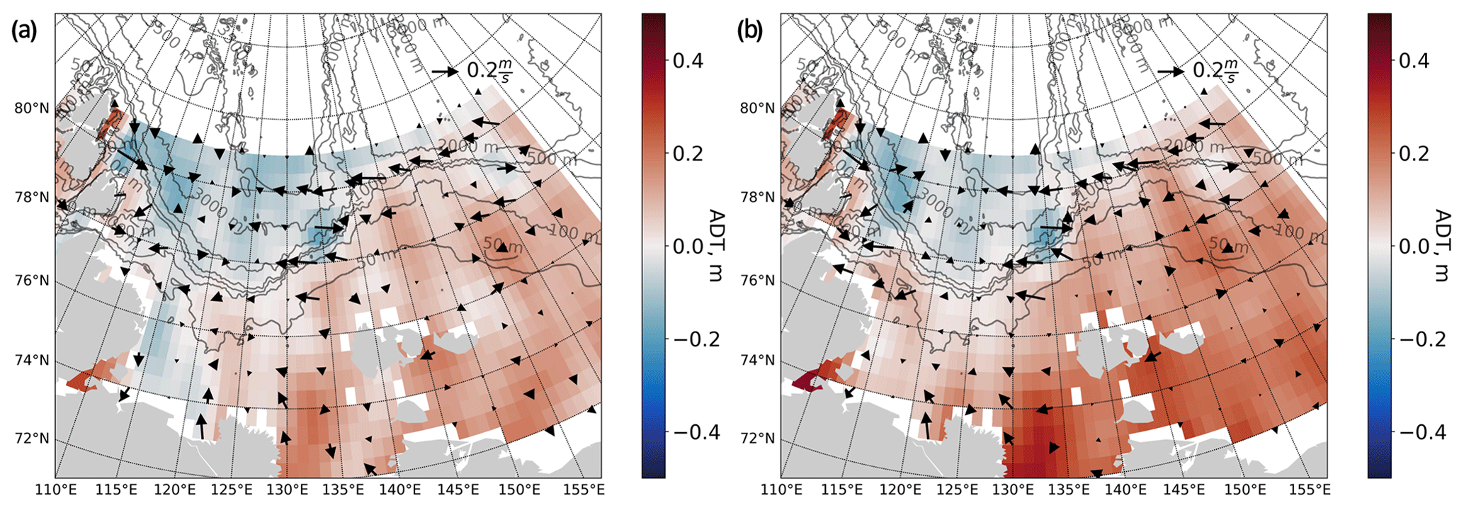
Figure A1Absolute dynamic topography (m) and geostrophic currents (m s−1) in August (a) and September (b) 2018, calculated from DTU monthly sea level anomaly.
In situ oceanographic measurements were prepared by Polyakov and Rember (2019, https://doi.org/10.18739/A2X34MS0V) and Alkire and Rember (2019, https://doi.org/10.18739/A2FX73Z1F). River discharge data were distributed by Shiklomanov et al. (2020, https://arcticgreatrivers.org/data/). DMI SST data were downloaded from https://resources.marine.copernicus.eu/?, last access: 24 January 2021. The SMOS SSS dataset is not distributed publicly as it was a work under development and was later published separately as an updated dataset. Sea ice concentrations from AMSR2 can be found at https://seaice.uni-bremen.de/data/amsr2/asi_daygrid_swath/ (last access: 24 January 2021) and sea ice charts at http://www.aari.ru/odata/_d0004.php (last access: 24 January 2021). Wind speed and directions were distributed by Ricciardulli et al. (2016, https://www.remss.com/missions/ascat). Sea level pressure comes from ERA5 hourly reanalysis https://cds.climate.copernicus.eu/cdsapp#!/dataset/reanalysis-era5-single-levels?tab=overview (last access: 24 January 2021).
AT and AS carried out the research. AT, NKT, VI, and MM did the data collection and interpretation. AS, JB, NK, and GR created the salinity dataset. AT wrote the paper with contributions from all co-authors. VI, BC, JT, JB, and GR defined the concept and methodology and supervised the study. JB and GR edited the manuscript.
The authors declare that they have no conflict of interest.
We thank Jean-Luc Vergely for fruitful discussions about SMOS SSS data filtering in the Arctic ocean. We thank Mattew Alkire, Andrey Novikhin, Natalia Vyazigina, the whole hydrochemistry team of the ARKTIKA-2018 expedition, and Ekaterina Chernyavskaya for the collection of water samples for the oxygen isotopes analysis, their analysis, and further discussion. We thank all the scientific team of the ARKTIKA-2018 expedition and the crew of RV Akademic Tryoshnikov for their work. This study was supported by the French CNES-TOSCA SMOS-OCEAN project. Anastasiia Tarasenko, Vladimir Ivanov, and Nikita Kusse-Tiuz acknowledge financial support from the Ministry of Science and Higher Education of the Russian Federation, project RFMEFI61617X0076.
Anastasiia Tarasenko, Vladimir Ivanov and Nikita Kusse-Tiuz acknowledge financial support from the Ministry of Science and Higher Education of the Russian Federation, project RFMEFI61617X0076, and Alexandre Supply, Jacqueline Boutin, and Gilles Reverdin acknowledge the French CNES-TOSCA SMOS-OCEAN project.
This paper was edited by John M. Huthnance and reviewed by four anonymous referees.
Aagaard, K. and Carmack, E. C.: The role of sea ice and other fresh water in the Arctic circulation, J. Geophys. Res.-Oceans, 94, 14485–14498, 1989. a, b
Alkire, M. and Rember, R.: Geochemical observations of seawater in the eastern Eurasian Basin, Arctic Ocean, 2018, https://doi.org/10.18739/A2FX73Z1F, 2019. a
Amante, C. and Eakins, B. W.: ETOPO1 Global Relief Model converted to PanMap layer format. NOAA-National Geophysical Data Center, PANGAEA, https://doi.org/10.1594/PANGAEA.769615, 2009. a, b, c
Andersen, O. B. and Johannessen, J. A.: The High Latitude Seas and Arctic Ocean, in: Satellite Altimetry Over Oceans and Land Surfaces, edited by: Stammer, D. and Cazenave, A., CRC Press, Boca Raton, 271–296, 2017. a
Andersen, O. B. and Knudsen, P.: The DNSC08 mean sea surface and mean dynamic topography, J. Geophys. Res., 114, C11001, https://doi.org/10.1029/2008JC005179, 2009. a, b
Arias, M. and Laboratories, S.-O. E. S.: L2OS v662 Reprocessing Report, SO-RP-ARG-GS-0109, available at: https://smos.argans.co.uk/docs/reports/SO-RP-ARG-GS-0109_L2OS_Reprocessing_Report_v2.6_170717.pdf (last access: 25 January 2021), 2017. a
Armitage, T. W., Bacon, S., Ridout, A. L., Thomas, S. F., Aksenov, Y., and Wingham, D. J.: Arctic sea surface height variability and change from satellite radar altimetry and GRACE, 2003–2014, J. Geophys. Res.-Oceans, 121, 4303–4322, 2016. a, b, c, d, e, f, g, h, i
Armitage, T. W. K., Bacon, S., Ridout, A. L., Petty, A. A., Wolbach, S., and Tsamados, M.: Arctic Ocean surface geostrophic circulation 2003–2014, The Cryosphere, 11, 1767–1780, https://doi.org/10.5194/tc-11-1767-2017, 2017. a, b
Armitage, T. W., Bacon, S., and Kwok, R.: Arctic sea level and surface circulation response to the Arctic Oscillation, Geophys. Res. Lett., 45, 6576–6584, 2018. a, b
Bauch, D. and Cherniavskaia, E.: Water mass classification on a highly variable arctic shelf region: Origin of Laptev sea water masses and implications for the nutrient budget, J. Geophys. Res.-Oceans, 123, 1896–1906, 2018. a, b, c, d, e, f, g, h, i
Baumann, T. M., Polyakov, I. V., Pnyushkov, A. V., Rember, R., Ivanov, V. V., Alkire, M. B., Goszczko, I., and Carmack, E. C.: On the seasonal cycles observed at the continental slope of the Eastern Eurasian Basin of the Arctic Ocean, J. Phys. Oceanogr., 48, 1451–1470, 2018. a
Bertino, L., Lisæter, K., and Scient, S.: The TOPAZ monitoring and prediction system for the Atlantic and Arctic Oceans, J. Oper. Oceanogr., 1, 15–18, 2008. a
Boutin, J., Vergely, J.-L., Marchand, S., d'Amico, F., Hasson, A., Kolodziejczyk, N., Reul, N., Reverdin, G., and Vialard, J.: New SMOS Sea Surface Salinity with reduced systematic errors and improved variability, Remote Sens. Environ., 214, 115–134, 2018. a
Carmack, E. C., Yamamoto-Kawai, M., Haine, T. W., Bacon, S., Bluhm, B. A., Lique, C., Melling, H., Polyakov, I. V., Straneo, F., Timmermans, M.-L., and Williams, W. J.: Freshwater and its role in the Arctic Marine System: Sources, disposition, storage, export, and physical and biogeochemical consequences in the Arctic and global oceans, J. Geophys. Res.-Biogeo., 121, 675–717, 2016. a, b, c, d, e, f, g, h, i, j
Castro, S. L., Emery, W. J., Wick, G. A., and Tandy, W.: Submesoscale Sea Surface Temperature Variability from UAV and Satellite Measurements, Remote Sensing, 9, 1089, https://doi.org/10.3390/rs9111089, 2017. a, b
Charette, M. A., Kipp, L. E., Jensen, L. T., et al.: The Transpolar Drift as a Source of Riverine and Shelf-Derived Trace Elements to the Central Arctic Ocean, J. Geophys. Res.-Oceans, 125, e2019JC015920, https://doi.org/10.1029/2019JC015920, 2020. a, b, c, d
Cherniavskaia, E. A., Sudakov, I., Golden, K. M., Strong, C., and Timokhov, L. A.: Observed winter salinity fields in the surface layer of the Arctic Ocean and statistical approaches to predicting large-scale anomalies and patterns, Ann. Glaciol., 59, 83–100, 2018. a
de Boyer Montégut, C., Madec, G., Fischer, A. S., Lazar, A., and Iudicone, D.: Mixed layer depth over the global ocean: An examination of profile data and a profile-based climatology, J. Geophys. Res.-Oceans, 109, C12003, https://doi.org/10.1029/2004JC002378, 2004. a, b, c, d
Dinnat, E. P., Le Vine, D., Boutin, J., Meissner, T., and Lagerloef, G.: Remote Sensing of Sea Surface Salinity: Comparison of Satellite and In Situ Observations and Impact of Retrieval Parameters, Remote Sensing, 11, 750, https://doi.org/10.3390/rs11070750, 2019. a, b
Dmitrenko, I., Kirillov, S., Eicken, H., and Markova, N.: Wind-driven summer surface hydrography of the eastern Siberian shelf, Geophys. Res. Lett., 32, L14613, https://doi.org/10.1029/2005GL023022, 2005. a, b
Dmitrenko, I. A., Kirillov, S. A., and Tremblay, L. B.: The long-term and interannual variability of summer fresh water storage over the eastern Siberian shelf: Implication for climatic change, J. Geophys. Res.-Oceans, 113, C03007, https://doi.org/10.1029/2007JC004304, 2008. a
Dmitrenko, I. A., Kirillov, S. A., Ivanov, V. V., Rudels, B., Serra, N., and Koldunov, N. V.: Modified halocline water over the Laptev Sea continental margin: Historical data analysis, J. Climate, 25, 5556–5565, 2012. a, b, c, d
Eastwood, S., Le Borgne, P., Péré, S., and Poulter, D.: Diurnal variability in sea surface temperature in the Arctic, Remote Sens. Environ., 115, 2594–2602, 2011. a
Ekwurzel, B., Schlosser, P., Mortlock, R. A., Fairbanks, R. G., and Swift, J. H.: River runoff, sea ice meltwater, and Pacific water distribution and mean residence times in the Arctic Ocean, J. Geophys. Res.-Oceans, 106, 9075–9092, 2001. a, b
Foreman, R. J. and Emeis, S.: Revisiting the definition of the drag coefficient in the marine atmospheric boundary layer, J. Phys. Oceanogr., 40, 2325–2332, 2010. a
Grodsky, S., Vandemark, D., and Feng, H.: Assessing Coastal SMAP Surface Salinity Accuracy and Its Application to Monitoring Gulf of Maine Circulation Dynamics, Remote Sensing, 10, 1232, https://doi.org/10.3390/rs10081232, 2018. a
Haine, T. W., Curry, B., Gerdes, R., Hansen, E., Karcher, M., Lee, C., Rudels, B., Spreen, G., de Steur, L., Stewart, K. D., and Woodgate, R.: Arctic freshwater export: Status, mechanisms, and prospects, Global Planet. Change, 125, 13–35, 2015. a, b
Horner-Devine, A. R., Hetland, R. D., and MacDonald, D. G.: Mixing and transport in coastal river plumes, Annu. Rev. Fluid Mech., 47, 569–594, 2015. a
Høyer, J. L., Le Borgne, P., and Eastwood, S.: A bias correction method for Arctic satellite sea surface temperature observations, Remote Sens. Environ., 146, 201–213, 2014. a, b, c
Ivanov, V.: Physical oceanography obtained from the water sampling bottle files collected during Akademik Tryoshnikov cruise AT2018 to the Arctic Ocean, PANGAEA, https://doi.org/10.1594/PANGAEA.905472, 2019. a
Ivanov, V., Varentsov, M., Matveeva, T., Repina, I., Artamonov, A., and Khavina, E.: Arctic Sea Ice Decline in the 2010s: The Increasing Role of the Ocean-Air Heat Exchange in the Late Summer, Atmosphere, 10, 184, https://doi.org/10.3390/atmos10040184, 2019. a
Janout, M. A., Aksenov, Y., Hölemann, J. A., Rabe, B., Schauer, U., Polyakov, I. V., Bacon, S., Coward, A. C., Karcher, M., Lenn, Y.-D., Kassens, H., and Timokhov, L.: Kara Sea freshwater transport through Vilkitsky Strait: Variability, forcing, and further pathways toward the western Arctic Ocean from a model and observations, J. Geophys. Res.-Oceans, 120, 4925–4944, 2015. a, b, c
Janout, M. A., Hölemann, J., Timokhov, L., Gutjahr, O., and Heinemann, G.: Circulation in the northwest L aptev S ea in the eastern A rctic O cean: Crossroads between S iberian R iver water, A tlantic water and polynya-formed dense water, J. Geophys. Res.-Oceans, 122, 6630–6647, 2017. a, b
Johnson, M. A. and Polyakov, I. V.: The Laptev Sea as a source for recent Arctic Ocean salinity changes, Geophys. Res. Lett., 28, 2017–2020, 2001. a, b
Klein, L. and Swift, C.: An improved model for the dielectric constant of sea water at microwave frequencies, IEEE J. Oceanic Eng., 2, 104–111, https://doi.org/10.1109/JOE.1977.1145319, 1977. a
Kolodziejczyk, N., Boutin, J., Vergely, J.-L., Marchand, S., Martin, N., and Reverdin, G.: Mitigation of systematic errors in SMOS sea surface salinity, Remote Sens. Environ., 180, 164–177, 2016. a
Lenn, Y.-D., Wiles, P., Torres-Valdes, S., Abrahamsen, E., Rippeth, T., Simpson, J., Bacon, S., Laxon, S., Polyakov, I., Ivanov, V., and Kirillov, S.: Vertical mixing at intermediate depths in the Arctic boundary current, Geophys. Res. Lett., 36, https://doi.org/10.1029/2008GL036792, 2009. a, b, c
Lenn, Y.-D., Rippeth, T. P., Old, C. P., Bacon, S., Polyakov, I., Ivanov, V., and Hölemann, J.: Intermittent intense turbulent mixing under ice in the Laptev Sea continental shelf, J. Phys. Oceanogr., 41, 531–547, 2011. a
Lentz, S.: The response of buoyant coastal plumes to upwelling-favorable winds, J. Phys. Oceanogr., 34, 2458–2469, 2004. a
Lentz, S. J. and Helfrich, K. R.: Buoyant gravity currents along a sloping bottom in a rotating fluid, JFM, 464, 251–278, 2002. a, b
McDougall, T., Feistel, R., Millero, F., Jackett, D., Wright, D., King, B., Marion, G., Chen, C., Spitzer, P., and Seitz, S.: The International Thermodynamic Equation Of Seawater 2010 (TEOS-10): Calculation and Use of Thermodynamic Properties, Global Ship-based Repeat Hydrography Manual, IOCCP Report No, 14, available at: http://www.scor-int.org/Publications/Thermodynamic_TEOS-10_Manual_GOSHIP_19Aug09.pdf (last access: 25 January 2021), 2009. a
Morison, J., Kwok, R., Peralta-Ferriz, C., Alkire, M., Rigor, I., Andersen, R., and Steele, M.: Changing arctic ocean freshwater pathways, Nature, 481, 66–70, 2012. a
Olmedo, E., Gabarró, C., González-Gambau, V., Martínez, J., Ballabrera-Poy, J., Turiel, A., Portabella, M., Fournier, S., and Lee, T.: Seven Years of SMOS Sea Surface Salinity at High Latitudes: Variability in Arctic and Sub-Arctic Regions, Remote Sensing, 10, 1772, https://doi.org/10.3390/rs10111772, 2018. a
Osadchiev, A., Izhitskiy, A., Zavialov, P. O., Kremenetskiy, V., Polukhin, A., Pelevin, V., and Toktamysova, Z.: Structure of the buoyant plume formed by Ob and Yenisei river discharge in the southern part of the Kara Sea during summer and autumn, J. Geophys. Res.-Oceans, 122, 5916–5935, 2017. a
Osadchiev, A., Pisareva, M., Spivak, E., Shchuka, S., and Semiletov, I.: Freshwater transport between the Kara, Laptev, and East-Siberian seas, Sci. Rep.-UK, 10, 1–14, 2020. a
Papa, F., Prigent, C., and Rossow, W. B.: Monitoring flood and discharge variations in the large Siberian rivers from a multi-satellite technique, Surv. Geophys., 29, 297–317, 2008. a, b, c
Pfirman, S., Bauch, D., and Gammelsrød, T.: The northern Barents Sea: water mass distribution and modification, Ameircan Geophysical Union, Washington, DC, USA, 1994. a, b
Pnyushkov, A. V., Polyakov, I. V., Ivanov, V. V., Aksenov, Y., Coward, A. C., Janout, M., and Rabe, B.: Structure and variability of the boundary current in the Eurasian Basin of the Arctic Ocean, Deep Sea Res. I, 101, 80–97, 2015. a
Pnyushkov, A. V., Polyakov, I. V., Rember, R., Ivanov, V. V., Alkire, M. B., Ashik, I. M., Baumann, T. M., Alekseev, G. V., and Sundfjord, A.: Heat, salt, and volume transports in the eastern Eurasian Basin of the Arctic Ocean from 2 years of mooring observations, Ocean Sci., 14, 1349–1371, 2018. a
Polyakov, I. and Rember, R.: Conductivity, Temperature, Pressure (CTD) measurements from cast data taken in the Eurasian and Makarov basins, Arctic Ocean, 2018, https://doi.org/10.18739/A2X34MS0V, 2019. a
Polyakov, I. V., Alexeev, V., Belchansky, G., Dmitrenko, I. A., Ivanov, V., Kirillov, S. A., Korablev, A., Steele, M., Timokhov, L. A., and Yashayaev, I.: Arctic Ocean freshwater changes over the past 100 years and their causes, J. Climate, 21, 364–384, 2008. a, b
Rabe, B., Karcher, M., Schauer, U., Toole, J. M., Krishfield, R. A., Pisarev, S., Kauker, F., Gerdes, R., and Kikuchi, T.: An assessment of Arctic Ocean freshwater content changes from the 1990s to the 2006–2008 period, Deep Sea Res. I, 58, 173–185, 2011. a
Ricciardulli, L. and Wentz, F. J.: Remote Sensing Systems ASCAT C-2015 Daily Ocean Vector Winds on 0.25 deg grid, Version 02.1, gridded binary files, Santa Rosa, CA: Remote Sensing Systems, available at: https://www.remss.com/missions/ascat (last access: 24 January 2021), 2016.
Ricker, R., Hendricks, S., Kaleschke, L., Tian-Kunze, X., King, J., and Haas, C.: A weekly Arctic sea-ice thickness data record from merged CryoSat-2 and SMOS satellite data, The Cryosphere, 11, 1607–1623, https://doi.org/10.5194/tc-11-1607-2017, 2017. a, b
Rippeth, T. P., Lincoln, B. J., Lenn, Y.-D., Green, J. M., Sundfjord, A., and Bacon, S.: Tide-mediated warming of Arctic halocline by Atlantic heat fluxes over rough topography, Nat. Geosci., 8, 191–194, 2015. a, b
Rudels, B., Jones, E. P., Schauer, U., and Eriksson, P.: Atlantic sources of the Arctic Ocean surface and halocline waters, Polar Res., 23, 181–208, 2004. a, b
Schlosser, P., Bauch, D., Fairbanks, R., and Bönisch, G.: Arctic river-runoff: mean residence time on the shelves and in the halocline, Deep Sea Res. I, 41, 1053–1068, 1994. a
Semiletov, I., Dudarev, O., Luchin, V., Charkin, A., Shin, K.-H., and Tanaka, N.: The East Siberian Sea as a transition zone between Pacific-derived waters and Arctic shelf waters, Geophys. Res. Lett., 32, L10614, https://doi.org/10.1029/2005GL022490, 2005. a, b
Serreze, M. C., Barrett, A. P., Slater, A. G., Woodgate, R. A., Aagaard, K., Lammers, R. B., Steele, M., Moritz, R., Meredith, M., and Lee, C. M.: The large-scale freshwater cycle of the Arctic, J. Geophys. Res.-Oceans, 111, C11010, https://doi.org/10.1029/2005JC003424, 2006. a
Shiklomanov, A. I., Holmes, R. M., McClelland, J. W., Tank, S. E., and Spencer, R. G. M.: Arctic Great Rivers Observatory, Discharge Dataset, Version 240121, available at: https://arcticgreatrivers.org/data/ (last access: 24 January 2021), 2020.
Spreen, G., Kaleschke, L., and Heygster, G.: Sea ice remote sensing using AMSR-E 89-GHz channels, J. Geophys. Res.-Oceans, 113, C02S03, https://doi.org/10.1029/2005JC003384, 2008. a
Supply, A., Boutin, J., Vergely, J.-L., Kolodziejczyk, N., Reverdin, G., Reul, N., and Tarasenko, A.: New insights into SMOS sea surface salinity retrievals in the Arctic Ocean, Remote Sens. Environ., 249, 112027, https://doi.org/10.1016/j.rse.2020.112027, 2020. a
Tang, W., Yueh, S., Yang, D., Fore, A., Hayashi, A., Lee, T., Fournier, S., and Holt, B.: The Potential and Challenges of Using Soil Moisture Active Passive (SMAP) Sea Surface Salinity to Monitor Arctic Ocean Freshwater Changes, Remote Sensing, 10, 869, https://doi.org/10.3390/rs10060869, 2018. a
Timmermans, M.-L., Cole, S., and Toole, J.: Horizontal density structure and restratification of the Arctic Ocean surface layer, J. Phys. Oceanogr., 42, 659–668, 2012. a, b, c
Timokhov, L. A. and Chernyavskaya, E. A.: Osobennosti sostoyaniya poverhnostnogo sloya arkticheskogo basseina v anomal'noe leto 2007, Arctic and Antarctic Problems, 83, 19–27, available at: http://www.aari.ru/misc/publicat/paa_arj_jour.php?idnum=148 (last access: 25 January 2021), 2009. a, b
Vivier, F., Hutchings, J. K., Kawaguchi, Y., Kikuchi, T., Morison, J. H., Lourenço, A., and Noguchi, T.: Sea ice melt onset associated with lead opening during the spring/summer transition near the North Pole, J. Geophys. Res.-Oceans, 121, 2499–2522, 2016. a, b, c
Waldteufel, P., Vergely, J.-L., and Cot, C.: A modified cardioid model for processing multiangular radiometric observations, IEEE T. Geosci. Remote, 42, 1059–1063, 2004. a
Yin, X., Boutin, J., and Spurgeon, P.: Biases Between Measured and Simulated SMOS Brightness Temperatures Over Ocean: Influence of Sun, IEEE J. Sel. Top. Appl., 6, 1341–1350, https://doi.org/10.1109/JSTARS.2013.2252602, 2013. a
“Level 4 product” means that several swath measurements were interpolated to achieve a regular resolution in time and space.
“Level 3” means a product resampled at a uniform temporal–spatial grid, different from a swath grid.
“Level 2” product means that a geophysical parameter, e.g., SSS, was computed at the swath grid.