the Creative Commons Attribution 4.0 License.
the Creative Commons Attribution 4.0 License.
 | 08 Nov 2021
Dynamics of fortnightly water level variations along a tide-dominated estuary with negligible river discharge
Erwan Garel
Ping Zhang
Observations indicate that the fortnightly fluctuations in the mean amplitude of water level increase in the upstream direction along the lower half of a tide-dominated estuary (the Guadiana Estuary), with negligible river discharge, but remain constant upstream. Analytical solutions reproducing the semi-diurnal wave propagation shows that this pattern results from reflection effects at the estuary head. The phase difference between velocity and elevation increases from the mouth to the head (where the wave has a standing nature) as the timing of high and low water levels come progressively closer to slack water. Thus, the tidal (flood–ebb) asymmetry in discharge is reduced in the upstream direction. It becomes negligible along the upper estuary half as the mean sea level remains constant despite increased friction due to wave shoaling. Observations of a flat mean water level along a significant portion of an upper estuary suggest a standing wave character and, thus, indicate significant reflection of the propagating semi-diurnal wave at the head. Details of the analytical model show that changes in the mean depth or length of semi-arid estuaries, in particular for macrotidal locations, affect the fortnightly tide amplitude and, thus, the upstream mass transport and inundation regime. This has significant potential impacts on the estuarine environment in terms of ecosystem management.
- Article
(5020 KB) - Full-text XML
- BibTeX
- EndNote


When averaged over a tidal cycle, the slope of the free surface elevation is generally not flat everywhere in an estuary. Several factors operating at distinct frequencies may be responsible for mean (or subtidal and tidally averaged) water level variations along the channel, such as the tide, freshwater inputs, local or remote atmospheric conditions (e.g. wind and air pressure), and various coastal ocean processes acting at the mouth (e.g. Aubrey and Speer, 1985; Gallo and Vinzon, 2005; Henrie and Valle-Levinson, 2014; Jay et al., 2015; Laurel-Castillo and Valle-Levinson, 2020; Matte et al., 2013; Ross and Sottolichio, 2016; Shetye and Vijith, 2013; Wong et al., 2009). At a fortnightly timescale, tide-dominated estuaries commonly feature relatively high and low mean water levels (MWLs) on spring and neap tides, respectively, in relation to the tidal forcing variability produced by the interaction of the semi-diurnal M2 and S2 tidal constituents (Aubrey and Speer, 1985). The resulting compound tide (MSf) has a 14.8 d period, which corresponds to the beat period between M2 and S2 (i.e. ω S2– ω M2 = ω MSf, where ω is the tidal frequency; Dworak and Gomez-Valdes, 2005; LeBlond and Mysak, 1978). The tidal potential also contains energy at the MSf frequency, but this energy source is usually weak and becomes negligible in the upper estuary (LeBlond, 1979). Water level oscillations with MSf period along estuaries are typically referred to as fortnightly tides.
Fortnightly tides have been mainly described at long tidal rivers affected by substantial freshwater inputs. Subtidal changes in water elevation at these systems can be of order 1 m at the upper reaches and may have, as such, significant effects on navigability and tidal inundation (e.g. Aubrey and Speer, 1985; Godin, 1999; Guo et al., 2015; Jay et al., 2015; Matte et al., 2014). MSf tides with large amplitude derive from the subtidal friction produced by the interaction between the river flow and the various tidal constituents (Buschman et al., 2009; Cai et al, 2016a; Jay and Flinchem, 1997; Sassi and Hoitink, 2013). The river discharge nonlinearly enhances the subtidal friction experienced by the barotropic tidal wave propagating upstream (Godin, 1985, 1999; Guo et al., 2015; Jay, 1991; Matte et al., 2013; Pan et al., 2018; Sassi and Hoitink, 2013). Due to its nonlinear dependence on water depth, the subtidal friction is greatest on spring tides and is, thus, balanced by the largest subtidal water level gradient landward; likewise, the gradient is smallest on neap tides when friction is comparatively weak. This is demonstrated by analytical derivations of the along-estuary momentum equation for tidal averaged conditions, which indicates that the water slope term is dominantly balanced by the friction term (e.g. Buschman et al., 2009; Cai et al., 2016a, 2019, 2014; LeBlond, 1978; Sassi and Hoitink, 2013). Thus, if the river discharge and mean sea level remain constant, the variation in the mean slope with tidal forcing causes subtidal water levels to be higher at spring tide than at neap tide. The friction-induced modulation in subtidal water levels allows transporting, for any tidal amplitude, of the same volume of riverine water seaward over the neap–spring cycle (Guo et al., 2015). At settings with extended intertidal areas, the lateral spreading of the flood tidal wave produces additional frictional asymmetries between spring and neap tides that may also contribute to the increase in the fortnightly tide amplitude in the upstream direction (Friedrichs and Aubrey, 1988).
Without significant river discharge, fluctuations in the subtidal friction generated by tidal contributions alone may also produce a fortnightly tide (Vignoli et al., 2003). This case concerns many worldwide estuaries, typically in semi-arid regions, where the river flow influence is not relevant compared to the tidal forcing – during a large part of the year, at least (e.g. Correia et al., 2020; Descroix et al., 2020; Dias et al., 2016; Frota et al., 2013; Garel and D'Alimonte, 2017; Lamontagne et al., 2016; Lopez et al., 2020; McCutcheon et al., 2019; Valle-Levinson and Schettini, 2016). Due to high freshwater demands for irrigation and other uses, semi-arid estuaries are under increasing stress worldwide from decreased freshwater inflows (Feng and Fu, 2013; Leblanc et al., 2012). As for tidal rivers, an accurate knowledge of the water level variations at semi-arid estuaries with ephemeral freshwater inflows is necessary for ecosystem and freshwater management and for hydrodynamic research (Hoitink and Jay, 2016; Jay et al., 2011; Pan and Lv, 2019). However, the dynamics of the fortnightly tide produced by tidal asymmetry alone have been poorly documented so far.
The present study proposes to make explicit the dynamics of fortnightly tides in estuaries where tidal motion is the main forcing. Subtidal water level observations in a semi-arid estuary with negligible freshwater discharge (the Guadiana Estuary) are compared with the outputs of analytical solutions considering a semi-diurnal tide of variable forcing amplitude propagating along a convergent channel. The specific objectives are to establish the tidal properties that control the development of the subtidal slope along the channel, to evaluate the effects of reflection at the head, and to explore MWL variations in function of the tidal forcing and estuary geometry. Overall, this research proposes, for the first time, an analytical tool for assessing the impacts of geometric changes (such as the mean depth or length of the estuary) on fortnightly water level variations in tide-dominated estuaries with negligible river discharge. The results shed new light on how fortnightly dynamics in water levels are generated due to imposed tidal forcing at the mouth and tidal wave reflection from the head of the estuary. Through estimates of the MWL along the estuary, the approach is specifically helpful for sustainable water resources management of ecosystems, especially in macrotidal estuaries. In Sect. 2, the development of a fortnightly tide as a result of the balance between friction and water slope is described analytically. The study site and collected data are presented in Sect. 3, along with the hydrodynamic model used to reproduce tidal wave properties. The observational results are presented in Sect. 4. The model results are presented and explored in Sect. 5 to elucidate and discuss the dynamics of the fortnightly tide and implications for estuarine environments. The main conclusions of this work are summarized in Sect. 6.
The subtidal water level slope along an estuarine channel produced by tidal effects can be derived from the 1D momentum equation as follows (e.g. Savenije, 2012):
where U is the cross-sectional average velocity, h is the water depth, Z is the water level fluctuation in relation to the tidally average water level, g is the gravitational acceleration, t is time, x is the longitudinal coordinate directed landward, and K is the Manning–Strickler friction coefficient.
Assuming a periodic variation in flow velocity, the integration of Eq. (1) over a tidal cycle leads to the following (Cai et al., 2014; Vignoli et al., 2003):
where the overbars denote a tidal average. The second contribution to the subtidal water level in Eq. (2) originates from the advective acceleration term, which is relatively small when compared to the first contribution induced by the residual frictional effect, as long as the Froude number is small (which is usually the case in estuaries, e.g. about 0.14 at the Guadiana Estuary; see also Cai et al., 2019).
Thus, Eq. (2) simply expresses a balance between the slope and friction. In several cases, the contribution of the time-variable depth is a second-order effect for the hydrodynamics (for instance, if the tidal amplitude is relatively small compared with the depth), but it can still be relevant for the subtidal water level. The total free surface elevation Z is the sum of its tidal average (responsible for the subtidal slope) and tidal wave height Zt, such as (t), where the function fZ describes the variation in Z with time, and ζ is the ratio of the tidal amplitude to the water depth. From a Taylor expansion of , assuming that ζ≪1, the frictional contribution to Eq. (2) can be rewritten as follows:
where the additional term in parentheses can be significant, depending on the relative phase difference between U and Z, i.e. the phase lead ϕ of the velocity with respect to the water level (van Rijn, 2011). The analysis of a simple case like a purely sinusoidal signal of frequency ω shows this feature clearly. If U=υcos(ωt), where υ is the tidal velocity amplitude, and fZ=cos(ωt−ϕ), then , but ), which is vanishing only for (with n being an integer number), i.e. for a standing wave. In the latter case, the peak of flow velocity occurs when the water level attains the mean sea level value both during the flood and the ebb phases (ebb discharge is equal to flood discharge) and the tidally averaged water level keeps constant and horizontal along the channel. By contrast, if the wave contains a significant progressive component, the additional term produces a residual slope as follows:
Equation (4) shows that a purely sinusoidal tidal wave may produce a residual slope even in the absence of freshwater discharge into the estuary. In this case, the residual slope relates to intratidal variations in the friction experienced by the wave for distinct tidal velocities (tidal stages). When the lag between elevation and velocity is significant, the peaks of ebb and flood velocities occur during low and high water stages, respectively. Thus, the frictional term yields larger dissipation during the ebb phase than during the flood phase; this implies that the free surface slope must increase to compensate for the dynamic imbalance in order to conserve a zero discharge. This mechanism is also stronger at spring than at neap tides, resulting in fortnightly fluctuations of the residual slope; these dynamics are the scope of the present study.
3.1 Study area and data collection
3.1.1 Study site overview
The Guadiana Estuary consists of a single channel that connects the Guadiana River to the Gulf of Cadiz at the southern border between Portugal and Spain (Fig. 1). The channel is 78 km long and broadly oriented north–south, with a cross-section width that reduces exponentially from 700 m at the mouth to 60 m at the head. The thalweg is generally between 4 and 8 m, with a mean depth of approximately 5.5 m (Garel, 2017).
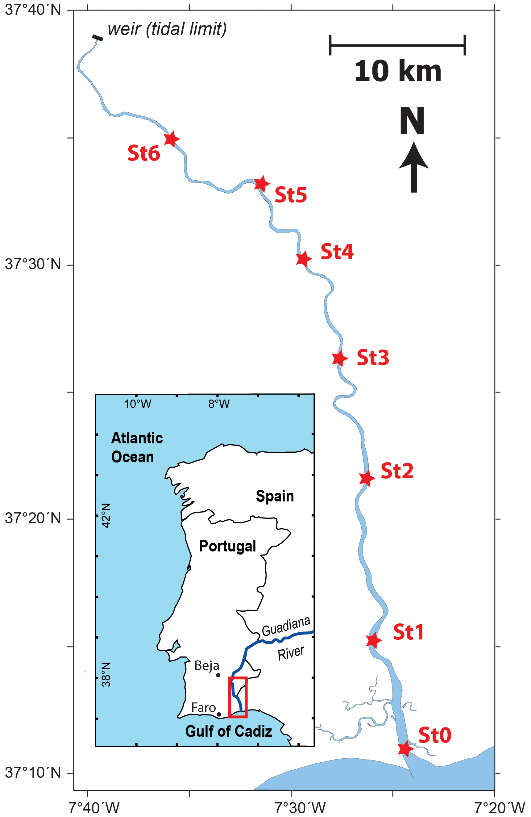
Figure 1Location of the pressure measurement stations along the Guadiana Estuary (St0–6; red stars) and the general location (inset).
Tides are semi-diurnal in the region, and their range falls in the microtidal to mesotidal regime (1.3 m during neaps and 2.6 m during springs, on average), with a maximum of 3.4 m. The amplitude of the dominant M2 constituent varies by <10 % along the estuary. It is slightly damped along the lower half of the estuary, where friction dominates morphological convergence effects, and it is slightly amplified along the upper half, due to reflection at the head which has the overall effect of reducing the friction experienced by the propagating wave (Garel and Cai, 2018).
The freshwater discharge into the estuary is generally low, in particular in summer when it is typically <10 m3 s−1 (see Garel and D'Alimonte, 2017). During a single tide, this rate corresponds to a volume of freshwater input approximately 70 times lower than the average tidal prism (30 Mm −3; Correia et al., 2020). Under these conditions, the water column is generally well mixed (Garel et al., 2009).
3.1.2 Data acquisition and processing
Water level variations along the Guadiana Estuary were measured from 31 July to 24 September 2015 with a series of seven pressure transducers (Level TROLL 700 Data Logger; In Situ), deployed every 10 km, approximately, from the mouth (St0) to 60 km upstream (St6; see Fig. 1). The sensor accuracy is rated at ± 0.55 cm by the manufacturer, and their maximum range is 11 m. During the survey period, the mean freshwater discharge was 7 m−3 s−1, and weather conditions were mild, typical of summers in the region. The largest spring and lowest neap tides were on 31 and 24 August 2015, with tidal ranges of 3.3 and 1.2 m, respectively.
The raw pressure data, recorded at 1 min intervals, were smoothed with a 5 min moving average window and resampled to a common time at a 10 min interval. The records were then corrected for atmospheric pressure variations obtained from a station (Faro) located 50 km westward from the mouth (see Fig. 1 inset). The mean value was removed from the corrected time series to obtain water level variations around zero at each station. Pressure differences between Faro and Beja, located 110 km northward (see Fig. 1 inset), were weak (< 2 mbar) during the survey, indicating an insignificant effect of meridional pressure variations on the water level slope along the estuary. It should be noted that the potential impacts induced by wind and waves on the water level dynamics during storms are not addressed since the study focuses on normal (fair) meteorological conditions.
Tidal amplitudes at each station were obtained through demodulation of the pressure records (see Garel and Cai, 2018). The resulting amplitudes were smoothed using a six-point moving average to discard jagged fluctuations induced by (small) diurnal inequalities of the astronomical tide. A continuous wavelet transform (CWT) analysis was performed to compare the amplitude of tidal species (diurnal D1, semi-diurnal D2, quarter-diurnal D4, and fortnightly Df) on the largest spring and lowest neap tides at each station. The basic principles of CWT analyses are described in Jay and Flinchem (1997; see their Eqs. 1–3).
A Butterworth low-pass filter with a cut-off period of 11 d was applied to the time series to expose the fortnightly modulation of water level variations (denoted hereafter as Zf). The low-pass filter was also applied with a 40 h cut-off period (discarding shorter periodic variations, which are mainly tidal) in order to assess the contribution of Zf to the obtained subtidal water level, Zs. The initial 4 d of the time series were discarded due to artefacts produced by the filtering process. Significant differences between Zs and Zf are produced by external agents (such as atmospheric or coastal ocean processes) operating (and affecting the surface water level) in the subtidal to fortnightly band period.
In estuaries, a consistent increase in the MWL in the upstream direction is also produced by the horizontal water density gradient (e.g. Savenije, 2012; Savenije and Veling, 2005). Neap–spring variations in the salinity intrusion length may, therefore, contribute to the observed fortnightly water level modulation (Zf). The effect of density on the slope was estimated based on CTD measurements performed every ∼4 km from the mouth to the freshwater front (defined as salinity <1 kg g m−3). These surveys were conducted at both high water slack (HWS) and low water slack (LWS) during consecutive spring (29 May 2018) and neap (6 June 2018) tides, with range of 2.5 and 1.1 m, respectively, under low river flow conditions (10 m3 s−1). The tidally averaged salinity curves were obtained as half the excursion length (Savenije, 2012). The contribution to the water level from the density effects (denoted as Zρ) was estimated as follows (e.g. Cai et al., 2016a, 2019; Vignoli et al., 2003):
where the axial distance x= 0 at the mouth, hm is the measured cross-sectional mean depth, and ρ is the (depth-averaged) water density. Hereafter, the subscript zero indicates a value at the mouth.
3.2 Hydrodynamic model of tidal wave propagation
To derive the analytical solution for tidal hydrodynamics along an estuarine channel, it is assumed that the tidally averaged cross-sectional area and width can be described by the following exponential functions (Savenije et al., 2008):
where a and b are the area and width convergence lengths, respectively. It is also assumed that the flow is concentrated in a rectangular cross section, with a possible influence from storage areas described by the storage width ratio rS that is defined as the ratio of the storage width BS to the tidally averaged width (). It directly follows from the assumption of a rectangular cross section that the tidally averaged depth is given by .
Toffolon and Savenije (2011) showed that the analytical solutions for tidal hydrodynamics along an estuary can be described by a few externally defined dimensionless parameters that depend on the estuary geometry and external forcing (see Table 1), i.e. the tidal amplitude ζ0, representing the boundary condition imposed at the estuary mouth, the estuary shape number γ, indicating the effect of the channel cross-sectional area convergence, the friction number χ0, describing the role of the frictional dissipation at the estuary mouth, and the dimensionless estuary length . In Table 1, η0 is the tidal amplitude at the mouth, c0 is the frictionless wave celerity in a prismatic channel (defined as ), and L0 is the frictionless tidal wavelength (). The tidal frequency of the considered constituent is (with T the tidal period). It is noted that the friction number χ0 is dependent on the Manning–Strickler friction coefficient K that describes the effective friction resulting from various environmental factors such as bedforms, grain roughness, vegetation, channel geometry (e.g. Savenije and Veling, 2005; Wang et al., 2014; Winterwerp and Wang, 2013), river discharge, and from nonlinear effects induced by minor tidal constituents (Prandle, 1997). The value of K is generally difficult to estimate accurately and is preferably obtained by calibrating the model results with observations, if available.
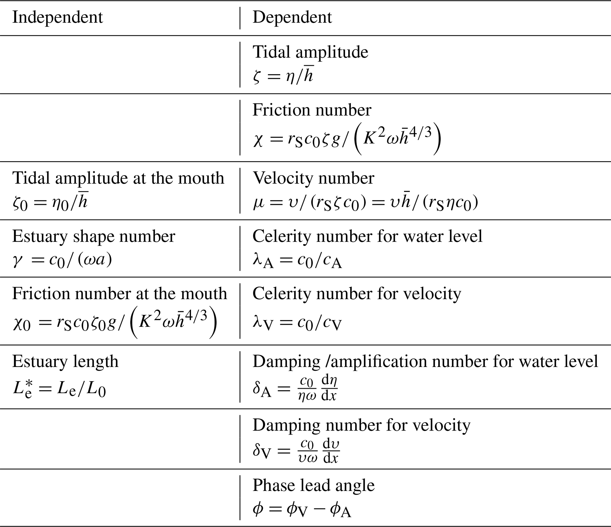
The corresponding dependent dimensionless parameters which are used to describe the main tidal hydrodynamics along the channel include the following (Table 1): the actual tidal amplitude ζ, the actual friction number χ (χ=0 in a frictionless case), the velocity number μ (the ratio of the actual velocity amplitude to the frictionless value in a prismatic channel), the celerity number for elevation λA and velocity λV (the ratio between the frictionless wave celerity in a prismatic channel and the actual wave celerity), the amplification number for elevation δA and velocity δV (describing the rate of increase, δA (or δV) >0, or decrease δA (or δV) < 0 of the wave amplitudes along the estuary axis), and the phase lead angle ϕ between velocity ϕV and elevation ϕA (ϕ= 90∘ for a standing wave).
The dependent parameters defined in Table 1 can be calculated using the equations developed by Toffolon and Savenije (2011; see also Cai et al., 2016b, and Eqs. 6–20 in Garel and Cai, 2018) for both infinite and semi-closed channels. To account for the longitudinal variation in the cross sections in width and depth, the entire channel was subdivided into multiple reaches. The solutions were then obtained by solving a set of linear equations, with internal boundary conditions at the junction of the sub-reaches satisfying the continuity conditions for both water level and discharge. Previous applications have shown that the model can accurately describe the effect of tidal forcing variations (e.g. spring and neap tides) on tidal properties along narrow convergent estuaries (such as the Guadiana Estuary) by considering a single effective tidal wave (Garel and Cai, 2018).
4.1 Fortnightly tide
Pressure records indicate large spring–neap fluctuations in tidal amplitude at the mouth (Fig. 2a), which are due to a relatively large S2 constituent in the region (Garel and Cai, 2018). At the mouth (St0), there is no apparent relation between the tidal amplitude and the (11 d) low-passed filtered water level, Zf. About 10 km upstream, at St1, Zf occasionally accompanied the tidal forcing variations, in particular during the tides on 24 (neap) and 31 (spring) August. Upstream (St2–6), Zf clearly co-varies, with the tidal amplitude (Fig. 2a, b) being relatively higher at spring tide and lower at neap tide (Fig. 2b, c), typical of a fortnightly tide (e.g. Buschman et al., 2009; Hoitink and Jay, 2016; Sassi and Hoitink, 2013; Speer and Aubrey, 1985). The greatest water level variations in Zf (about 20 cm in range) correspond to the largest changes in tidal height, observed between 24 and 31 August 2015 (see Fig. 2b). It is also noted that Zf at St1 is incongruous in September, showing variations that are unrelated to the signal at adjacent stations.
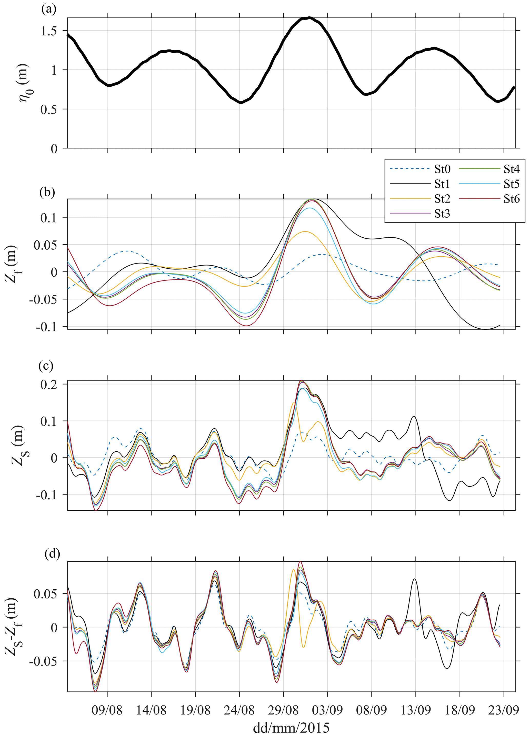
Figure 2(a) Tidal amplitude (η0, m) near the mouth (St0), (b) low-pass filtered (11 d) water level (Zf, m) at stations St0–6 along the estuary, (c) low-pass filtered (40 h) water level (Zs, m) at St0–6, and (d) residual water level Zs−Zf.
Linear correlations confirm that the tidal forcing and fortnightly water level modulations are not correlated at the mouth (Fig. 3a; blue line). The correlation increases significantly upstream until St3 (where the coefficient of correlation R is 0.8) and remains constant along the upper estuary half. Additionally, wavelet analyses show that, during the neap–spring tidal cycle on 24–31 August, the amplitude of the 15 d period species (Df) increased from about 0 cm at the mouth (St0) to 6 cm at St3 and upstream (Fig. 3b). Clearly, the fortnightly tide is produced in the lower estuary half, and its amplitude upstream depends on the tidal forcing. It is also obvious in Fig. 2b that Zf remains at a similar level along the upper estuary half.

Figure 3(a) Correlation coefficient (R) of the tidal amplitude forcing with the fortnightly water level Zf (blue line) and subtidal water level Zs (red line) along the estuary. (b) Amplitude of the 15 d tidal species Df along the estuary during the neap–spring tidal cycle of 24–31 August 2015.
Despite their small amplitude (e.g. Fig. 3b), the fortnightly variations Zf contributed notably to the subtidal water level Zs at the upstream stations (compare Fig. 2b and c). For instance, the largest range of Zs variations at St3–6 occurred during the neap–spring cycle on 24–31 August 2015. In the upper half of the estuary, Zs is largely controlled by the tidal forcing at the mouth, as indicated by the correlation between both parameters, which is marginally weaker than for Zf (Fig. 3a). During the survey, the residual Zs–Zf (Fig. 2d), representing water level variations within a period band of 40 h to 11 d, was associated with fluctuations in wind conditions at the mouth with periods of 7 and 9 d (not shown). The wind-induced water level variations are constant along the estuary and dominate the subtidal signal (Zs) along its lower half. As the fortnightly tide grows in the upstream direction, Zf and wind-induced water level variations contributed similarly to Zs in the upper estuary half.
The above observations indicate that, under typical (fair) weather conditions that prevail in summer, the MWL along the Guadiana Estuary is affected by spring–neap variations produced within the system, characterized by an amplitude growth of 0.2 cm km−1 until ∼ 30 km upstream. This distance is in the range of the salinity intrusion length for low river discharge conditions, as exemplified by the salinity measurements performed in 2018 (Fig. 4). Despite expected differences in intrusion length at high water slack (HWS) and low water slack (LWS), the tidally averaged (TA) salinity curves are highly similar on spring and neap tides. From Eq. (5), the density-induced water level (Zρ) increases up to 5–6 cm from the mouth to the salt intrusion limit. However, neap–spring differences in Zρ over the fortnightly cycle are weak (∼ 0.3 cm) along the channel. The density gradient has, therefore, a negligible effect on the observed fortnightly modulation of water level variations.

Figure 4Vertically averaged salinity along the Guadiana Estuary at spring tide (29 May 2019; red lines) and neap tide (06 June 2018; black lines) under a river discharge of 10 m3 s−1. The sampling was performed at high water slack (HWS; dotted lines) and low water slack (LWS; dashed lines) every 2–4 km along the channel. TA (solid lines) represents the tidally averaged salinity.
To examine how the fortnightly signal is produced, the difference in Zf between St3 and St0 (ΔZf, hereafter) is represented along with the difference in high water level (HWL) and low water level (LWL) at the same stations (ΔHWL and ΔLWL, respectively) for each tidal cycle (Fig. 5, with ΔZf on the right axis that shows the maximum on springs and minimum on neaps). It is noted that these water level differences are not absolute values (since the pressure records did not refer to the same datum) but rather indicate the temporal trend (i.e. increasing or decreasing) of the surface water slope at high and low water. For instance, the difference in HWL between St3 and St0 varies weakly (Fig. 5; blue line), indicating that the slope at HWL is relatively constant whatever the tidal forcing. In detail, ΔHWL decreases (about 5 cm) from neap to spring tides, as opposed to ΔZf variations (compare the blue and black lines in Fig. 5). In contrast, the relative difference in LWL between St3 and St0 (ΔLWL; red line in Fig. 5) was larger than ΔHWL (>15 cm in range between the 24 and 31 August) and clearly features fortnightly variations in phase with ΔZf. This pattern indicates that the increase in the Zf slope (from neap to spring tides) between St0 and St3 is mainly produced by LWL variations, as expected, due to the strong depth dependence of frictional effects. The temporal variations in ΔHWL and ΔLWL also indicate that the tidal wave height is significantly reduced at spring tide and slightly amplified at neap tide between St0 and St3. These differences in wave damping are examined in the next section, considering the tides with lowest and largest amplitudes on 24 and 31 August, respectively.
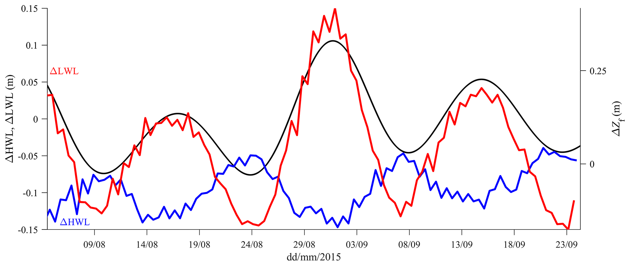
Figure 5Differences in the relative water level between St3 and St0, showing the fortnightly tide (ΔZf; black line; right axis), ΔHWL (blue line; left axis), and ΔLWL (red line; left axis).
4.2 Neap and spring waves propagation
The observed tidal waves on 24 (neap) and 31 (spring) August at stations 0 to 6 are illustrated in Fig. 6. On both dates, the wave is sinusoidal near the mouth (St0); as it propagates upstream, the wave remains approximately sinusoidal at neap tide but is increasingly distorted at spring tide (the ebb and flood phases become typically longer and shorter, respectively).
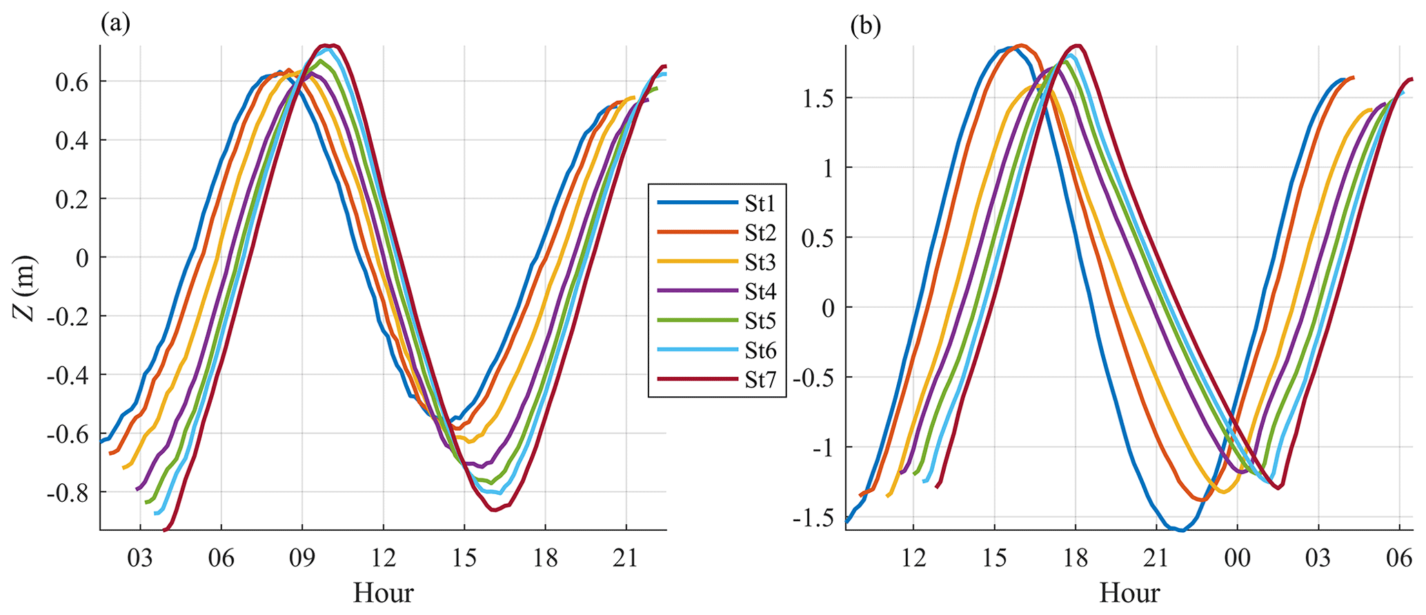
Figure 6Water level variations (Z; metres) at stations St0–6 for (a) neap (24 August 2015) and (b) spring (31 August 2015) tides.
The diurnal (D1), semi-diurnal (D2), and quarter-diurnal (D4) species contained in the tidal signal were extracted with a wavelet analysis of the non-filtered pressure records (Fig. 7). Note that the sixth-diurnal species were not analysed since their magnitudes are relatively small when compared with other components (see Garel and Cai, 2018). The amplitude of D1 is relatively low and constant along the channel on both neap and spring tides (Fig. 7a). D2 is responsible for most of the tidal wave height variations along the channel (Fig. 7b), due to the predominance of the M2 constituent. On spring (neap) tide, D2 is damped (amplified) along the lower estuary half, while it is similarly amplified on both spring and neap tides along the upper half. These along-channel variations in tidal elevation are noticeable in Fig. 6. The amplitude of D4 also features significant differences between spring and neap tides (Fig. 7c), i.e. it is weak (<3 cm) and nearly constant for the neap tide, while it grows upstream for the spring tide from 4 cm at St0 up to approximately 20 cm at St6. The quarter-diurnal species consists mainly of M4 (interaction of M2 with itself) and MS4 (M2–S2 interaction), both of equivalent importance in the Guadiana Estuary (Garel and Cai, 2018). Typically, the growth of these constituents in the upstream direction indicates increasing distortion of the tidal wave due to the combined effects from the nonlinear continuity term, convective acceleration term, and quadratic friction in both mass and momentum equations (Parker, 1991). Such along-channel wave distortion is apparent at spring tide in Fig. 6b.
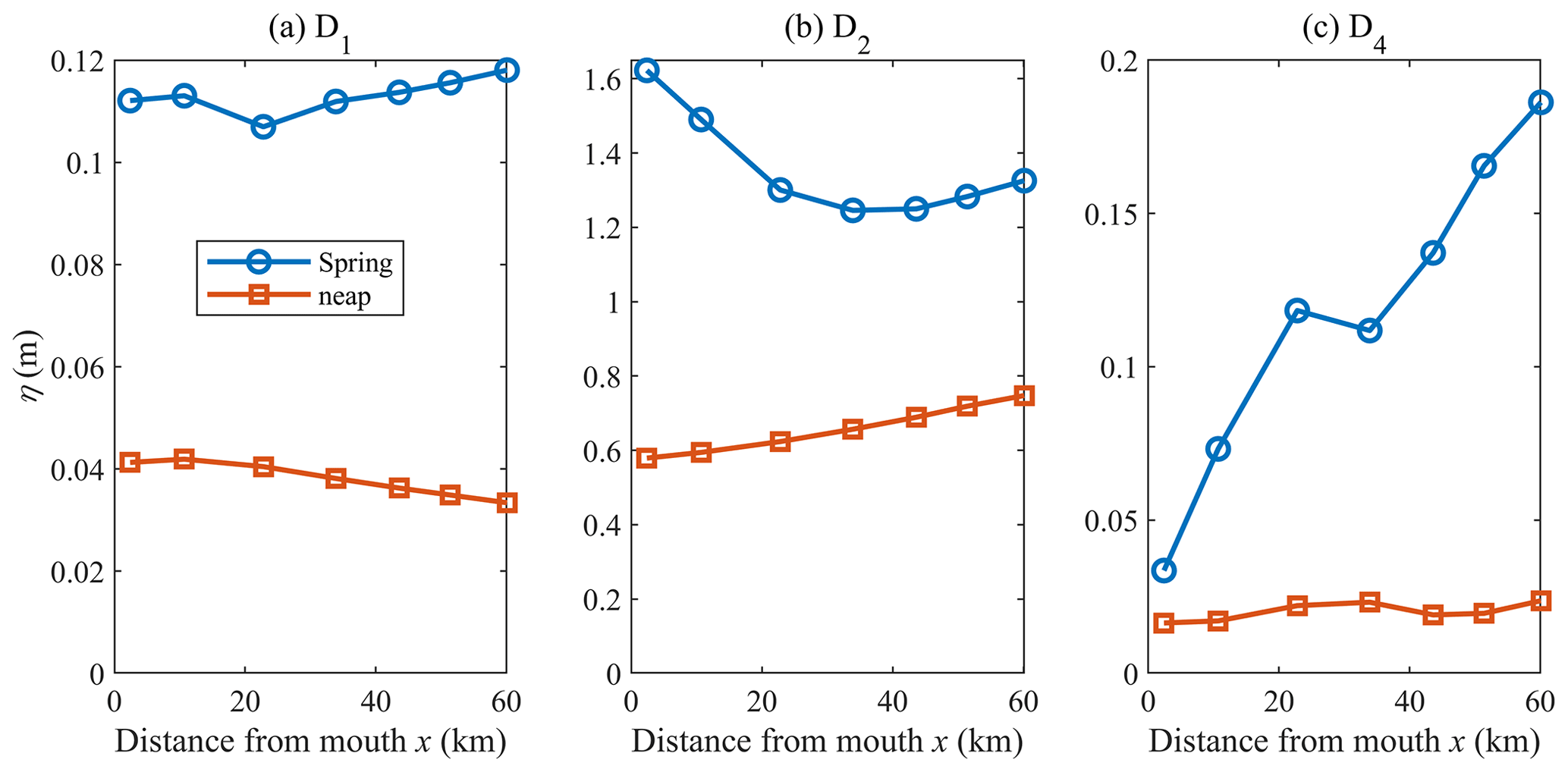
Figure 7Amplitude (η; metres) of the (a) diurnal D1 (b) semi-diurnal D2, and (c) quarter-diurnal D4 tidal species along the channel during the largest spring (blue line; 31 August 2015) and lowest neap (red line; 24 August 2015) tides.
Amongst the three main tidal species at the Guadiana Estuary, D2 is characterized by damping patterns that account for the previously reported fortnightly Zf modulations resulting from temporal LWL slope variations along the lower reach. There, the opposite semi-diurnal wave patterns on neap (amplification) and spring (damping) tides are due to variations in friction; frictional effects dominate morphological convergence effects on spring tide, and the opposite occurs on neap tide (Garel and Cai, 2018). In contrast, along the upper reach, where the fortnightly wave height is constant, D2 amplifies similarly on springs and neaps due to reflection at the head that reduces the overall friction experienced by the (spring) wave (Garel and Cai, 2018). These observations indicate that the fortnightly tide amplitude along the channel is intrinsically linked, through friction, to the neap–spring variability in the damping patterns of the semi-diurnal wave propagating upstream. In the next section, the fortnightly tide hydrodynamics are further explored with an analytical model considering a M2 wave with variable amplitude.
5.1 Model implementation
The hydrodynamic model of tidal propagation described in Sect. 3.2 was implemented at the Guadiana Estuary in order to compute the residual slope using Eq. (4). The model was set up with the same parameters as those in Garel and Cai (2018), considering a flat bed and semi-closed channel, with a cross-sectional area convergence length (a) of 31 km and width convergence length (b) of 38 km (Eqs. 6 and 7), that accurately represents the estuary geometry. The model was calibrated with a Manning–Strickler coefficient K of 47 m s−1. Considering a flat, non-rippled, sandy bed, K is related to the drag coefficient (Cd) through the following (Soulsby, 1997):
A typical value for the bed roughness in estuaries is Z0= 0.7 mm, corresponding to mixed (non-rippled) sand and mud surface sediment. Thus, for the mean water depth of 5.5 m considered here, the drag coefficient from Eq. (9) is . This coefficient is in the range of typical values applicable to depth-averaged currents in estuaries, typically of the order of – (Dronkers, 2005; see also Li et al., 2004). This value yields a Manning–Strickler coefficient K=47 m s−1, which matches the value used to calibrate the model. The calibrated model reproduces the observed properties (amplitude and phase) of the spring and neap semi-diurnal tides along the channel remarkably well when considering a M2 wave of variable amplitude (see Garel and Cai, 2018).
To facilitate comparisons with observations, the mean value of the tidal average () time series predicted by Eq. (4) was removed in order to obtain MWL variations around zero (denoted as Zm, hereafter) at each position along the channel (as for Zf at St0–6). Furthermore, the observed Zf at each station was corrected from the value at St0 to obtain Zf= 0 at the mouth (as for Zm). Finally, the records at St1 were substituted by interpolated values between St0 and St2 to discard the incongruous observations reported in Sect. 4.1.
The model reproduces the observed fortnightly tide remarkably well (Fig. 8). Zm increases asymptotically along the lower estuary half only, with the largest amplitude (about 10–15 cm) on the largest spring tides. The tendency for the observed Zf to be slightly higher (on springs) and lower (on neaps) than Zm at St6 is attributed to backwater effects induced by a sill across the channel near the estuary head, which is not included in the model (see Garel and Cai, 2018). Overall, the correspondence of the analytical results with observations confirms that the fortnightly tide at the Guadiana Estuary results from intratidal variations in friction produced by distinct tidal stages.
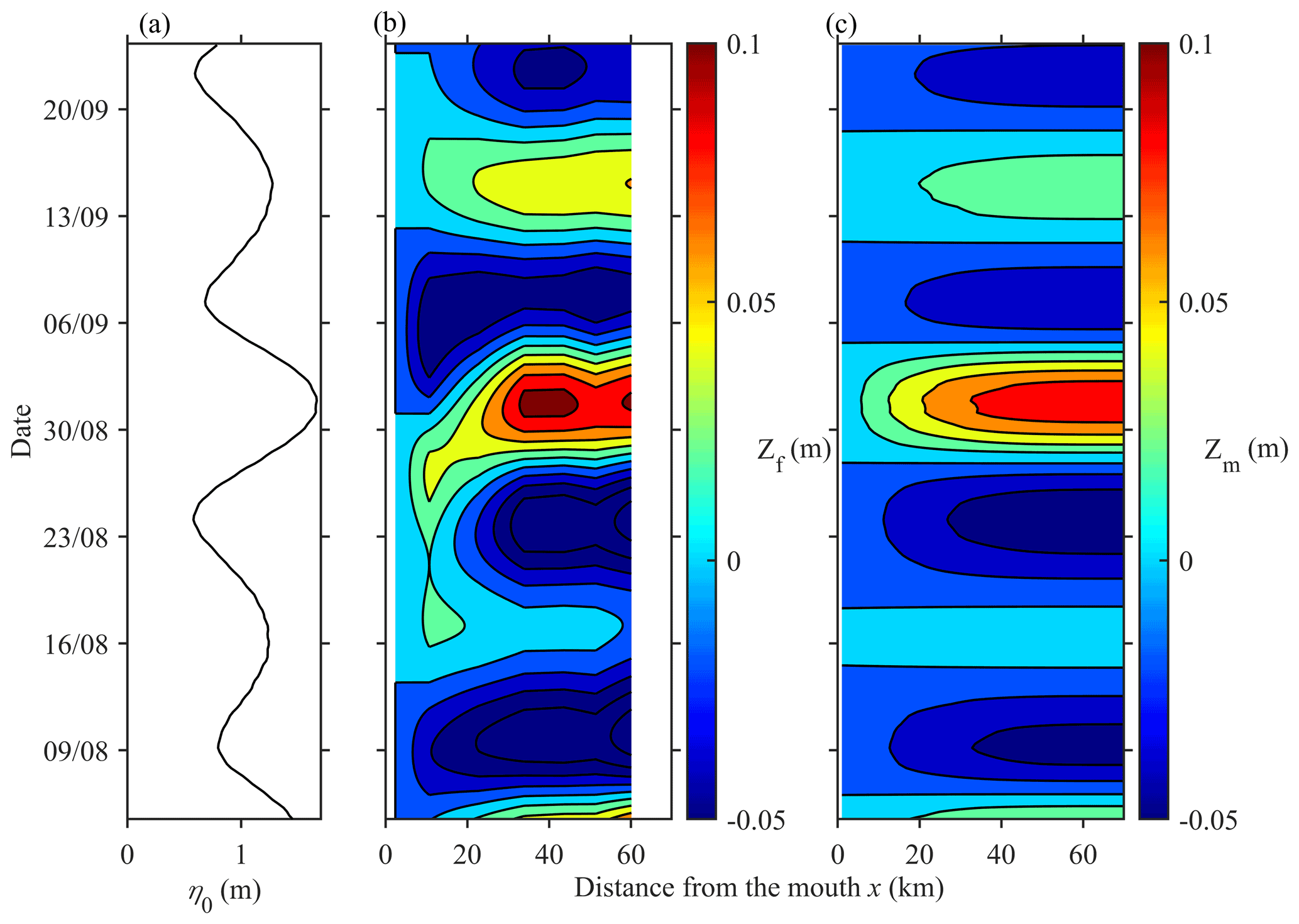
Figure 8(a) Tidal amplitude at the mouth (η0; metres). (b) Observed (Zf) and (c) simulated (Zm) fortnightly water level variations along the Guadiana Estuary.
5.2 Fortnightly tide dynamics
This section examines the relations between the fortnightly tide development and the main dimensional parameters that describe the M2 tide propagation (Table 1), including the damping number for water level, δA (i.e. the rate of increase, δA >0, or decrease, δA <0, of the wave amplitude along the estuary), the friction number χ (which represents the contribution of frictional dissipation), the celerity number for water level, λA (i.e. the wave speed relative to the frictionless wave celerity c0, which is <1 for waves faster than c0), and the phase difference ϕ between velocity and elevation. Both semi-closed and infinite channels (denoted hereafter as SC and IC, respectively) are considered to make explicit the effect of wave reflection at the head. Figure 9 represents the variations in the MWL slope (S), δA, λA, χ, and ϕ along the channel in function of the tidal forcing for both SC (Fig. 9a–e; left column) and IC (Fig. 9k–o; right column). To highlight the fortnightly variability in each parameter, the middle column (Fig. 9f–i) indicates their difference (ΔS, ΔδA, ΔλA, Δχ, and Δϕ), considering the strongest (spring) and weakest (neap) tidal forcings (with SC as solid lines and IC as dashed lines).
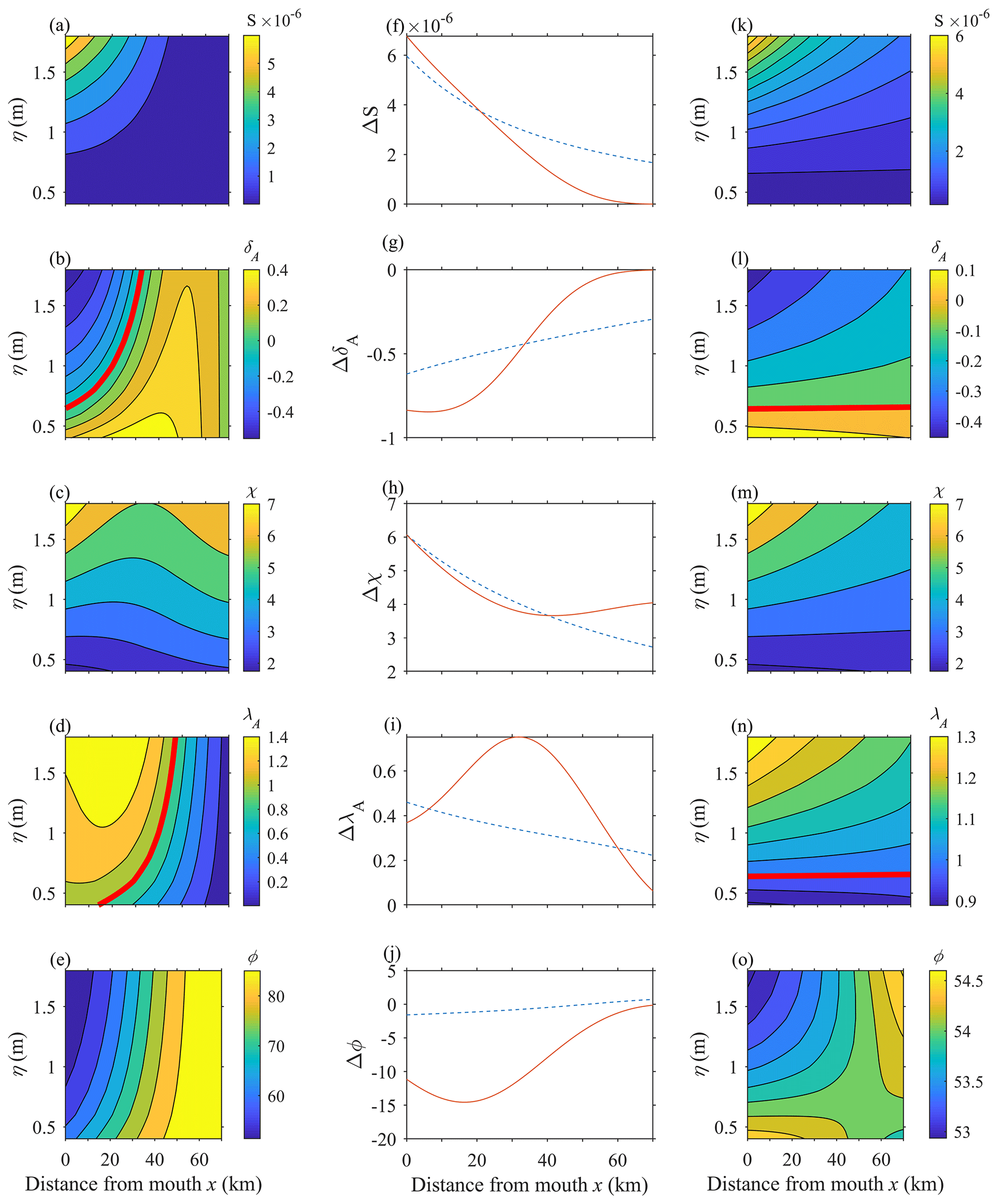
Figure 9Tidally averaged slope (S) and main dimensionless parameters describing the tidal propagation along the Guadiana Estuary in function of the tidal amplitude at the mouth (η0; metres). The damping number for the water level (δA), the friction number (χ), the celerity number for water level (λA), and the phase angle between velocity and elevation (ϕ) are shown. The left column (a–e) and the right column (k–o) represent the results for a semi-closed channel and an infinite channel, respectively. The middle column (f–j) represents the spring-neap difference for each parameter (ΔS, ΔδA, ΔλA, and Δϕ, respectively). The thick red lines presented in subplots (b) and (l) correspond to δA=0. In subplots (d) and (n), they correspond to λA=1.
The slope S increases with tidal forcing along the lower half of the SC channel but becomes insignificant upstream (Fig. 9a). Thus, the spring–neap difference in slope (ΔS) becomes negligible at mid-estuary (Fig. 9f), and the fortnightly tide amplitude grows along the lower reach, as previously observed (Figs. 2a and 8a). In contrast, a significant slope S develops along the entire infinite channel for tidal amplitudes larger than the mean value of 1 m, approximately (Fig. 9k). In this case, the fortnightly tide amplitude grows from the mouth to the head (see ΔS in Fig. 9f; dashed line). Such a pattern has been typically observed in many long estuaries, although they are subject to substantial river discharge, where the MSf propagates much further landward that the semi-diurnal and diurnal tidal constituents (e.g. Buschman et al., 2009; Gallo and Vinzon, 2005; Godin, 1999; Godin and Martínez, 1994; Matte et al., 2014). In these settings, the river discharge effect can be accounted for by enhanced friction, increasing the tidal asymmetry in discharge and, hence, the fortnightly tide amplitude (Godin, 1985, 1999; Laurel-Castillo and Valle-Levinson, 2020; Sassi and Hoitink, 2013; Savenije and Veling, 2005). Fortnightly oscillations of the MWL eventually exceed the amplitude of the main tidal constituents, with mean LWL progressively being lowered during neap tides rather than spring tides (Gallo and Vinzon, 2005; LeBlond, 1979, 1991). Moreover, general observations of long systems indicate that the MSf amplitude maxima are located further landward than the maxima in the overtides (Gallo and Vinzon, 2005; Guo et al., 2015; Jay et al., 2015), which is not the case at the Guadiana Estuary (compare Figs. 3b and 7c). Overall, the analytical results show that wave reflection at the head inhibits the growth of the fortnightly tide along the upper reach of estuaries.
Figure 9b and l illustrate how reflection affects the semi-diurnal wave amplitude variations along the channel. The wave shoals along the SC channel for tidal amplitude <0.7 m (Fig. 9b). For larger tidal forcing, the wave is increasingly damped along the lower half of the channel but remains amplified upstream. Near the head, the wave shoals independently of the tidal forcing (as indicated by the verticalized isocontours in Fig. 9b). The spring–neap difference in damping ΔδA is insignificant along the upper estuary half (Fig. 9g; solid line), indicating that the difference in amplitude between the neap and spring waves remains constant (the wave is amplified in both cases). For an IC channel, the M2 wave is damped along the entire system for tidal forcing >0.6 m and amplified otherwise (Fig. 9l). Yet, damping is relatively weak, as indicated by the sub-horizontal contours on Fig. 9l. Thus, ΔδA remains significant from the mouth to the head (Fig. 9g; dashed line).
Due to its nonlinear depth dependence, the friction number (χ) reflects the above-described variations in the M2 wave height. In particular, χ increases (decreases) with the tidal forcing or for shoaling (damped) waves (Fig. 9c, m). The frictional dissipation in the lower half of the estuary is similar for the SC and IF channels, indicating similar M2 amplitude in both cases (Fig. 9b, l). In contrast, at the upper channel half, friction increases for SC and decreases for IF, in particular for large tidal forcing, due to opposite shoaling patterns. Hence, the greatest spring–neap differences in the friction term (Δχ) between the SC and IF channels are in the upper 30 km (Fig. 9h). This pattern indicates a significantly higher spring wave for SC than IF along this reach. Overall, the main effect of wave reflection at the head is to amplify the M2 wave along the upper channel half, in particular for large tidal forcing. Compared to the IF case, these dynamics should enhance the MWL slope at springs and, thus, the MSf amplitude at the upper reach, which is opposed to the observations (see Fig. 2).
It can also be observed that, for both the SC and IF channels, the M2 wave accelerates with decreasing tidal forcing (Fig. 9d, n). Thus, the wave travels faster on a neap tide than on a spring tide. This pattern is explained by tidal damping effects on progressive waves' celerity (Savenije et al., 2008; Savenije and Veling, 2005). As observed in many estuaries (e.g. the Thames, Sheldt, and Incomati), damped waves propagate slower than the classical wave celerity c0 (corresponding to the frictionless case), while amplified waves often travel significantly faster than c0. This phenomenon occurs because changes in the height of a propagating wave affect the phase difference ϕ between the horizontal and vertical tides (which is otherwise constant in the frictionless case). For IF channels, where damping is weak, the phase is relatively constant both spatially and temporally (between 53 and 54.5∘; Fig. 9o). The difference in phase between spring and neap tides (Δϕ) is < 2∘ (Fig. 9j; dashed line), indicating that the ebb–flood discharge asymmetry remains constant along the entire channel. As the wave height is only slightly damped, this asymmetry produces a significant MWL slope along the entire channel at spring tide. For the SC channel, the phase lead varies significantly as the wave propagates upstream (see the vertical contours in Fig. 9e). This is because the tidal wave tends to show a standing behaviour (ϕ≃ 90∘) towards the head. The difference in phase between neap and spring tides, Δϕ, is maximum at the lower reach (up to 15∘, representing a difference of about 31 min for a M2 tide) but has a weak incidence on the fortnightly slope which is slightly larger than for IF at this location (Fig. 9f). The main effect of reflection is in the upper reach where HWL and LWL occur close to slack water, reducing the tidal discharge asymmetry. Hence, the discharge asymmetry is not sufficient to produce a significant MWL slope on springs in the upper estuary half, although the wave is larger than for the IF channel.
5.3 Fortnightly tide amplitude and potential implications on estuarine environment
In this section, the analytical model is exploited to analyse the fortnightly variations in MWL for SC channels with distinct geometry (depth, length, and morphological convergence). Implications for water resources management in semi-arid systems are also discussed.
First, the maximum MWL () is predicted in function of the tidal forcing, using the analytical model that was set up for the Guadiana Estuary (see Sect. 5.1). Overall, the tidal forcing largely controls , which is significant (e.g. >0.5 m) for macrotidal (η> 2 m), shallow, weakly convergent, and long systems (Fig. 10a–c, respectively). Of the three geometric parameters considered, the mean depth has the strongest influence on (Fig. 10a), as expressed in Eq. (4). The two other parameters affect the most in the case of strongly convergent and short channels (as indicated by the sub-vertical contours in Fig. 10b, c), but the maximum MWL tends to remain small. For short systems, the superimposition of the incident and reflected wave typically produces a standing wave (Cai et al., 2016b). In strongly convergent systems, the tide propagates as an apparent standing wave (Friedrichs and Aubrey, 1994; Hunt, 1964; Jay, 1991; Savenije et al., 2008; van Rijn, 2011). In both cases, the tidal discharge asymmetry is negligible (the phase difference between velocity and elevation is close to 90∘), inhibiting the growth of along the channel.
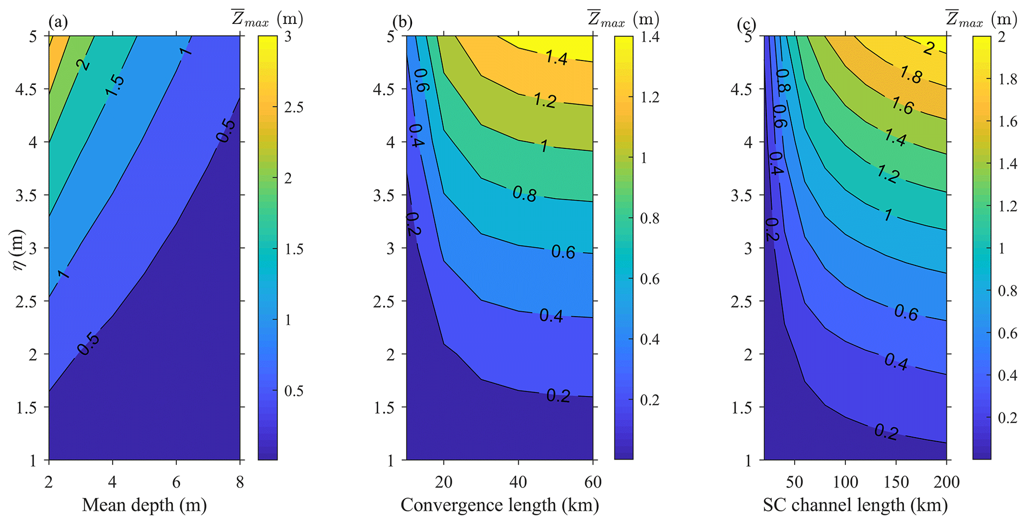
Figure 10Maximum tidally averaged water level () as a function of the tidal forcing and mean depth (a), convergence length (b), and estuary length (c) at a semi-closed channel.
Second, the position of along the channel is investigated for SC channels with usual geometric settings (i.e. estuary length of 20–200 km, convergence length of 20–100 km, and mean depth of 2–8 m). This position is defined at the distance from the mouth where the slope becomes negligible (<0.1 cm km−1) and is denoted Xs=0. Results are reported in Fig. 11, considering a tidal amplitude of 2 m at the mouth. A total of two geometric parameters are evaluated, while the value of the third parameter corresponds to the one at the Guadiana Estuary (i.e. the convergence length is 38 km, the estuary length is 78 km, and the water depth is 5.5 m in Fig. 11a, b, and c, respectively). In general, the slope becomes negligible slightly upstream of the mid-estuary length. This position varies weakly upstream or downstream with the convergence length and mean depth, except for deep and highly convergent systems where Xs=0 is close to the mouth (Fig. 11b). In all the evaluated cases, the slope is flat along the upper estuary reach, contrary to infinite channels where is located at the estuary head.
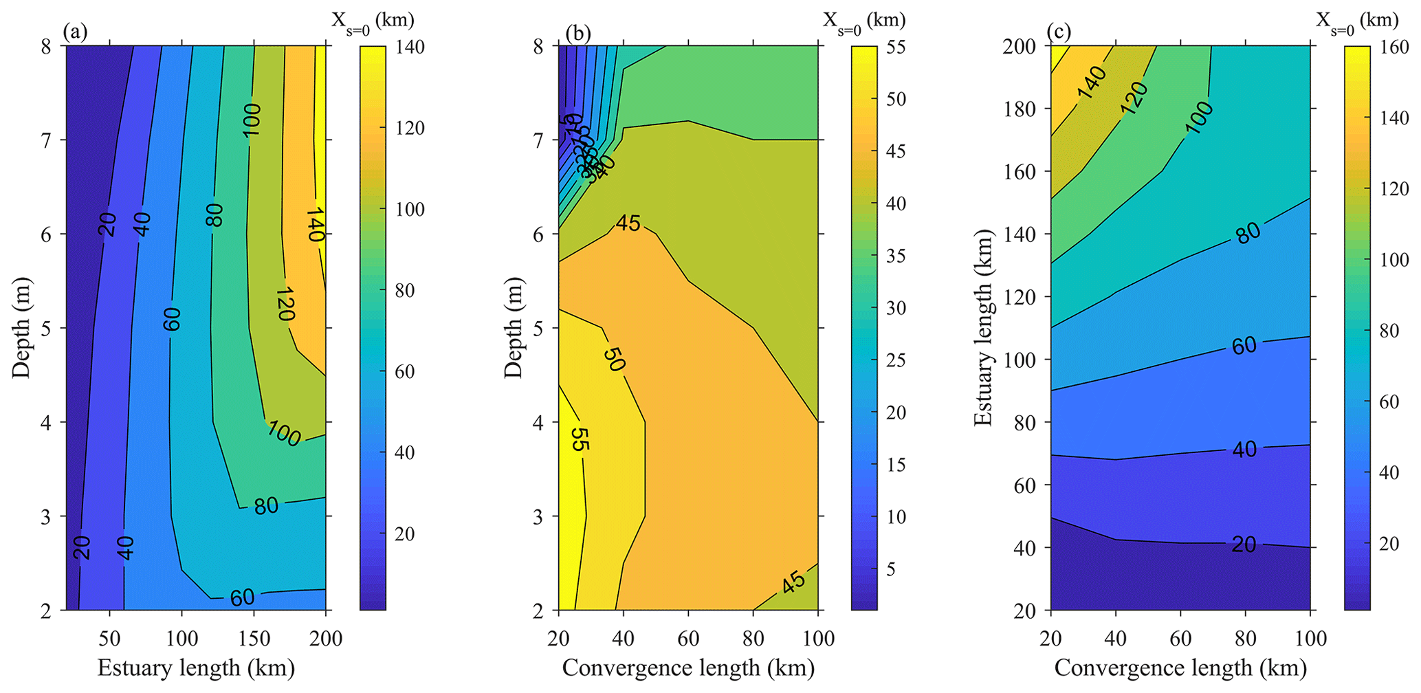
Figure 11Position of the negligible slope (XS=0; in kilometres) along a semi-closed channel with distinct geometric settings. In panel (a), the convergence length is 38 km. In panel (b), the estuary length is 78 km. In panel (c), the water depth is 5.5 m.
The above results indicate that morphological changes in tidally dominated estuaries with negligible river discharge affect fortnightly water level variations along the channel. In particular, both an increased mean depth (due to channel dredging or to sea level rise) and the installation of a tidal barrage (reducing the channel length) decrease the maximum fortnightly tide amplitude along the estuary (Fig. 10a, c). A greater depth reduces the friction of the propagating semi-diurnal tidal wave and, hence, the MWL slope. Enhanced reflection effects by tidal barrages restrict the MWL growth to the first half of the (shorter) estuary, especially during spring tides. For both cases, the reduced growth of MSf amplitude implies weaker spring–neap differences in the LWL along the channel (e.g. Fig. 5). Margins usually exposed to air on spring low tide may experience permanent inundation in the modified estuary. Such changes in the tidal inundation regime can have severe impacts on estuarine environments. In particular, tidal inundation is a fundamental driver of wetland functions, and even small changes can influence the extent and function of salt marsh habitats (Janousek and Folger, 2014; Valiela et al., 1978). An increased LWL also enhances flooded areas during strong river discharge events, which are predicted to increase both in intensity and frequency in semi-arid regions (e.g. Smith, 1996; Tabari, 2020). Moreover, in comparison with (diurnal and semi-diurnal) tidal components that dominate at the mouth, the upstream mass transport by MSf motions is more effective due to a longer wavelength (Buijsman and Ridderinkhof, 2007; MacMahan et al., 2014). In particular, variations in subtidal water level are directly linked to salt intrusion into estuaries (Henrie and Valle-Levinson, 2014). Reductions in the fortnightly tide amplitude in modified estuaries may, therefore, have significant effects on water quality and ecology. These potential effects on the fortnightly tide are particularly relevant for macrotidal semi-arid estuaries like those found in NE Brazil (e.g. Barletta and Costa, 2009; Clark and Pessanha, 2014; Dias et al., 2009; Frazão and Vital, 2006).
Using analytical solutions, this study has examined the fortnightly water level variations due to tidal motions alone in tide-dominated estuaries with negligible river discharge. These systems are typically found in semi-arid regions, where the river discharge is negligible during a large part of the year. In the Guadiana Estuary, pressure measurements in August–September 2015 show that the MWL along the estuary is typically higher on spring tide and lower on neap tide. These fluctuations result from an increase in the relative LWL in the upstream direction on spring tides, while the relative HWL remains approximatively constant. The MSf amplitude grows from the mouth until the mid-estuary and remains constant upstream. During the survey, weather conditions were fair, and the fortnightly tide represented about half of the subtidal signal in the upper estuary half. The other main contribution, with approximately constant amplitude from the mouth to the head, was induced by wind (not studied further in the present paper). The contribution of neap–spring differences in water density is negligible.
It is confirmed that the fortnightly tide is produced by intratidal variations in friction using an analytical model of wave propagation. Frictional asymmetries relate mainly to the nonlinear depth dependence of friction to water depth which strongly (weakly) affects the balance between ebb and flood discharges on springs (neaps). Considering a semi-closed channel, the model results match the observations, indicating that the MSf growth in the first half of the estuary is due to reflection effects at the head. Reflection affects MWL mainly through modification of the phase difference between velocity and elevation, which increases in the upstream direction (the wave is standing near the head due to the superimposition of the incident and reflected waves). The low and high water levels come progressively closer to slack water, reducing the flood–ebb discharge asymmetry. In the upper half of the estuary, the discharge asymmetry becomes negligible, despite wave shoaling. Overall, observations of a flat MWL along a significant portion of the upper estuary, particularly on springs, may indicate the presence of significant reflection effects. These data are generally easier to obtain than the phase difference, which requires combined velocity and elevation records.
Finally, changes in the mean depth (e.g. due to dredging or sea level rise) or in the channel length (e.g. due to the installation of a tidal barrage) affect the MSf amplitudes along semi-arid estuaries with negligible river discharge. Impacts on the ecosystem may arise from the induced modification of the inundation regime (through changes of the MWL and LWL) and of the upstream mass transport, in particular in macrotidal regions.
The data and source codes used to reproduce the experiments presented in this paper are available from the authors upon request (egarel@ualg.pt).
All authors contributed to the design and development of this work. The experiments were originally carried out by HC. PZ carried out the data analysis. EG built the model and wrote the paper.
The contact author has declared that neither they nor their co-authors have any competing interests
Publisher’s note: Copernicus Publications remains neutral with regard to jurisdictional claims in published maps and institutional affiliations.
The authors would like to thank Marco Toffolon, from Trento University, who raised the issue of fortnightly water level dynamics in tide-dominated estuaries.
This research has been supported by the Portuguese Foundation for Science and Technology (FCT; grant no. UID/MAR/00350/2020) and the National Natural Science Foundation of China (grant no. 51979296).
This paper was edited by Neil Wells and reviewed by two anonymous referees.
Aubrey, D. G. and Speer, P. E.: A study of non-linear tidal propagation in shallow inlet/estuarine systems Part I: Observations, Estuar. Coast. Shelf S., 21, 185–205, https://doi.org/10.1016/0272-7714(85)90097-6, 1985.
Barletta, M. and Costa, M. F.: Living and non-living resources exploitation in a tropical semi-arid estuary, J. Coastal Res., SI 56, 371–375, https://www.jstor.org/stable/25737600, last access: 1 November 2021, 2009.
Buijsman, M. C. and Ridderinkhof, H.: Long-term ferry-ADCP observations of tidal currents in the Marsdiep inlet, J. Sea Res., 57, 237–256, https://doi.org/10.1016/j.seares.2006.11.004, 2007.
Buschman, F. A., Hoitink, A. J. F., van der Vegt, M., and Hoekstra, P.: Subtidal water level variation controlled by river flow and tides, Water Resour. Res., 45, W10420, https://doi.org/10.1029/2009WR008167, 2009.
Cai, H., Savenije, H. H. G., and Toffolon, M.: Linking the river to the estuary: influence of river discharge on tidal damping, Hydrol. Earth Syst. Sci., 18, 287–304, https://doi.org/10.5194/hess-18-287-2014, 2014.
Cai, H., Savenije, H. H. G., Jiang, C., Zhao, L., and Yang, Q.: Analytical approach for determining the mean water level profile in an estuary with substantial fresh water discharge, Hydrol. Earth Syst. Sci., 20, 1177–1195, https://doi.org/10.5194/hess-20-1177-2016, 2016a.
Cai, H., Toffolon, M., and Savenije, H. H. G.: An analytical approach to determining resonance in semi-closed convergent tidal channels, Coast Eng. J., 58, 1650009, https://doi.org/10.1142/S0578563416500091, 2016b.
Cai, H., Savenije, H. H. G., Garel, E., Zhang, X., Guo, L., Zhang, M., Liu, F., and Yang, Q.: Seasonal behaviour of tidal damping and residual water level slope in the Yangtze River estuary: identifying the critical position and river discharge for maximum tidal damping, Hydrol. Earth Syst. Sci., 23, 2779–2794, https://doi.org/10.5194/hess-23-2779-2019, 2019.
Clark, F. J. K., and Pessanha, A. L. M.: Diet and ontogenetic shift in habitat use by Rhinosardinia bahiensis in a tropical semi-arid estuary, north-eastern Brazil, J. Mar. Biol. Assoc. UK, 95, 175–183, https://doi.org/10.1017/S0025315414000939, 2014.
Correia, C., Torres, A. F., Rosa, A., Cravo, A., Jacob, J., de Oliveira Júnior, L., and Garel, E.: Export of dissolved and suspended matter from the main estuaries in South Portugal during winter conditions, Mar. Chem., 224, 103827, https://doi.org/10.1016/j.marchem.2020.103827, 2020.
Descroix, L., Sané, Y., Thior, M., Manga, S.-P., Ba, B. D., Mingou, J., Mendy, V., Coly, S., Dièye, A., Badiane, A., Senghor, M.-J., Diedhiou, A.-B., Sow, D., Bouaita, Y., Soumaré, S., Diop, A., Faty, B., Sow, B. A., Machu, E., Montoroi, J.-P., Andrieu, J., and Vandervaere, J.-P.: Inverse Estuaries in West Africa: Evidence of the Rainfall Recovery?, Water, 12, 647, https://doi.org/10.3390/w12030647, 2020.
Dias, F. J. S., Marins, R. V., and Maia, L. P.: Hydrology of a well-mixed estuary at the semi-arid Northeastern Brazilian coast, Acta Limnologica Brasiliensia, 21, 377–385, 2009.
Dias, F. J. d. S., Castro, B. M., Lacerda, L. D., Miranda, L. B., and Marins, R. V.: Physical characteristics and discharges of suspended particulate matter at the continent-ocean interface in an estuary located in a semiarid region in northeastern Brazil, Estuar. Coast. Shelf S., 180, 258–274, https://doi.org/10.1016/j.ecss.2016.08.006, 2016.
Dronkers, J.: Dynamics of Coastal Systems, World Scientific, World Scientific Publishing Co. Pte. Ltd, Singapore, 780 pp., ISBN: 9787521002966, https://doi.org/10.1142/5781, 2005.
Dworak, J. A. and Gomez-Valdes, J.: Modulation of shallow water tides in an inlet-basin system with a mixed tidal regime, J. Geophys. Res.-Oceans, 110, C01007, https://doi.org/10.1029/2003JC001865, 2005.
Feng, S. and Fu, Q.: Expansion of global drylands under a warming climate, Atmos. Chem. Phys., 13, 10081–10094, https://doi.org/10.5194/acp-13-10081-2013, 2013.
Frazão, E. P. and Vital, H.: Hydrodynamic and Morpho-Sedimentary Characterization of the Potengi Estuary and Adjacent Areas (NE Brazil): Subsidies Towards Oil Spilling Environmental Control, J. Coastal Res., SI 39, 1446–1449, https://www.jstor.org/stable/25742994, last access: 1 November 2021, 2006.
Friedrichs, C. T. and Aubrey, D. G.: Non-linear tidal distortion in shallow well-mixed estuaries: a synthesis, Estuar. Coast. Shelf S., 27, 521–545, https://doi.org/10.1016/0272-7714(88)90082-0, 1988.
Friedrichs, C. T. and Aubrey, D. G.: Tidal propagation in strongly convergent channels, J. Geophys. Res.-Oceans, 99, 3321–3336, https://doi.org/10.1029/93JC03219, 1994.
Frota, F. F., Paiva, B. P., and Schettini, C. A. F.: Intra-tidal variation of stratification in a semi-arid estuary under the impact of flow regulation, Braz. J. Oceanogr., 61, 23–33, https://doi.org/10.1029/96jc00630, 2013.
Gallo, M. N. and Vinzon, S. B.: Generation of overtides and compound tides in Amazon estuary, Ocean Dynam., 55, 441–448, https://doi.org/10.1007/s10236-005-0003-8, 2005.
Garel, E.: Present Dynamics of the Guadiana Estuary, in: Guadiana River estuary – Investigating the past, present and future, edited by: Moura, D., Gomes, A., Mendes, I., and Anílbal, J., University of Algarve, Faro, 15–37 pp., 2017.
Garel, E. and D'Alimonte, D.: Continuous river discharge monitoring with bottom-mounted current profilers at narrow tidal estuaries, Cont. Shelf Res., 133, 1–12, https://doi.org/10.1016/j.csr.2016.12.001, 2017.
Garel, E. and Cai, H.: Effects of Tidal-Forcing Variations on Tidal Properties Along a Narrow Convergent Estuary, Estuar. Coast., 41, 1924–1942, https://doi.org/10.1007/s12237-018-0410-y, 2018.
Garel, E., Pinto, L., Santos, A., and Ferreira, Ó.: Tidal and river discharge forcing upon water and sediment circulation at a rock-bound estuary (Guadiana estuary, Portugal), Estuar. Coast. Shelf S., 84, 269–281, https://doi.org/10.1016/j.ecss.2009.07.002, 2009.
Godin, G.: Modification of River Tides by the Discharge, J. Waterw. Port Coast., 111, 257–274, https://doi.org/10.1016/0198-0254(85)92663-9, 1985.
Godin, G.: The Propagation of Tides up Rivers with Special Considerations on the Upper Saint Lawrence River, Estuar. Coast. Shelf S., 48, 307–324, https://doi.org/10.1006/ecss.1998.0422, 1999.
Godin, G. and Martínez, A.: Numerical experiments to investigate the effects of quadratic friction on the propagation of tides in a channel, Cont. Shelf Res., 14, 723, https://doi.org/10.1016/0278-4343(94)90070-1, 1994.
Guo, L., van der Wegen, M., Jay, D.A., Matte, P., Wang, Z.B., Roelvink, D., and He, Q.: River-tide dynamics: Exploration of nonstationary and nonlinear tidal behavior in the Yangtze River estuary, J. Geophys. Res.-Oceans, 120, 3499–3521, https://doi.org/10.1002/2014JC010491, 2015.
Henrie, K. and Valle-Levinson, A.: Subtidal variability in water levels inside a subtropical estuary, J. Geophys. Res-Oceans, 119, 7483–7492, https://doi.org/10.1002/2014JC009829, 2014.
Hoitink, A. J. F. and Jay, D. A.: Tidal river dynamics: Implications for deltas, Rev. Geophys., 54, 240–272, https://doi.org/10.1002/2015RG000507, 2016.
Hunt, J. N.: Tidal Oscillations in Estuaries, Geophys. J. Royal Astronom. Soc., 8, 440–455, https://doi.org/10.1111/j.1365-246X.1964.tb03863.x, 1964.
Janousek, C. N. and Folger, C. L.: Variation in tidal wetland plant diversity and composition within and among coastal estuaries: assessing the relative importance of environmental gradients, J. Vegetation S., 25, 534–545, https://doi.org/10.1111/jvs.12107, 2014.
Jay, D. A.: Green's law revisited: Tidal long-wave propagation in channels with strong topography, J. Geophys. Res.-Oceans, 96, 20585–20598, https://doi.org/10.1029/91JC01633, 1991.
Jay, D. A. and Flinchem, E. P.: Interaction of fluctuating river flow with a barotropic tide: A demonstration of wavelet tidal analysis methods, J. Geophys. Res.-Oceans, 102, 5705–5720, https://doi.org/10.1029/96JC00496, 1997.
Jay, D. A., Leffler, K., and Degens, S.: Long-Term Evolution of Columbia River Tides, J. Waterw. Port C., 137, 182–191, https://doi.org/10.1061/(ASCE)WW.1943-5460.0000082, 2011.
Jay, D. A., Leffler, K., Diefenderfer, H. L., and Borde, A. B.: Tidal-Fluvial and Estuarine Processes in the Lower Columbia River: I. Along-Channel Water Level Variations, Pacific Ocean to Bonneville Dam, Estuar. Coast., 38, 415–433, https://doi.org/10.1007/s12237-014-9819-0, 2015.
Lamontagne, S., Deegan, B. M., Aldridge, K. T., Brookes, J. D., and Geddes, M. C.: Fish diets in a freshwater-deprived semiarid estuary (The Coorong, Australia) as inferred by stable isotope analysis, Estuar. Coast. Shelf S., 178, 1–11, https://doi.org/10.1016/j.ecss.2016.05.016, 2016.
Laurel-Castillo, J. A. and Valle-Levinson, A.: Tidal and subtidal variations in water level produced by ocean-river interactions in a subtropical estuary, J. Geophys. Res.-Oceans, 125, e2018JC014116, https://doi.org/10.1029/2018JC014116, 2020.
Leblanc, M., Tweed, S., Van Dijk, A., and Timbal, B.: A review of historic and future hydrological changes in the Murray-Darling Basin, Global Planet, Change, 80, 226, https://doi.org/10.1016/j.gloplacha.2011.10.012, 2012.
LeBlond, P. H.: On tidal propagation in shallow rivers, J. Geophys. Res.-Oceans, 83, 4717–4721, https://doi.org/10.1029/JC083iC09p04717, 1978.
LeBlond, P. H.: Forced fortnightly tides in shallow rivers, Atmos. Ocean, 17, 253–264, https://doi.org/10.1080/07055900.1979.9649064, 1979.
LeBlond, P. H.: Tides and their interactions with other oceanographic phenomena in shallow water (review), in: Tidal hydrodynamics, edited by: Parker, B. B., John Wiley and Sons, Hoboken, NJ, 357–378 pp., ISBN: 9780471514985, 1991.
LeBlond, P. H. and Mysak, L. A.: Chapter 8 The Generation and Dissipation of Waves, Elsevier Oceanography, 20, 451–560, https://doi.org/10.1016/S0422-9894(08)70821-3, 1978.
Li, C., Valle-Levinson, A., Atkinson, L. P., Wong, K. C., and Lwiza, K. M. M.: Estimation of drag coefficient in James River Estuary using tidal velocity data from a vessel-towed ADCP, J. Geophys. Res.-Oceans, 109, C03034, https://doi.org/10.1029/2003JC001991, 2004.
Lopez, C. V., Murgulet, D., and Santos, I. R.: Radioactive and stable isotope measurements reveal saline submarine groundwater discharge in a semiarid estuary, J. Hydro., 590, 125395, https://doi.org/10.1016/j.jhydrol.2020.125395, 2020.
MacMahan, J., van de Kreeke, J., Reniers, A., Elgar, S., Raubenheimer, B., Thornton, E., Weltmer, M., Rynne, P., and Brown, J.: Fortnightly tides and subtidal motions in a choked inlet, Estuar. Coast. Shelf S., 150, 325–331, https://doi.org/10.1016/j.ecss.2014.03.025, 2014.
Matte, P., Jay, D. A., and Zaron, E. D.: Adaptation of Classical Tidal Harmonic Analysis to Nonstationary Tides, with Application to River Tides, J. Atmos. Ocean. Tech., 30, 569–589, https://doi.org/10.1175/JTECH-D-12-00016.1, 2013.
Matte, P., Secretan, Y., and Morin, J.: Temporal and spatial variability of tidal-fluvial dynamics in the St. Lawrence fluvial estuary: An application of nonstationary tidal harmonic analysis, J. Geophys. Res.-Oceans, 119, 5724–5744, https://doi.org/10.1002/2014JC009791, 2014.
McCutcheon, M. R., Staryk, C. J., and Hu, X.: Characteristics of the Carbonate System in a Semiarid Estuary that Experiences Summertime Hypoxia, Estuar. Coast., 42, 1509–1523, https://doi.org/10.1007/s12237-019-00588-0, 2019.
Pan, H. and Lv, X.: Reconstruction of spatially continuous water levels in the Columbia River Estuary: The method of Empirical Orthogonal Function revisited, Estuar. Coast. Shelf S., 222, 81–90, https://doi.org/10.1016/j.ecss.2019.04.011, 2019.
Pan, H., Lv, X., Wang, Y., Matte, P., Chen, H., and Jin, G.: Exploration of Tidal-Fluvial Interaction in the Columbia River Estuary Using S_TIDE, J. Geophys. Res-Oceans, 123, 6598–6619, https://doi.org/10.1029/2018JC014146, 2018.
Parker, B. B.: The relative importance of the various nonlinear mechanisms in a wide range of tidal interactions, in: Tidal Hydrodynamics, 237–268, edited by: Parker, B. B., John Wiley and Sons, Hoboken, NJ, ISBN: 9780471514985, 1991.
Prandle, D.: The influence of bed friction and vertical eddy viscosity on tidal propagation, Cont. Shelf Res., 17, 1367–1374, https://doi.org/10.1016/S0278-4343(97)00013-7, 1997.
Ross, L. and Sottolichio, A.: Subtidal variability of sea level in a macrotidal and convergent estuary, Cont. Shelf Res., 131, 28–41, https://doi.org/10.1016/j.csr.2016.11.005, 2016.
Sassi, M. G. and Hoitink, A. J. F.: River flow controls on tides and tide-mean water level profiles in a tidal freshwater river, J. Geophys. Res.-Oceans, 118, 4139–4151, https://doi.org/10.1002/jgrc.20297, 2013.
Savenije, H. H. G.: Salinity and Tides in Alluvial Estuaries, completely revised 2nd edition, http://www.salinityandtides.com (Last access: 1 October, 2021), 2012.
Savenije, H. H. G. and Veling, E. J. M.: Relation between tidal damping and wave celerity in estuaries, J. Geophys. Res.-Oceans, 110, C04007, https://doi.org/10.1029/2004JC002278, 2005.
Savenije, H. H. G., Toffolon, M., Haas, J., and Veling, E. J. M.: Analytical description of tidal dynamics in convergent estuaries, J. Geophys. Res.-Oceans, 113, C10025, https://doi.org/10.1029/2007JC004408, 2008.
Shetye, S. R. and Vijith, V.: Sub-tidal water-level oscillations in the Mandovi estuary, west coast of India, Estuar. Coast. Shelf S., 134, 1–10, https://doi.org/10.1016/j.csr.2016.11.005, 2013.
Smith, J. B.: Standardized estimates of climate change damages for the United States, Climatic Change, 32, 313–326, https://doi.org/10.1007/BF00142467, 1996.
Soulsby, R. L.: Dynamics of Marine Sands, Thomas Telford Publication, London, ISBN: 9780727752314, 249, 1–272 pp., 1997.
Speer, P. E. and Aubrey, D. G.: A study of non-linear tidal propagation in shallow inlet/estuarine systems Part II: Theory, Estuar. Coast. Shelf S., 21, 207–224, https://doi.org/10.1016/0272-7714(85)90097-6, 1985.
Tabari, H.: Climate change impact on flood and extreme precipitation increases with water availability, Sci. Rep-UK, 10, 13768, https://doi.org/10.1038/s41598-020-70816-2, 2020.
Toffolon, M. and Savenije, H. H. G.: Revisiting linearized one-dimensional tidal propagation, J. Geophys. Res.-Oceans, 116, C07007, https://doi.org/10.1029/2010JC006616, 2011.
Valiela, I., Teal, J. M., Volkmann, S., Shafer, D., and Carpenter, E. J.: Nutrient and particulate fluxes in a salt marsh ecosystem: Tidal exchanges and inputs by precipitation and groundwater 1, Limnol. Oceanogr., 23, 798–812, https://doi.org/10.4319/lo.1978.23.4.0798, 1978.
Valle-Levinson, A. and Schettini, C. A. F.: Fortnightly switching of residual flow drivers in a tropical semiarid estuary, Estuar. Coast. Shelf S., 169, 46–55, https://doi.org/10.1016/j.ecss.2015.12.008, 2016.
van Rijn, L. C.: Analytical and numerical analysis of tides and salinities in estuaries; part I: tidal wave propagation in convergent estuaries, Ocean Dynam., 61, 1719–1741, https://doi.org/10.1007/s10236-011-0454-z, 2011.
Vignoli, G., Toffolon, M., and Tubino, M.: Non-linear frictional residual effects on tide propagation, in: Proceedings of XXX IAHR Congress, vol. A, 24–29 August 2003, 291–298, Thessaloniki, Greece, 2003.
Wang, Z., Winterwerp, J., and He, Q.: Interaction between suspended sediment and tidal amplification in the Guadalquivir Estuary, Ocean Dynam., 64, 1487–1498, https://doi.org/10.1007/s10236-014-0758-x, 2014.
Winterwerp, J. C. and Wang, Z. B.: Man-induced regime shifts in small estuaries – I: theory, Ocean Dynam., 63, 1279–1292, https://doi.org/10.1007/s10236-013-0662-9, 2013.
Wong, K. C., Dzwonkowski, B., and Ullman, W. J.: Temporal and spatial variability of sea level and volume flux in the Murderkill Estuary, Estuar. Coast. Shelf S., 84, 440–446, https://doi.org/10.1016/j.ecss.2009.07.008, 2009.