the Creative Commons Attribution 4.0 License.
the Creative Commons Attribution 4.0 License.
 | 08 Nov 2021
Background stratification impacts on internal tide generation and abyssal propagation in the western equatorial Atlantic and the Bay of Biscay
Simon Barbot
Florent Lyard
Michel Tchilibou
Loren Carrere
The forthcoming SWOT altimetric missions aim to resolve the mesoscale with an unprecedented spatial resolution and swath. However, high-frequency processes, such as tides, are undersampled in time and aliased onto lower frequencies, so they need to be corrected properly. Unlike barotropic tides, internal tides (ITs) are not completely stationary and have significant temporal variability due to their interactions with the ocean circulation and the stratification variability. Stratification changes impact both the generation and the propagation of ITs. The present study proposes a methodology to quantify the impacts of background stratification using a clustering method for the classification of a broad range of stratification and idealized modeling of ITs in the frequency domain.
The methodology is successfully tested in the western equatorial Atlantic and in the Bay of Biscay. For the western equatorial Atlantic, a single pycnocline is observed and only the two first vertical modes of ITs have significant amplitudes. With no variation in the stratification intensity, the variation in the depth of this single pycnocline linearly impacts the elevation amplitude, energy fluxes and surface wavelength of the two modes. In the Bay of Biscay, there is a permanent deep pycnocline and secondary seasonal pycnoclines near the surface. No proxy have been found to describe the changes in ITs, so a seasonal climatology is explored. The seasonality of the stratification strongly affects the elevation amplitudes as well as the energy fluxes of modes 1, 2 and 3. The distribution of the modes vary with the background stratification, changing the horizontal scales of the ITs.
- Article
(2918 KB) - Full-text XML
-
Supplement
(1089 KB) - BibTeX
- EndNote


The internal tides (ITs) are generated when the barotropic tidal currents frontally intercept a strong bathymetric slope in a stratified ocean context, creating a periodic displacement of the ocean layers. The baroclinic pressure anomalies generated there propagate as internal waves over distances of up to 2000 km, impacting the entire water column.
The stationary component of the surface signal of the ITs is observed thanks to the long time series of altimetry measurements available continuously since 1993 (Ray and Mitchum, 1996; Zaron, 2019). The non-stationary component of the ITs, mainly due to the variability of ocean circulation and stratification, must be addressed by different methodologies allowing describing the variability of the ITs. Based on the residuals of IT harmonics from altimetry, Zaron and Ray (2017) evaluated the non-stationary amplitude. The authors highlight that most of the tropics are dominated by non-stationary ITs.
The IT non-stationarity is of special interest with the preparation of the new SWOT wide-swath mission (Morrow et al., 2019). This mission is designed to observe the fine-scale 2D elevation of the continental waters as well as sea surface height (SSH) in order to access the mesoscale and sub-mesoscale structures of oceanic eddies. During its nominal phase, SWOT's wide-swath coverage will be repeated every 20.86 d for at least 3 years (Fu and Ubelmann, 2014). This temporal resolution prevents us from properly resolving the tides in frequency space which are aliased into lower frequencies within the range of mesoscale and sub-mesoscale processes. The high-frequency signals of the ITs are aliased into lower frequencies within the range of mesoscale and sub-mesoscale processes. For instance, the aliased period of the main three tidal constituents for the SWOT orbit will be about 66 d for the M2 tides, about 77 d for the S2 tides and about 266 d for the K1 tides (for the Topex/Poseidon mission aliased periods are 62 d for M2, 58 d for S2 and 270 d for K1). ITs' SSH wavelengths are also in a similar range as the typical spatial scales of mesoscale and sub-mesoscale circulations.
The overlap in spatial and temporal variability between ITs and the mesoscale circulation creates a complex separation issue in SWOT measurements. Historically, barotropic tides are corrected using a hydrodynamic frequency domain modeling with data assimilation from altimetry and tide gauges or empirical models from those measurements. In harmonic analysis from altimetry observations, the contamination of the tidal signal by non-tidal ones generally diminishes with longer time series. For quasi-stationary tides (such as barotropic tides), this means that the accuracy of the tidal harmonics improves with time. However, the ITs are more variable than barotropic tides so the stationary part, captured by the harmonic analysis, diminishes with the duration of the time series. So IT corrections based on harmonic analysis only are either inaccurate if based on short observation periods (stationary part accuracy issue) or incomplete if based on long observation periods (non-stationary part omission issue).
For these reasons an international effort is taking place in order to propose new methods for detecting ITs in SWOT observations (e.g., Zhao et al., 2018) and increasing the knowledge of ITs' non-stationarity (e.g., Tchilibou et al., 2020). In order to better understand the non-stationarity of the ITs, its variability needs to be better defined and quantified. Here, one of the key factors of the IT generation and propagation is investigated: the stratification and its temporal variability. The stratification variability can be due to the radiative forcing, the circulation and the freshwater from large rivers. Here, the stratification is investigated without background current in order to only quantify the IT signal response to the stratification alone. Such stratification is hereafter called background stratification.
A dual approach will be used based on the classification of stratification measurements and IT modeling of these stratifications. The IT modeling will enable us to quantify the impacts of such stratification variability on the ITs' SSH. This methodology will be tested in two areas where the stratification variability is driven by different processes: the western equatorial Atlantic and the Bay of Biscay. The western equatorial Atlantic is well known to be dominated by the non-stationary IT signature (Magalhaes et al., 2016; Zaron and Ray, 2017). Located at the Equator, the stratification is dominated by the circulation rather than the radiative forcing. The Bay of Biscay is one of the most studied IT generation areas. Located in the midlatitudes and with weak ocean circulation, the stratification variability is dominated by radiative forcing.
Section 2 details the clustering method and compares its results with the classical 3-month mean. Section 3 details the modeling of the ITs based on the typical profiles obtained from the clusters. The results for the western equatorial Atlantic will be compared with the regional simulation of Ruault et al. (2020) and the altimetric IT atlas of Zaron (2019). This organization enables us to better compare how the presented methodology can handle the two areas that have two different stratification variabilities.
2.1 Data
To study the variability of the density profiles, the CORA V4.3 dataset is used (Coriolis Ocean Dataset for Reanalysis (Szekely et al., 2016) provided by Copernicus monitoring service1 and SEANOE (SEA scieNtific Open data Edition2). This dataset gathers all kinds of measurements in the ocean sorted by date and instrument. Because density is targeted, only the instruments that measure profiles of temperature and salinity at the same time are selected: Argo float, CTD, XCTD and moorings. The areas of interest are defined as follows: for the western equatorial Atlantic, from 5∘ S to 15∘ N and from 60 to 35∘ W; for the Bay of Biscay, from 43 to 48.5∘ N and from 10 to 0∘ W (Fig. 1b and d). These individual profiles are used for the cluster analysis.
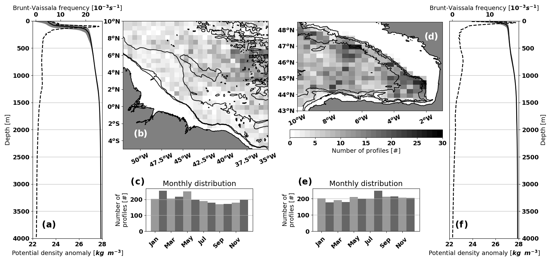
Figure 1Characteristics of the in situ profiles used from the CORA V4.3 dataset for the two areas of interest: (a–c) the western equatorial Atlantic and (d–f) the Bay of Biscay. Panels (b, d) present the spatial distribution of the profiles within boxes of 60 km × 60 km for (b) and 30 km × 30 km for (d). Panels (c, e) present the monthly distribution of the profiles. Panels (a, f) present the mean and the 90 % interval (gray patch) of the potential density anomaly (solid line) as well as the buoyancy frequency (dash line). The potential density anomaly is calculated with a reference depth at the surface.
The typical density profiles derived from the clusters are compared with seasonal means (based on the mean of 3 months; hereafter called 3-month means), averaged over the two areas of interest and processed from the same dataset. In addition the clusters are compared with existing climatologies, also averaged over the two areas. For the Bay of Biscay, BOBYCLIM is used (Bay Of BiscaY's CLIMatology; Charraudeau and Vandermeirsch, 2006; produced by the Ifremer 3). This seasonal climatology uses the profiles in this area from 1862 to 2006 classified into four seasons (3-month means), using a grid of ∘. For both the western equatorial Atlantic and the Bay of Biscay, the ISAS13 climatology is used (In Situ Analysis System; Gaillard, 2015; provided by Copernicus and SEANOE). This monthly climatology is based on the CORA database and averaged from 2004 to 2014, using a grid of ∘. The seasonal climatology of ISAS13 is built using 3-month means.
The potential density and buoyancy frequencies are calculated from TEOS-10 definitions (Millero et al., 2008) that use the Gibbs Sea Water (GSW) equations of Feistel (2003, 2008) (Python GSW package4). Figure 1 presents the distribution of the dataset for the two areas of interest. In the western equatorial Atlantic area, the main stratification occurs around 100 m (Fig. 1a). Most of the variability of the profiles is around this depth but also at the surface. Then, stratification remains constant down to 1500 m and slightly decreases close to the bottom. Note that the spatial distribution of the profiles is not homogeneous, less profiles being available along the shelf break. In the Bay of Biscay area, the stratification is weaker than for the western equatorial Atlantic (Fig. 1f). The strongest stratification and the largest variability occur at the surface. This pattern expresses the dominance of the radiative forcing in this region. Around 750 m, a permanent stratification can be observed. This particular pattern is present in the study of Pichon and Correard (2006) and further detailed in Pairaud et al. (2010). The spatial distribution of the profiles is quite homogeneous in this region.
2.2 Methodology of the classification
Traditionally, the background stratification is classified using either 3-month means or monthly means. Such a method can mix very diverse profiles, leading to vertically smoothed mean profiles. Multiplying spatial boxes and reducing the time interval helps to detail the variability but increase the number of typical profiles considered. The clustering methods are based on the similarity of the profiles with each other to calculate an optimal classification, without being affected by the spatiotemporal variability of the profiles.
For that purpose, a matrix of distance between every profile is built based on the principal component analysis (PCA; Python SciKitLearn decomposition package; Pedregosa et al., 2011) of each profile along two components. The first axis (PC1) is mainly controlled by deep pycnoclines, whereas the second axis (PC2) is mainly controlled by the surface ones. The method provides a 2D space where all the profiles can be represented, called the PCA manifold; thus the distance between each profile can be easily calculated within such a space.
The profiles used for the calculation need to meet some requirements. As the maximum depth of the profiles influences the PCA, the profiles used for the classification have to be defined up to 300 m for the Bay of Biscay and 600 m for the western equatorial Atlantic, where the major variability happens. The measurements have more uncertainties at the surface, so the measurements above 10 m are neglected. The typical density profiles will be used in a frequency domain tidal model (see Sect. 3.1), so only the statically stable density profiles are processed. The threshold used to define an unstable profile is when there are more than two consecutive occurrences of kg m−4 (with δzρ the vertical density gradient). The selected profiles must have more than five measurements over 100 m. In order to run faster algorithms, the profiles need to be on the same vertical grid and without any missing values. Thus, the density profiles are linearly interpolated to fill all the gaps and get all the profiles on a vertical grid of 1 m resolution.
The classification of the profile from the PCA manifold is made using the Ward method (Ward, 1961; Ward and Hook, 1963) based on the 16 nearest-neighbor profiles to build six clusters. A wide range of sensitivity tests have been made to choose the best method and the best parameters; they can be found in Supplement A. The number of clusters needed to represent the variability is complex to set and no proper formulation has actually been found. A high number of clusters leads to having some clusters with few profiles. Thus, for both areas, six clusters is a good compromise that enables us to discuss the density profile variability while keeping well-represented clusters (more than 100 profiles).
Once the classification is done, the typical profile from each cluster is calculated in order to use it as a forcing in the simulations (see Sect. 3.1). The density profiles need to be stable and defined from 0 to 4000 m depth.
Because most of the profiles used for the classification are not defined that deep, the completion process is detailed here. The median of the profiles within the clusters is used as deep as possible. The standard deviation below 1000 m is very weak (Fig. 1a and f) so the profile can be completed with the median of the profiles from the other clusters. If the profile does not reach 4000 m, then the bottom of the profile is extrapolated using the density gradient of the deepest four measurements. The density gradient used for the extrapolation needs to be weaker than kg m−4, which is a common gradient at such a depth.
The median profile is smoothed with a Gustafsson filter (Gustafsson, 1996) of order 3 at 20 m using a forward–backward method (Python SciPy signal package5). The values are sorted to insure the profile is strictly stable, and then the profile is interpolated on a final grid with variable vertical resolution Δz (in meters):
2.3 Application to the two areas of interest
2.3.1 Stratification of the western equatorial Atlantic
The clustering method is performed on the western equatorial Atlantic profiles and the six clusters (designated WEA- followed by a number) are sorted by the number of profiles they gather. The density profiles are measured from 1984 to 2015. The distribution of the 2421 profiles into the six clusters is detailed in Table 1. Note that WEA-4 and WEA-5 have fewer profiles than the other clusters.
Table 1Composition of the clusters and the characteristics of their stratification maximum for the western equatorial Atlantic and the Bay of Biscay. The depth of Nmax corresponds to the maximum of the buoyancy frequency.
Figure 2d illustrates the median of the different typical profiles obtained for each cluster. WEA-6 contains only the density profiles that are exceptional: those 17 profiles show an offset of 1 kg m−3 over the entire depth and were measured during the same period (from October 2005 to March 2006), equally spaced by almost 10 d (Fig. 2e). These measurements were made by a single Argo float (WMO number: 41953). This Argo float failed its salinity measurements for cycles 150–152 and 166–180 (except the cycle 176), which explain the bad calculation of the associated density.
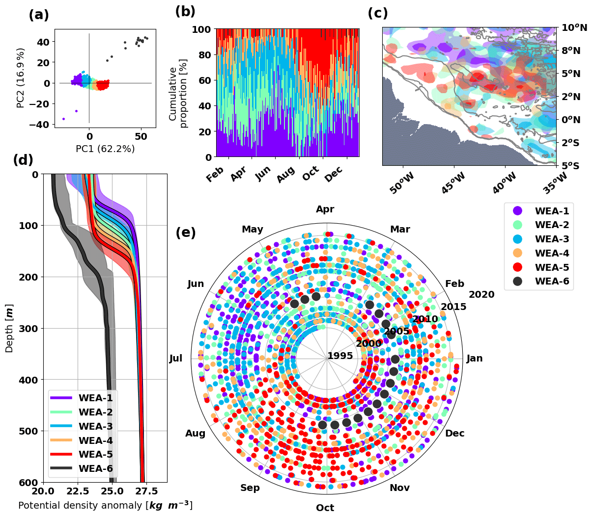
Figure 2Classification of density profile in the western equatorial Atlantic into six clusters: (a) the PCA manifold of the profiles, (b) the cumulative proportion of the clusters during a mean year, (c) the spatial distribution, (d) the median and the 90 % interval of each cluster, and (e) the measurement dates of the density profiles (the angles represent the day of the year, the distance from the center and the year of measurement). The colors of the clusters are common to all the graphs. The colored contours of (c) are set to highlight the areas gathering from two to five profiles (light color) and over five profiles (bold color) for each cluster. The gray contours of (c) show the 200, 1000 and 4000 m isobaths.
The clustering method is efficient enough to detect the exceptional profiles that pass the standard quality control and can be used as a tool to filter them out. As these profiles are less numerous, they will form the last cluster of the classification (WEA-6). From now on, the cluster WEA-6 is neglected, and gathering the suspicious profiles in WEA-6 helps to sort the data and analyze only the realistic profiles contained in the other clusters.
The variability of the western equatorial Atlantic profiles is dominated by the depth of a single pycnocline (Fig. 2d). This variability corresponds to the large 90 % interval observed in Fig. 1a, so this classification does capture the realistic variability of the density profiles. The median value of the upper surface density is centered around 1023.3 kg m−3 for all the clusters. Only WEA-1 and WEA-3 show a greater variability at the surface with the 90% interval (1021.7–1023.9 and 1022.1–1023.6 kg m−3). All the typical profiles have a maximum buoyancy frequency within the same range (Table 1), only the depth of the single pycnocline differs. So, these clusters represent a good framework to investigate the influence of the depth of a single pycnocline on the ITs.
The clusters are not strictly defined during a specific season but rather during the whole year (Fig. 2b and e). In addition, the spatial distribution of the clusters is not homogeneous within the area highlighting spatially bound ocean processes responsible for some specific stratification. The depth of the single pycnocline is highly controlled by the circulation, so the complex spatiotemporal variability of the clusters refers to the complex spatiotemporal variability of the circulation in this region. The cluster classification enables us to focus on a simple parameter (the pycnocline depth) that would be smoothed with a classical seasonal average classification.
WEA-1 is the cluster with the shallower pycnocline depth around 70 m. From September to January and north of 5∘ N, this cluster corresponds to the Amazon river plume (Ffield, 2005, their Fig. 10). From May to July and south of 5∘ N, this cluster corresponds to the North Equatorial Current (NEC, Richardson and Reverdin, 1987). The duality of this cluster is confirmed by the spatial distribution of the seasonality (Fig. A1a).
The other clusters correspond to the seasonality of the North Brazil Current (NBC), mainly influenced by wind-driven eddies from August to November that enhance the retroflection of the NBC water masses into the North Equatorial Counter Current (NECC, Johns et al., 1998). WEA-2 and WEA-3 gather the profiles with a pycnocline depth from 80 m (WEA-3) to 110 m (WEA-2) that correspond to the steady state of the NBC, without the eddies. WEA-4 and WEA-5 gather the profiles with a pycnocline depth deeper than 120 m, mostly from August to November, so they capture the deepening of the single pycnocline due to the large anticyclonic eddies of the NBC.
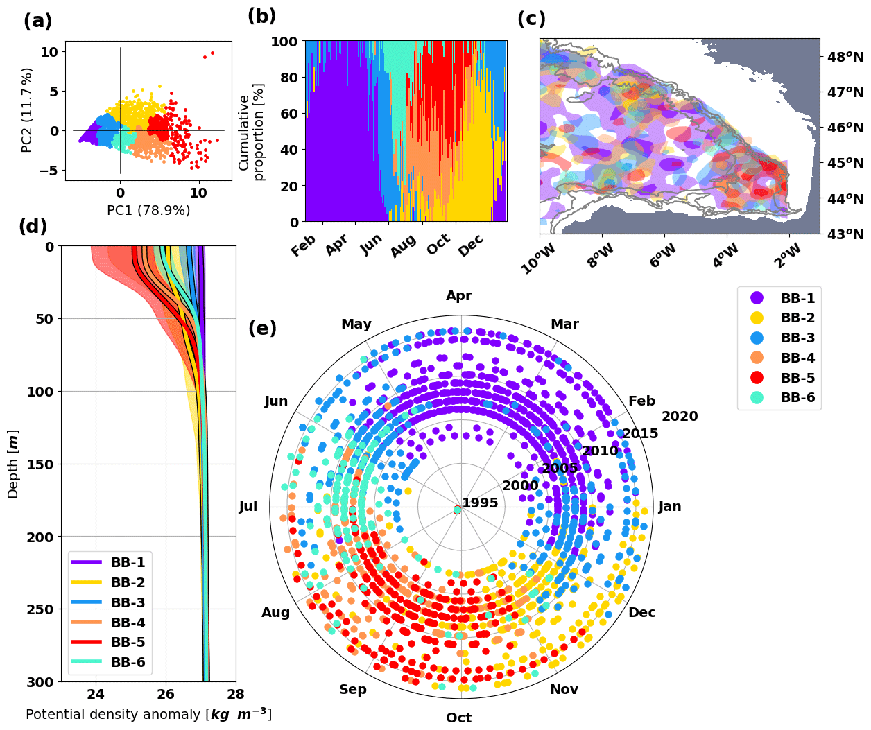
Figure 3Classification of density profile in the Bay of Biscay shelf into six clusters: (a) the PCA manifold of the profiles, (b) the cumulative proportion of the clusters during a mean year, (c) the spatial distribution, (d) the median and the 90 % interval of each cluster, and (e) the measurement dates of the density profiles (the angles represent the day of the year, the distance from the center and the year of measurement). The colors of the clusters are common to all the graphs. The colored contours of (c) are set to highlight the areas gathering from two to five profiles (light color) and over five profiles (bold color) for each cluster. The gray contours of (c) show the 200, 1000 and 4000 m isobaths.
Garraffo et al. (2003) studied the same area looking at the different transport of water using a regional model. They separated the area into four sub-domains (Garraffo et al., 2003, Fig. 11c), where two of them correspond to the area considered in the present study. They highlight that the sub-domain of WEA-2 to WEA-5 (Garraffo et al., 2003, green in Fig. 11c) is influenced by the southern waters coming from the NBC. The sub-domain of WEA-1 (Garraffo et al., 2003, pink in Fig. 11c) is more influenced by the NECC waters than the NBC waters. The cross-shelf transect from mooring measurements (Garzoli et al., 2004, Fig. 2 around 47∘ W) clearly shows the separation of NBC water masses, along the shelf, and the NECC water masses off the shelf. The isopycnals' depth shows a difference of 100 m between the two waters. This difference is comparable to the difference in pycnocline depth observed between WEA-1 around 70 m and WEA-4 and WEA-5 around 140 m. Goni and Johns (2003) used a two-layer model to convert altimetric SSH to the upper layer thickness. The authors show that the anticyclonic eddies in the NBC could increase the upper layer thickness from 20 to 40 m (Goni and Johns, 2003, Fig. 10). This difference is comparable to the difference of the pycnocline depth observed between WEA-2 and WEA-3 around 100 m and WEA-4 and WEA-5 around 140 m.
2.3.2 Stratification of the Bay of Biscay
The clustering method is also performed on the Bay of Biscay profiles. The six clusters are sorted by their number of profiles. The density profiles are measured from 1991 to 2015. The distribution of the 2447 profiles into the six clusters can be found in Table 1. In this dataset, no suspicious profiles are detected with the clustering method, so all of the clusters will be used for the density study. Note that BB-1 has the most profiles, BB-6 has the least and the other clusters are almost equally represented.
Figure 3d shows the six typical profiles processed from the six clusters. In this area, the main variability of the profiles is dominated by the upper surface density. BB-2 and BB-6 are the only clusters to have almost the same surface density. The difference between these two clusters is the depth of this secondary pycnocline (the main permanent pycnocline being at 750 m).
Figure 3b and e highlight that the classification corresponds to the seasonality of the profiles. Chronologically, BB-1 corresponds to winter and spring conditions with deep mixed layers with quasi-homogeneous density profiles. BB-6 corresponds to early summer with density profiles that linearly decrease up to the surface. BB-4 and BB-5 correspond to late summer and early autumn conditions with the most stratified profiles. Finally BB-2 closes the loop corresponding to late autumn with deep surface layer profiles. BB-4 and BB-5 cover the same period simultaneously and the differences are due to the intensity of the stratification: BB-4 corresponds to mild summer stratification generally in July–August, and BB-5 corresponds to stronger summer stratification with more profiles in September–October.
There is also a transitional group, BB-3, composed of profiles from both before and after BB-1 (winter): in December and in May. BB-3 is designated as the shoulder season in the rest of the study. These profiles also occur during late winter corresponding to some warming events that start to build a surface stratification without establishing it.
The spatial distribution shows the clusters are almost equally distributed in the area (Fig. 3c). This result confirms that the variability of the density profiles is dominated by radiative forcing rather than complex changing circulation patterns in this region.
As expected, the clustering methods do identify the seasonality contained in the midlatitude variability. This classification separates the seasonal changes more distinctly than 3-month means: BB-1 lasts for 4 months, BB-6 lasts for 1 month, BB-4 and BB-5 last for 3 months simultaneously, and BB-2 lasts for 2 months. Further comparisons are shown in the next section.
2.4 Discussion
The stratification in the two areas of interest is driven by very different forcing: the Amazon plume and the circulation for the western equatorial Atlantic and the radiative forcing for the Bay of Biscay. The stratification variability due to the circulation is spatially bound, whereas the one due to radiative forcing affects the area homogeneously. The methodology proposed enables us to distinguish the specificity of each sub-region at once.
In this section, some typical profiles from the clusters will be compared with seasonal climatologies (ISAS13 and BOBYCLIM) and to the 3-month means made from the CORA V4.3 dataset. For the western equatorial Atlantic, the two extreme clusters are chosen. WEA-1 is compared with the spring mean because this is the season with the shallower pycnocline and because this cluster is highly represented in spring. WEA-5 is compared with the fall mean because this is the season where this cluster occurs the most. For the Bay of Biscay, BB-2, BB-4 and BB-5 are used to investigate the influence of fewer months in the classification and to discriminate between mild and stronger events. BB-2 is compared with the fall mean, and BB-4 and BB-5 are compared with the summer mean.
The climatology profiles are averaged in the same areas and smoothed following the method explained in Sect. 2.2.
For the western equatorial Atlantic area, Fig. 4a and b show that ISAS13 seasonal profiles are smoother than the CORA V4.3 seasonal profiles, likely due to the spatial and vertical smoothing used in the climatology. The climatology profiles show a slightly smoother pycnocline than the cluster profiles (Fig. 4a and b). Thus, the averaging of the large diversity of the profiles within one season tends to smooth the stratification and does not represent it as well as the cluster classification. WEA-1 and WEA-5 both represent a more contrasted part of the 90 % interval of the seasonal profiles considered (gray patch). WEA-1 sets the upper limit of the 90 % interval of the spring climatology (Fig. 4a). WEA-5 sets the lower limit of the 90 % interval of the fall climatology (Fig. 4b). Still, the median of both clusters is part of the seasonal 90 % interval, indicating that the clusters represent a right proportion of these seasonal profiles.
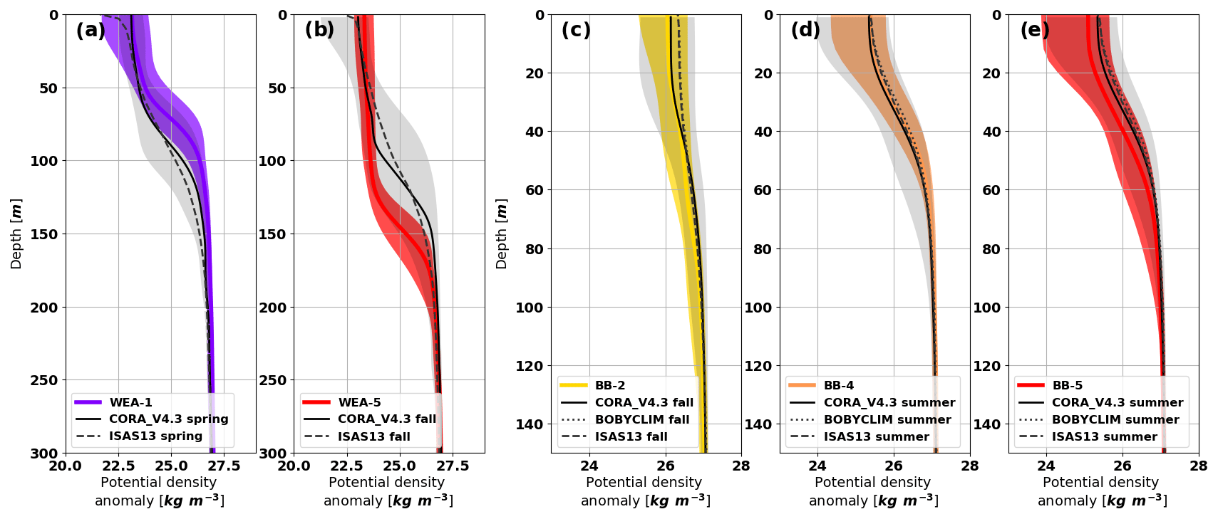
Figure 4Climatology profiles compared with the corresponding selected typical profiles from the cluster classification: the western equatorial Atlantic (a) WEA-1 and (b) WEA-3 and the Bay of Biscay (c) BB-1, (d) BB-4 and (e) BB-5. The gray shadings are the 90 % interval calculated from the CORA V4.3 dataset using seasonal classification, and the colored shadings are the 90 % interval of each cluster.
These 3-month means do not highlight the profile variability as well as the cluster classification do. The western equatorial Atlantic has a strong spatial variability (Fig. 2c), which explains why averaging classifications are not effective. The 3-month mean is not recommended for this area that has complex circulation, mixing processes and a low dependency to radiative forcing.
For the Bay of Biscay area, the BOBYCLIM and ISAS13 climatologies are almost identical for the fall and summer seasons. The fall climatology profiles of CORA V4.3 and BB-2 profiles are very close (Fig. 4c); the overlap of both 90 % intervals is high, validating that BB-2 corresponds to the fall climatology. The BB-4 median profile exactly fits the summer climatology profile (Fig. 4d). The 90 % interval of the BB-4 shows more stratified profiles than the summer climatology ones, especially shallower than 40 m. The BB-5 profiles are indeed more stratified than the mean summer climatology profile but better fit the 90 % interval of the climatology deeper than 40 m that are not represented by BB-4 (Fig. 4e). The main difference between the BB-4 and BB-5 is not only located at the surface but also around 60 m where the two 90 % intervals of the clusters do not overlap each other. BB-4 and BB-5 contribute to different parts of the summer climatology 90 % interval and enable us to separate two stratification patterns that are mixed within the classical 3-month mean.
The cluster classification is more effective than the 3-month mean to distinguish the different stratification regimes that can occur within a given time period. The cluster analysis enables us to describe different pycnocline states: established or transitory states and mild or extreme states. In the midlatitude Bay of Biscay, the seasonal radiative forcing is strong and makes the stratification uniform horizontally. There, the six-cluster classification gathers the same amount of information about the seasonality as the 12 groups of the monthly classification. Thus, the cluster classification is a more pithy approach. In the Amazon tropical regions, the spatial variability is more important. This adds complexity to the study of the stratification variability via a time-dependent classification and requires a good knowledge of the region's circulation and water masses. The cluster analysis does not preferably consider time-dependent or space-dependent classification, so this method is far more accurate than climatologies to investigate circulation-driven stratification variability, such as in the tropics.
The clustering classification is used over a long period of time in this study, but doing so does not blur the interannual variability. The long-term variability can be observed looking at the variability within the distribution between the clusters. Figures 2e and 3e can also help to observe such variability. For example, WEA-4 and WEA-5 are usually associated with the period from August to November, but for the year 2006, WEA-4 and WEA-5 are only present from August to September. In a classical seasonal or monthly averaged classification, such long-term variability would have smoothed the stratification profiles. Here, the typical profiles are based on similar instantaneous profiles, ensuring more realistic profiles.
3.1 Model configuration for the IT simulations
The T-UGOm (Toulouse Unstructured Grid Ocean model) has been used to simulate the ITs. Initially developed to resolve the two-dimensional tidal equations (Piton et al., 2020; Lyard et al., 2021a), this model has been extended to resolve the three-dimensional tidal equations in the frequency domain (Nugroho, 2017; Lyard et al., 2021b). The model configuration is set to be hydrostatic and with a free surface. The 3D version uses Lagrangian layers that follow the fluid displacement in the vertical dimension. The experiments are focused on the M2 major tidal component in the two areas of interest and are based on the stratifications described in the previous section. The frequency domain calculation uses the tidal dynamical equations expressed in the complex, frequency space. This allows for much faster computation time than the time-stepping calculation but does not support a stratification evolution over time, and the simulated ocean needs to be at rest. Thus, if the density profile is unstable, high-amplitude instabilities are created because the stratification induces vertical motions rather than acting as a restoring force.
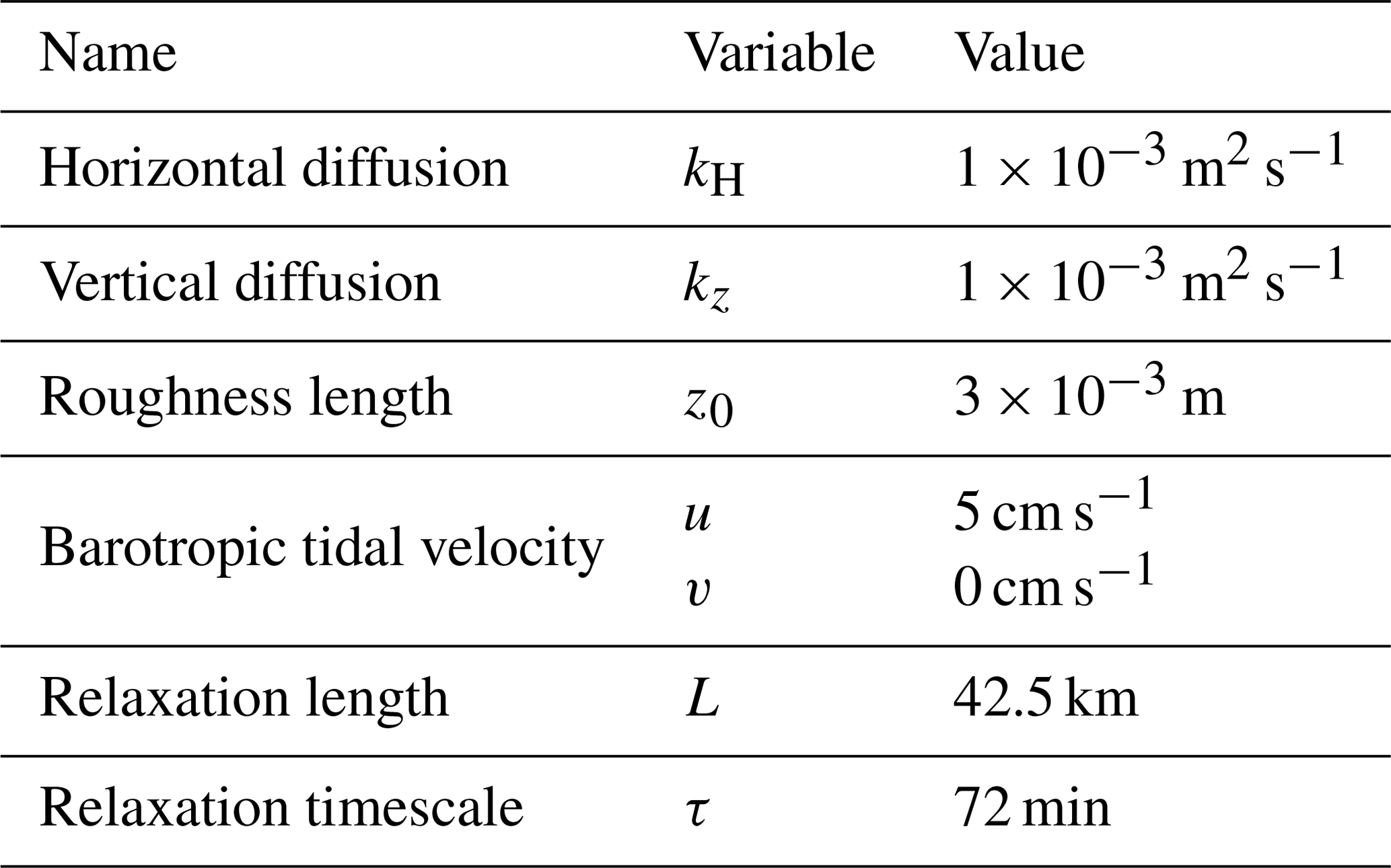
All simulations are carried out with the same configuration and the same inputs that are shown in Table 2. The reference latitude θref for the calculation of the Coriolis parameter is set differently for each area: θref=0∘ N for the western equatorial Atlantic and θref=47∘ N for the Bay of Biscay. This enables us to compare the simulations with IT measurements and realistic simulations. A single density profile is used to set the stratification uniformly over all of the domain. The typical density profiles from the above classifications (Sect. 2.3.1 and 2.3.2) are used and one simulation is made for each profile.
This model is applied using the academic configuration from the COMODO project (Ocean Modeling Community, 2011–2016, PI: Laurent Debreu, Soufflet et al., 2016) for the study of the internal waves generated on a continental slope (Nugroho, 2017). The project was originally built to compare different ocean models and T-UGOm 3D was one of them. The original configuration is based on the configuration of Pichon and Maze (1990): a flat-bottom ocean of 4000 m depth in the abyss (on the left) and 200 m depth on the shelf (on the right); the domain is 880 km wide along the axis x and the size of one horizontal mesh (1 km) along y axis. The slope is defined as
where b is the bathymetry, x0=426 km, x1=443 km, x2=479 km and x3=484 km. This bathymetry is similar to an averaged continental slope (the comparison to realistic bathymetry of the two areas of interest is shown in Fig. B1). The domain is described by 1760 finite-element triangles using the LGP1×LGP0 convention. LGP1 refers to the summit of the triangles where the pressure and elevation are set continuously from one triangle to another (Lagrange finite element of 1 degree of freedom). LGP0 refers to the barycenter of the triangle where the velocity is set (Lagrange finite element of 0 degree of freedom). In the vertical dimension, density is piecewise linear (i.e., linear inside layers with possible discontinuities at the layers' interfaces), and velocity is uniform. The model is based on the primitive momentum equations, continuity equation and density advection equation. The model unknowns are the level displacements (including the free surface), horizontal velocities and density anomalies (due to advection in layers). However, a 3D wave-equation approach allows us to form a linear system where unknowns are limited to level displacements and density anomalies, with velocities then being deduced once the 3D wave-equation system is solved.
This configuration places the slope in the center of the domain which limits the study of off-shelf IT propagation that presents longer wavelengths than the on-shelf IT propagation. This configuration only allows us to resolve around 2 or 3 times the wavelength in the abyssal domain, whereas more than 20 or 30 times the wavelength is resolved in the shelf domain. To compensate for this difference, the slope is shifted toward the shelf by 220 km. This allows us to resolve around 4 or 5 times the wavelength in both domains.
In the vertical, 80 σ layers (which follows the bathymetry) are distributed using a cosine function between 0 and . This vertical distribution enables us to better represent surface pycnocline and the associated ITs than a uniform distribution.
The von Kármán–Prandtl equation is used to calculate the bottom velocity affected by the bottom friction, as described for the AMANDES tidal model in the Amazon estuary (Le Bars et al., 2010). Using a frequency domain calculation, there is no spin-up of the simulation that could lead to a stable value of the bottom friction. So, an iterative process is used in order to make the bottom velocity converge, solving the equations four times, each time using the previous bottom velocity. The model uses logarithmic buffer areas at the open boundaries (both sides) in order to stabilize the results. The relaxation term R is expressed as follows:
with τ=72 min being the relaxation timescale, d the distance from the boundary and L=42.5 km the relaxation length.
In order to separate properly the baroclinic tides (ITs) from the barotropic tides, the solution is decomposed into vertical modes following the methods described in Nugroho (2017). For the following discussion, mode 1 and higher will refer to vertical baroclinic modes, whereas mode 0 will refer to the vertical barotropic mode.
3.2 Modeling results on the two areas of interest
3.2.1 Impacts of the western equatorial Atlantic stratifications
The typical profiles from the western equatorial Atlantic have almost the same maximum buoyancy frequency, so only the depth of the single pycnocline differs in this area. From now on, these cluster profiles will be sorted by the depth of the single pycnocline: WEA-72 m, WEA-88 m, WEA-108 m, WEA-128 m, WEA-148 m (corresponding to WEA-1, WEA-3, WEA-2, WEA-4, WEA- 5; Table 1).
We will first discuss the impact of the depth of a simple pycnocline on the vertical modal structure (Fig. 5 left panels), starting with w and η. For mode 1, the deeper the pycnocline, the further the mode is shifted toward the surface. For mode 2, the deeper the pycnocline, the further the mode is shifted toward intermediate layers: the first extremum is deeper and the second one is shallower. For mode 3, the pycnocline depth only affects the first extremum: with a deeper pycnocline, the extremum is deeper. The same observation can be made for the vertical modal structures of u, v and P. At the surface, for a deeper pycnocline, mode 1 is stronger and the higher modes are weaker. The impact of the depth of a single pycnocline on the mode shifts seems to be linear for modes 1 and 2.
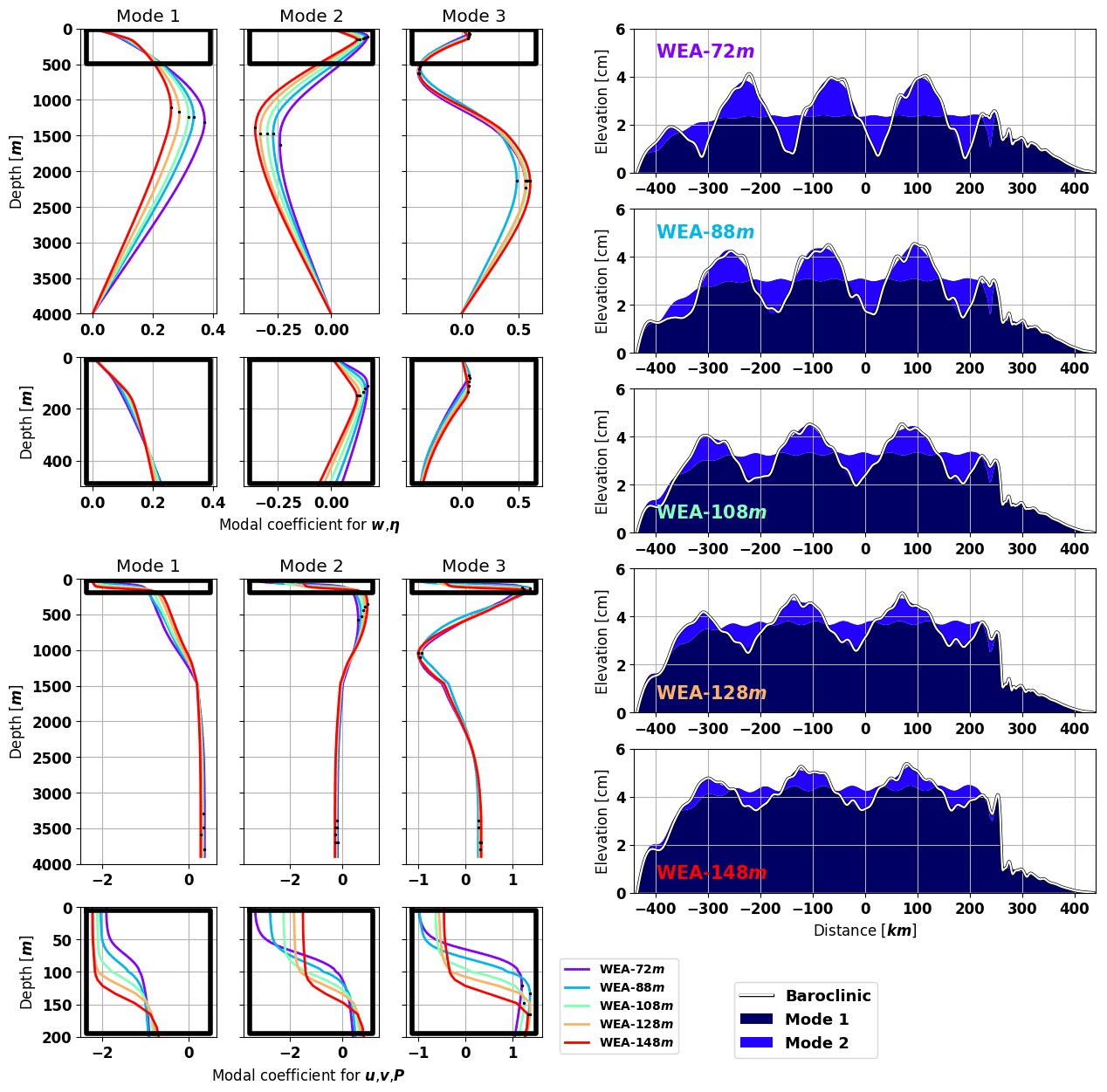
Figure 5Baroclinic modal structures for the three first modes (left panels) and simulated amplitude of baroclinic surface elevation for the five first modes (right panel) for all the typical density profiles of the western equatorial Atlantic. The vertical modal structures are different for vertical processes (w and η, upper left panels) and horizontal ones (u, v and P, lower left panels). The black points show the extrema of the modes. The simulations are sorted with respect to the depth of the pycnocline. On the right panels, the white line represents the sum of the baroclinic modes and the colored patches represent the modal contribution to the complex sum: if the patch of mode n is located on top of the sum line, then mode n works against mode n−1.
The only exception to this pattern happens for mode 3 (u, v, P) at the surface: WEA-72 m and WEA-88 m have the same amplitude, whereas WEA-88 m was expected to be weaker and to be sorted between WEA-72 m and WEA-108 m such as for modes 1 and 2. This difference can be due to small density differences at the surface between the typical density profile of about 0.02 kg m−3, which is the smallest difference at the surface between the clusters.
Figure 5 (right panels) illustrates the simulated amplitude of the baroclinic surface elevation. For the western equatorial Atlantic simulations, the overall amplitude of the baroclinic elevation scales from 4 to 5 cm with negligible contribution of the modes higher than 2. When the single pycnocline deepens, the total amplitude of the elevation increases with a dominance of mode 1 over mode 2. The ITs' horizontal wavelength seems to be larger with a deeper pycnocline.
To investigate this impact, the wavelength of each mode has been calculated for the abyssal domain (from −300 to 200 km). The wavelength is calculated following the method of Welch (1967) with 200 elements per segment and a zero padding of 5000 elements. Using the zero padding enables us to increase the resolution of larger wavelengths but creates irrelevant wavelengths, so all the wavelengths larger than 500 km are ignored (λmax=Ndx).
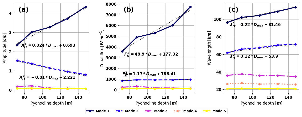
Figure 6(a) Surface elevation amplitude, (b) vertically integrated zonal energy flux and (c) horizontal surface wavelength for each vertical mode with respect to the pycnocline depth. The calculations are based on the western equatorial Atlantic simulations over the abyssal domain (−300 km < x < 200 km). The fit equations for the two first modes are shown below the curves (with the IT surface amplitude for mode n, the IT surface wavelength for mode n and Dmax the pycnocline depth).
Figure 6 presents the IT elevation amplitudes, the vertically integrated energy fluxes and the horizontal surface wavelengths of each baroclinic mode with respect to the depth of the single pycnocline. As expected with the shape of the modal structures, modes 1 and 2 are linearly controlled by the depth of a single pycnocline. A deep pycnocline increases the IT generation and the associated energy flux, which doubles between WEA-72 and WEA-148 m. The variability of the energy flux only affects mode 1, and mode 2 presents almost the same energy for all the simulations. The elevation amplitude variability affects both mode 1, which increases with a deep pycnocline, and mode 2, which lowers with a deep pycnocline. This means that the energy of mode 2 is shifted away from the surface as the single pycnocline deepens.
A deep pycnocline also increases the horizontal surface wavelengths of modes 1 and 2 with a stronger impact on mode 1. This can lead to a strong aliasing of the IT corrections and altimetric observations if this variability is not taken into account. For example, the wavelength difference for mode 2 between WEA-71 and WEA-148 m is about 10 km. With only three occurrences of the wave beam at the surface, the shift associated with mode 2 is about 30 km. The correction that only uses a wavelength of 60 km to correct mode 2 (corresponding to WEA-71 m) will be in phase opposition after only three occurrences if the stratification leads to an actual wavelength of 70 km (corresponding to WEA-148 m). This rough calculation helps to understand why small changes in the wavelength can completely change the shape of the surface IT signature.
Tchilibou et al. (2020) reported a similar observation comparing two simulations from El Niño and La Niña situations in the Solomon Sea. In this region, the El Niño stratification is characterized by a shallow pycnocline and the La Niña stratification is characterized by a deep pycnocline. The authors pointed out that this stratification variability is one of the sources of the non-stationarity of the ITs observed using long-term altimetric SSH. The surface elevation of the model outputs seems to present a larger horizontal surface wavelength during La Niña than during El Niño (Tchilibou et al., 2020, Fig. 8).
In the western equatorial Atlantic area, the high dependency of the horizontal surface wavelength and the ratio between modes 1 and 2 to the depth of a single pycnocline could be a major contribution to non-stationary ITs that appear in the study of Zaron and Ray (2017). These results reinforce the importance, in the future, of properly taking into account the stratification regimes in the IT correction and especially when a single pycnocline controls the variability of the stratification. Empirical relations for modes 1 and 2 are proposed by fitting the curves and could be useful to determine the ITs' surface patterns in order to properly correct the non-stationarity of the ITs. Other tests should be made in order to integrate slope properties and barotropic current into these empirical relations.
3.2.2 Impacts of the Bay of Biscay stratifications
In this section, the clusters are sorted following the period of the year they represent: BB-1, BB-3, BB-6, BB-4, BB-5 and BB-2. To facilitate the description, the clusters are renamed after the corresponding season: BB-winter, BB-shoulder, BB-spring, BB-summer, BB-hot-event and BB-fall.
In the Bay of Biscay case, the differences between the typical profiles are not driven by the depth of the secondary pycnocline but by the buoyancy frequency in the upper surface layer (<25 m, Fig. 3b). Indeed, the maximum value of N has great variability, whereas the depth of the secondary pycnocline is always close to 40 m (Table 1). Because of the variability in N, the interpretation of the stratification impacts on the baroclinic modes (Fig. 7, left panels) is more complex than for the western equatorial Atlantic simulations. The easiest way to proceed is to describe the seasonal impact mode by mode.
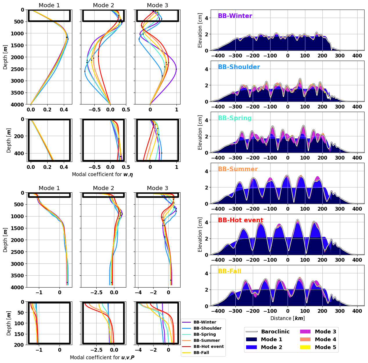
Figure 7Baroclinic modal structures for the three first modes (left panels) and simulated amplitude of baroclinic surface elevation for the five first modes (right panel) for all the typical density profiles of the Bay of Biscay. The vertical modal structures are different for vertical processes (w and η, upper left panels) and horizontal ones (u, v and P, lower left panels). The black points show the extrema of the modes. The simulations are sorted with respect to the seasons. On the right panels, the white line represents the sum of the baroclinic modes and the colored patches represent the modal contribution to the complex sum: if the patch of mode n is located on top of the sum line, then mode n works against mode n−1.
Mode 1 is almost the same for all the clusters for the vertical modal structure of (w, η) and (u, v, P). So mode 1 is not sensitive to the variability of the stratification because it strongly depends upon the constant maximum at 750 m (Fig. 1f).
Mode 2 presents the same pattern for the vertical modal structures of (w, η) and (u, v, P): the more stratified the secondary pycnocline is, the further the mode is shifted toward the surface. The clusters are sorted as follows: BB-shoulder, BB-spring, BB-fall, BB-summer and BB-hot-event. BB-winter is excluded from this pattern.
For mode 3 (w, η) at the surface, the pattern is the opposite of mode 2: BB-hot-event, BB-summer, BB-fall and BB-spring. BB-winter and BB-shoulder are excluded because they are weaker than BB-hot-event. For mode 3 (u, v, P) at the surface, the pattern is completely different: BB-winter, BB-shoulder, BB-hot-event, BB-fall, BB-summer and BB-spring. This could be due to the stratification at the surface (Fig. 3d).
The overall baroclinic amplitude of the surface elevation ranges between 2 and 4 cm (Fig. 7 right panels). Modes 1 and 2 are stronger with the increase in stratification between 20 and 60 m: 1.7–0.3 cm for BB-winter and 2–1.5 cm in the highly stratified BB-hot-event. Mode 2 is more sensitive to stratification: it is almost equivalent to mode 1 for BB-hot-event, whereas it is almost null for BB-winter. Mode 3 is stronger during BB-shoulder, BB-spring and BB-fall than for other stratification, where it is almost null. This confirms the observations made for the modal structures. Modes 4 and 5 are only visible during BB-shoulder.
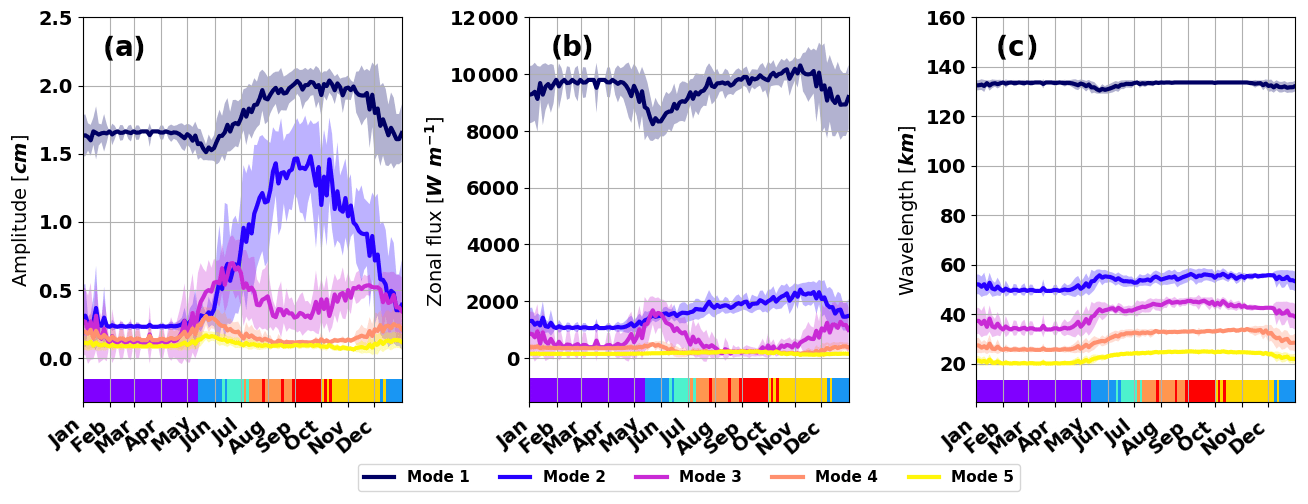
Figure 8Weighted mean of (a) the surface elevation amplitude, (b) the vertically integrated zonal energy flux and (c) the surface wavelength for each vertical mode during the year. The calculations are based on the Bay of Biscay simulations over the abyssal domain (−300 km < x < 200 km). The climatology is built with a time step of 3 d where the ratio of each cluster is used as the weight. The shading represents the weighted standard deviation. The ruler at the bottom of the plots shows the color of the dominant cluster along the year.
In summary, for the elevation amplitude in the Bay of Biscay, mode 1 is controlled by the maximum of N at 750 m, mode 2 is controlled by the value of N between 20 and 40 m, and mode 3 might be controlled by the value of N between the surface and 20 m. So the depth of the pycnoclines is not the only parameter representing the IT variability in this area. As no adequate proxy has been actually found, the IT elevation amplitudes, energy fluxes and horizontal surface wavelengths are processed seasonally. A climatology has been developed with a time step of 3 d. The values of each mode are calculated from the weighted mean of the cluster distribution in the dataset over a window of 3 d along the year. The weighted standard deviation is also calculated to evaluate the variability inside each time step.
Figure 8 shows this climatology; to simplify the descriptions, BB-winter values are used as a reference for the comparisons. The elevation amplitudes are the most contrasted through the year. Mode 1 is stronger from August to October with a homogeneous value of 2 cm through this period. It became weaker in May (around 1.5 cm) and maintains a plateau of 1.7 cm from December to May. Mode 2 has larger amplitude variability compared with other modes. From 0.3 cm in winter and spring, it increases to 1.5 cm in September and then decreases until January. Even with the elevation amplitude, mode 3 has substantial amplitude variability: two peaks at 0.7 cm and 0.5 cm happen in June and November, otherwise the mode stabilized around 0.2 cm. This particular pattern seems to be due to the stratification near the surface, stronger in BB-shoulder and BB-spring compared with other cluster that are well mixed near the surface. Mode 4 and 5 amplitude patterns are close to the mode 3 one, but the peaks happen in May and December so are mainly caused by BB-shoulder stratification.
The energy fluxes are less affected by the variability of the stratification in the Bay of Biscay than in the western equatorial Atlantic but are stronger. Mode 1 is almost constant through the year, around 10 000 W m−1, and only decreases during May–June and December to around 8000 and 9000 W m−1. Mode 2 increases steadily from winter around 1000 W m−1 to around 2000 W m−1 in November. The mode 3 only rises during May–June and December up to 2000 and 1000 W m−1. Modes 4 and 5 are weaker and follow a similar pattern than mode 3. The seasonality of the Bay of Biscay ITs highlights that mode 3 uses the energy of mode 1 to build up.
The wavelengths have a weak variability between all the simulations, explaining why the standard deviation is almost null. The wavelength of mode 1 is almost constant during the year; it only decreases in May and December, due to BB-shoulder stratification. The wavelengths of modes 2, 3, 4 and 5 have similar pattern around two values: lower from February to May (50, 35, 26 and 20 km) and longer from June to December (56, 45, 33 and 25 km). The shifts are stronger for modes 3 and 4 and are clearly due to the presence of surface stratification after winter.
The set of academic simulations coupled to the clustering analysis enables us to build a climatology of the IT properties in the Bay of Biscay. In this area the permanent pycnocline at 750 m makes mode 1 more stable than in the western equatorial Atlantic. The elevation amplitude and the energy flux highlight a substantial variability of the first three modes along the year. Modes 2 and 3 represent up to one-quarter of the total IT energy flux and up to half of the elevation amplitude in non-winter seasons. Such variability in the proportion of the modes implies that the horizontal scales of the ITs vary along the year leading to substantial non-stationarity in this area.
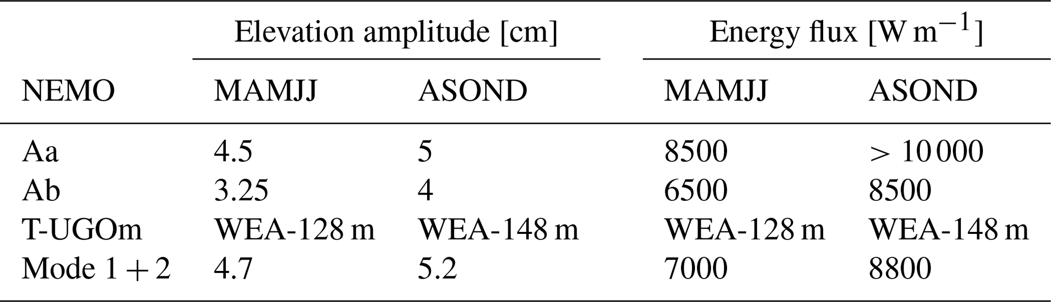
Table 3Baroclinic elevation amplitude and vertically integrated energy flux near the IT generation zone. The NEMO simulation is compared throughout two seasons: from March to July (MAMJJ) and from August to December (ASOND). MAMJJ stratification is close to the WEA-128 m one and ASOND stratification is close to the WEA-128 m one. NEMO values have been extracted on two generation zones near 1∘ N, 45.8∘ W (Aa and Ab in Tchilibou et al., 2021).
3.3 Validation and discussion
To compare the T-UGOm simulations with realistic studies, some atlases of ITs and a realistic NEMO simulation are used. The IT atlases of Ray and Zaron (2016) and Zaron (2019) (HRET V8.1) are built from long-term altimetry harmonic analysis and thus show the stationary part of the ITs for the mean stratification. In the western equatorial Atlantic, the IT elevation amplitude is on the order of 6 cm in Ray and Zaron (2016) and 4 cm in HRET. In the 2015 NEMO simulation of Ruault et al. (2020), the IT surface elevation amplitude is on the order of 5 cm (Tchilibou et al., 2021). With elevation amplitudes ranging between 4 and 6 cm in T-UGOm simulations, the values are similar compared to those altimetry-derived atlases and realistic simulation.
In the Bay of Biscay, the IT elevation amplitude is on the order of 1 cm in Ray and Zaron (2016) and 2 cm in HRET. The elevation amplitudes of T-UGOm, between 2 and 4 cm, are higher compared with those IT atlases but have the right order of magnitude. These differences could originate from the forcing of the barotropic tide, the bathymetric slope and the realistic stratification used within our modeling approach but also from the limitations of these atlases.
As the background stratification was the focus of this study, other parameters have been equally set in the two configurations (western equatorial Atlantic and Bay of Biscay; Table 2). This methodology enables us to compare the different stratification pattern between the two areas of interest and conclude that the variability of the depth of a unique pycnocline (western equatorial Atlantic) leads to a stronger impact over IT surface signature than the variability of secondary pycnoclines near the surface (Bay of Biscay).
The slope of the shelf break of the Bay of Biscay is similar to the one of the simulation but the slope of the western equatorial Atlantic is steeper (Fig. B1). Based on FES-2014b (Lyard et al., 2021a), the M2 tidal barotropic currents are around 3 cm s−1 in the western equatorial Atlantic and around 6 cm s−1 in the Bay of Biscay, whereas 5 cm s−1 has been set in the simulations. Thus the simulations of the western equatorial Atlantic might underestimate the ITs because of the slope but also overestimate them because of the barotropic currents. Finally, the barotropic tides and the bathymetric slope used in the simulations should lead to quite realistic results.
Now, the realism of the IT variability is investigated using the results of the NEMO simulation. The ITs of the NEMO simulation have been studied by Tchilibou et al. (2021) through two seasons: from March to July (MAMJJ), when the NBC does not show eddies, and from August to December (ASOND), when strong NBC rings influence the area. Two major generation sites are highlighted near 1∘ N–45.8∘ W (Aa and Ab). The stratification near these generation sites is similar to WEA-128 m during MAMJJ and WEA-128 m during ASOND (Fig. C1). The stratification of NEMO simulation is weaker than the one observed with the CORA database, but the variability of the depth of the unique pycnocline seems comparable.
Table 3 shows the elevation amplitudes and the vertically integrated energy fluxes near the generation zone for the two seasons. The values from the NEMO simulation show the same pattern highlighted in this study with stronger ITs when the unique pycnocline is deeper (ASOND). The amplitude of the variation between the two seasons is also similar to the variations between WEA-128 and WEA-148 m.
The ITs' stationary horizontal surface wavelength is also extracted from HRET and from the NEMO simulation. The wavelength calculation is made with a 2D fast Fourier transform of the ITs' surface elevation complex field. Using the complex field enables us to extract the direction of propagation in addition to the wavelengths. Because the NEMO simulation only is for the area 2∘ S–9∘ N, 52–43∘ W, the same area is used for HRET.
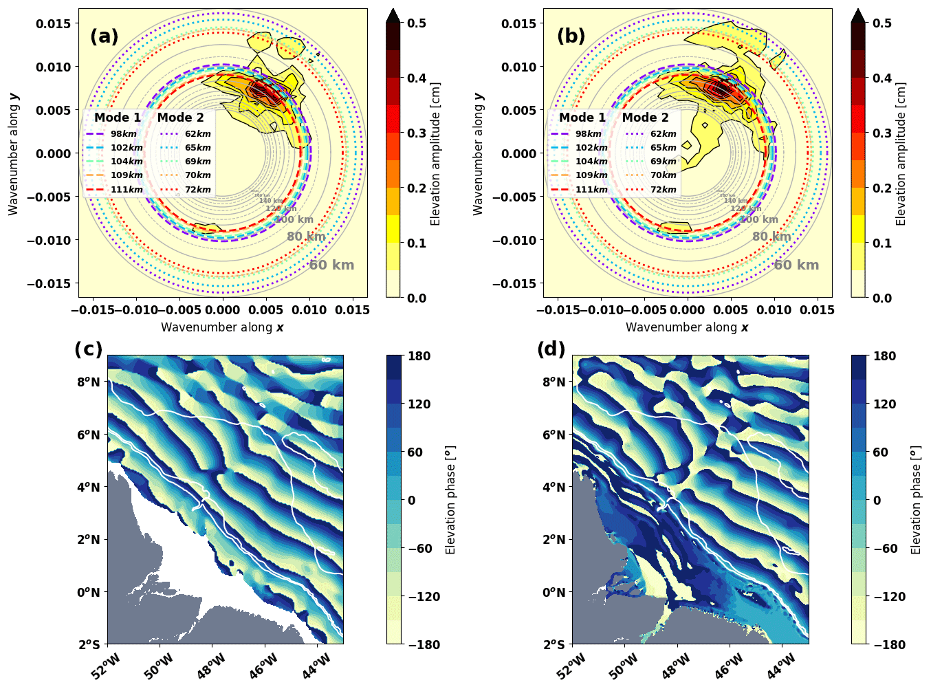
Figure 9Two-dimensional fast Fourier transform of the baroclinic surface elevation for M2 from (a) the HRET V8.1 atlas (Zaron, 2019) and (b) a realistic regional NEMO simulation for 2015 (Ruault et al., 2020) and (c, d) their associated phase field. The gray rings represent the horizontal wavelength grid scale and the colored rings represent the horizontal wavelengths of modes 1 and 2 for the T-UGOm simulations. The value of the wavelengths is shown in the legend.
Figure 9 first shows that the horizontal surface wavelength pattern is very similar between HRET and NEMO. They highlight a major wavelength of 110–120 km propagating northeastward and a secondary wavelength from 70–80 km propagating in the same direction. In NEMO, the propagation of this secondary wavelength is stronger and wider than in HRET. This could be due to the constraints used in HRET to better structure the ITs. The phase field of HRET shows IT propagation with wave crests roughly linear, whereas the NEMO phase field shows them more smoothly curved (Fig. 9c and d).
The horizontal surface wavelengths in HRET and NEMO are coherent with both modes 1 and 2 horizontal surface wavelengths of T-UGOm simulations. The T-UGOm wavelengths are slightly longer, which might mainly originate from the bathymetry differences (4000 m instead of 5000 m) and secondarily from the variability of the depth of the unique pycnocline.
More realistic experiments with various stratifications in a realistic regional grid are presently being carried out for the ITs in the Bay of Biscay with the model SYMPHONY (Marsaleix et al., 2008). So far, these simulations have led to similar conclusions compared to the ones obtained with the T-UGOm academic configuration (Barbot, 2021).
These validations confirm that the T-UGOm simulations, although very academic, are in the right range compared to more realistic cases. Such idealized simulations are thus a good way to estimate the IT properties before running more realistic but complex 3D simulations. Thus, IT atlases seem to underestimate the ITs generated in the Bay of Biscay and do not show the non-stationarity of the ITs that the T-UGOm simulations suggest (Zaron and Ray, 2017). As the non-stationarity in this area is mainly controlled by modes 2 and 3, this underestimation could originate from the spatial resolution of long-term altimetry which might not be thin enough to resolve the wavelengths of mode 2 and higher. This questions the use of such IT atlases in the future corrections of the SWOT measurements.
The classification of density profiles through clustering methods is very useful to describe both spatial and temporal variability of the stratification. As shown, this methodology can highlight different regimes of stratification that are linked to seasonality (Bay of Biscay) or to both spatiotemporal distributions (western equatorial Atlantic) at the same time. Thus, any kind of stratification variability can be handled with a single methodology. Especially for cases that are not driven by seasonality or for cases with clear spatial distribution variability, this methodology is an improvement compared with the seasonal classification.
The users of such a cluster methodology need to be aware of some specific parameters. The first and more important one is the normalization of the profiles. This choice is important and can change the goal of the classification. The second point is the choice of the clustering method for systematic or automated stratification studies. Many clustering methods exist with different performances, but a first selection can be made by looking at the distribution of the PCA manifold.
For the western equatorial Atlantic, the clusters help to highlight the strong spatiotemporal variability of the stratification and the dominance of the depth of a single pycnocline in this variability. In the Bay of Biscay, the clusters reproduce the seasonality of the stratification and highlight two different regimes for summer season.
The present results of IT simulations allow a better understanding of the IT dependency on the background stratification. This dependency not only occurs in areas where the stratification is driven by the radiative forcing but also in areas where the stratification is driven by the circulation. First, the stratification variability has a stronger impact on ITs if the stratification is composed of a single pycnocline. In the tropics, such stratification is maintained year-round and is stronger than at midlatitudes. Second, the variability of surface layer stratification, mostly driven by the radiative forcing, has a stronger impact on modes 2 and 3. Third, the stratification variability impacts modal distribution and the horizontal surface wavelength, leading to a variability of the horizontal scales of the ITs.
These results will impact future works dedicated to ITs' surface elevation observation and prediction as they suggest that harmonic analysis of long time series underestimates the ITs multi-mode amplitude and omits the IT wavelength of modes 2 and 3. Moreover, without realistic horizontal wavelengths, the ITs' surface elevation corrections based on such methods, could create a fictitious signal in the corrected observations resulting from the difference between the real IT wavelengths and the wavelength of the correction. This approach should be preferably used for regions where the stratification regimes have large spatial and temporal scales, as in the midlatitude areas with weak circulation. The frequency domain modeling proposed in this study could be used to build multiple simulations with various stratification regimes that could then serve as references or constraints for future IT corrections atlases. However, for regions with highly variable stratification regimes and strong circulation, this approach should be used with caution. Such modeling would not be representative of the circulation and could also be highly unstable.
Finally, coupling the two approaches of clustering methods and the academic simulations results in the production of a new type of climatology of the IT elevation amplitudes, energy fluxes and surface wavelengths for the five first baroclinic modes. The efforts to find a formulation to link the IT properties to the stratification need to be pursued for the midlatitudes in order to obtain a parametrization that would unify the different regions of the global ocean.
Currently, the SWOT mission encourages international efforts in order to separate the mesoscale and ITs' surface elevation contributions. This study invites other researchers to carefully consider the background stratification and even more its variability within the different approaches used, in order to predict and remove the ITs' surface elevation signature.
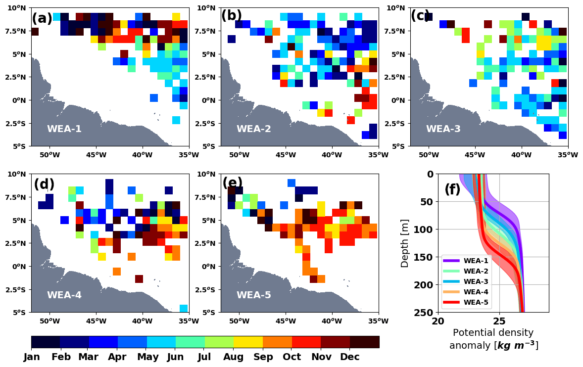
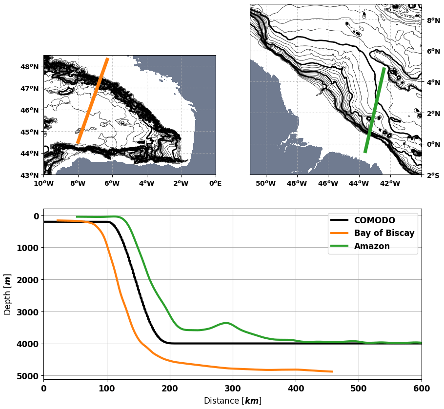
Figure B1Realistic continental slope bathymetry over the two studied areas compared with the COMODO one. The bold contours show the isobaths spaced every 1000 m and the plain ones every 200 m.
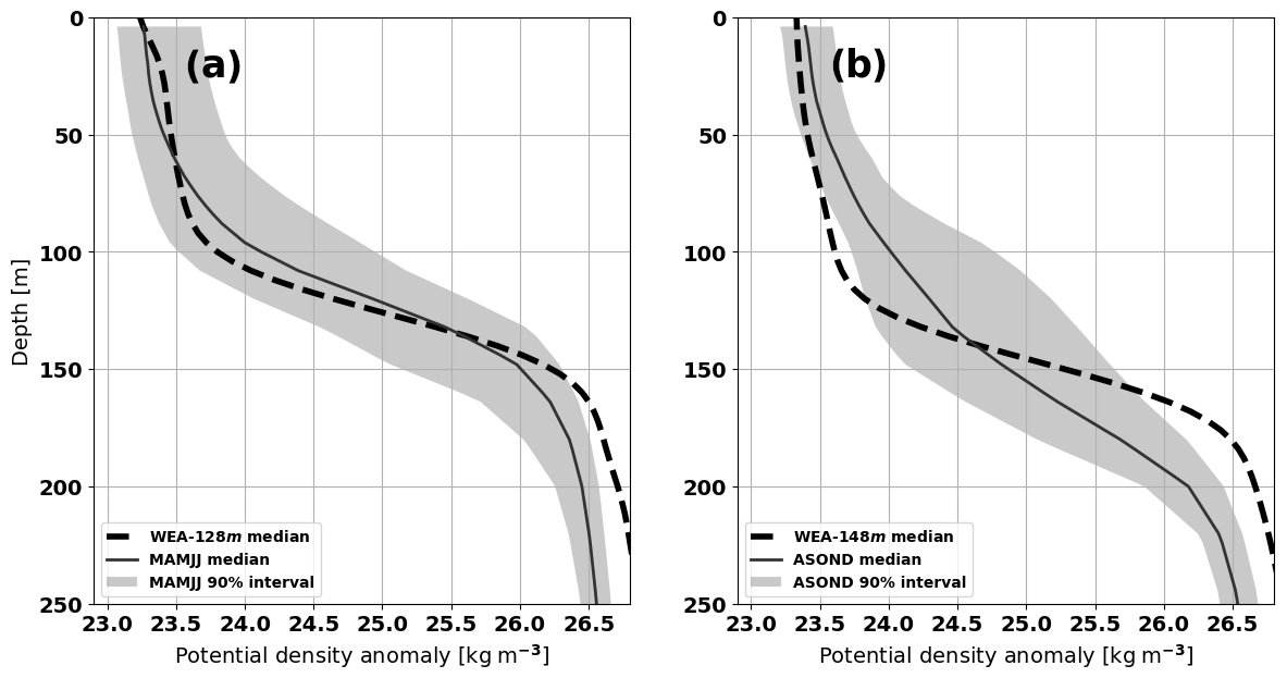
Figure C1Stratification in NEMO simulation at 46∘ W between 0 and 2∘ N for two seasons: (a) from March to July (MAMJJ) and (b) from August to December (ASOND). WEA refers to the classification developed in this present study. Data from Tchilibou et al. (2021).
The hydrodynamic code T-UGOm (CECILL licence) is available at https://hg.legos.obs-mip.fr/tugo (last access: 4 October 2021) (Mercurial repository, 2021). The climatology of IT properties in the Bay of Biscay is available upon request to the authors.
The supplement related to this article is available online at: https://doi.org/10.5194/os-17-1563-2021-supplement.
SB developed the clustering methodology, ran the simulations and realized all the graphics and interpretations. FL developed T-UGOm, built the model configuration for previous studies and supervised the runs. FL, MT and LC enhanced the interpretations and graphics with their relevant advice.
The authors declare that they have no conflict of interest.
Publisher's note: Copernicus Publications remains neutral with regard to jurisdictional claims in published maps and institutional affiliations.
The authors are grateful to the CNES, CLS, CNRS and UPS for the funding of this study as well as the projects COCTO (PIs: Nadia Ayoub and Pierre De Mey-Frémaux) and HighFreq (PI: Florent Lyard) for the additional funding of diverse missions for the communication of this study. Damien Allain is also thanked for his help with the simulations and the development of POCViP. The developers of the Scikit-learn Python package (Pedregosa et al., 2011) are thanked for providing a well-documented package on machine learning algorithms. Rosemary Morrow is thanked for her helpful comments on how to make the article easily understandable and on the writing of this article.
This study have been supported by CNES (grant no. 2884), CLS and CNRS (grant no. 167349).
This paper was edited by Ilker Fer and reviewed by three anonymous referees.
Barbot, S.: Internal tide realistic modeling: surface signature, variability and energy budget, PhD thesis, Université de Toulouse, Toulouse, accepted, 2021. a
Charraudeau, R. and Vandermeirsch, F.: Bay of Biscay's temperature and salinity climatology, Tech. rep., Ifremer [data set], available at: http://www.ifremer.fr/climatologie-gascogne/reference/summary_sea_tech_we.pdf (last access: 26 February 2021), 2006. a
Feistel, R.: A new extended Gibbs thermodynamic potential of seawater, Prog. Oceanogr., 58, 43–114, 2003. a
Feistel, R.: A Gibbs function for seawater thermodynamics for −6 to 80 ∘C and salinity up to 120 g kg−1, Deep-Sea Res. Pt. I, 55, 1639–1671, 2008. a
Ffield, A.: North Brazil current rings viewed by TRMM Microwave Imager SST and the influence of the Amazon Plume, Deep-Sea Res. Pt. I, 52, 137–160, 2005. a
Fu, L.-L. and Ubelmann, C.: On the transition from profile altimeter to swath altimeter for observing global ocean surface topography, J. Atmos. Ocean. Tech., 31, 560–568, 2014. a
Gaillard, F.: ISAS-13-CLIM temperature and salinity gridded climatology, SEANOE [data set], https://doi.org/10.17882/45946, 2015. a
Garraffo, Z. D., Johns, W. E., Chassignet, E. P., and Goni, G. J.: North Brazil Current rings and transport of southern waters in a high resolution numerical simulation of the North Atlantic, in: Elsevier Oceanography Series, vol. 68, Elsevier, Amsterdam, 375–409, 2003. a, b, c, d
Garzoli, S. L., Ffield, A., Johns, W. E., and Yao, Q.: North Brazil Current retroflection and transports, J. Geophys. Res., 109, C01013, https://doi.org/10.1029/2003JC001775, 2004. a
Goni, G. J. and Johns, W. E.: Synoptic study of warm rings in the North Brazil Current retroflection region using satellite altimetry, in: Elsevier Oceanography Series, vol. 68, Elsevier, 335–356, 2003. a, b
Gustafsson, F.: Determining the initial states in forward-backward filtering, IEEE T. Sig. Process., 44, 988–992, https://doi.org/10.1109/78.492552, 1996. a
Johns, W. E., Lee, T., Beardsley, R., Candela, J., Limeburner, R., and Castro, B.: Annual cycle and variability of the North Brazil Current, J. Phys. Oceanogr., 28, 103–128, 1998. a
Le Bars, Y., Lyard, F., Jeandel, C., and Dardengo, L.: The AMANDES tidal model for the Amazon estuary and shelf, Ocean Model., 31, 132–149, 2010. a
Lyard, F., Barbot, S., and Nugroho, D.: T-UGOm hydrodynamic model [code], in preparation, 2021b. a
Lyard, F. H., Allain, D. J., Cancet, M., Carrère, L., and Picot, N.: FES2014 global ocean tide atlas: design and performance, Ocean Sci., 17, 615–649, https://doi.org/10.5194/os-17-615-2021, 2021a. a, b
Magalhaes, J. M., da Silva, J. C. B., Buijsman, M. C., and Garcia, C. A. E.: Effect of the North Equatorial Counter Current on the generation and propagation of internal solitary waves off the Amazon shelf (SAR observations), Ocean Sci., 12, 243–255, https://doi.org/10.5194/os-12-243-2016, 2016. a
Marsaleix, P., Auclair, F., Floor, J. W., Herrmann, M. J., Estournel, C., Pairaud, I., and Ulses, C.: Energy conservation issues in sigma-coordinate free-surface ocean models, Ocean Model., 20, 61–89, 2008. a
Mercurial repository: https://hg.legos.obs-mip.fr/tugo, Mercurial repository [code], last access: 4 October 2021. a
Millero, F. J., Feistel, R., Wright, D. G., and McDougall, T. J.: The position of Standard Seawater and the definition of the Reference-Composition Salinity Scale, Deep-Sea Res. Pt. I, 55, 50–72, 2008. a
Morrow, R., Fu, L.-L., Ardhuin, F., Benkiran, M., Chapron, B., Cosme, E., d'Ovidio, F., Farrar, J. T., Gille, S. T., Lapeyre, G., Le Traon, P.-Y., Pascual, A., Ponte, A., Qiu, B., Rascle, N., Ubelmann, C., Wang, J., and Zaron, E. D.: Global observations of fine-scale ocean surface topography with the Surface Water and Ocean Topography (SWOT) mission, Front. Mar. Sci., 6, 232, https://doi.org/10.3389/fmars.2019.00232, 2019. a
Nugroho, D.: The tides in a general circulation model in the Indonesian seas, Ocean, Atmosphere, Université Paul Sabatier – Toulouse III, available at: https://tel.archives-ouvertes.fr/tel-01897523/document (last access: 1 October 2021), 2017. a, b, c
Pairaud, I. L., Auclair, F., Marsaleix, P., Lyard, F., and Pichon, A.: Dynamics of the semi-diurnal and quarter-diurnal internal tides in the Bay of Biscay. Part 2: Baroclinic tides, Cont. Shelf Res., 30, 253–269, 2010. a
Pedregosa, F., Varoquaux, G., Gramfort, A., Michel, V., Thirion, B., Grisel, O., Blondel, M., Prettenhofer, P., Weiss, R., Dubourg, V., Vanderplas, J., Passos, A., Cournapeau, D., Brucher, M., Perrot, M., and Duchesnay, E.: Scikit-learn: Machine Learning in Python, J. Mach. Learn. Res., 12, 2825–2830, 2011. a, b
Pichon, A. and Correard, S.: Internal tides modelling in the Bay of Biscay. Comparisons with observations, Scientia Marina, 70, 65–88, 2006. a
Pichon, A. and Maze, R.: Internal Tides over a Shelf Break: Analytical Model And Observations, American Meteorological Society, Boston, MA, USA, 657–671, https://doi.org/10.1175/1520-0485(1990)020<0657:ITOASB>2.0.CO;2, 1990. a
Piton, V., Herrmann, M., Lyard, F., Marsaleix, P., Duhaut, T., Allain, D., and Ouillon, S.: Sensitivity study on the main tidal constituents of the Gulf of Tonkin by using the frequency-domain tidal solver in T-UGOm, Geosci. Model Dev., 13, 1583–1607, https://doi.org/10.5194/gmd-13-1583-2020, 2020. a
Ray, R. D. and Mitchum, G. T.: Surface manifestation of internal tides generated near Hawaii, Geophys. Res. Lett., 23, 2101–2104, 1996. a
Ray, R. D. and Zaron, E. D.: M2 Internal Tides and Their Observed Wavenumber Spectra from Satellite Altimetry, J. Phys. Oceanogr., 46, 3–22, https://doi.org/10.1175/JPO-D-15-0065.1, 2016. a, b, c
Richardson, P. and Reverdin, G.: Seasonal cycle of velocity in the Atlantic North Equatorial Countercurrent as measured by surface drifters, current meters, and ship drifts, J. Geophys. Res.-Oceans, 92, 3691–3708, 1987. a
Ruault, V., Jouanno, J., Durand, F., Chanut, J., and Benshila, R.: Role of the tide on the structure of the Amazon plume: a numerical modeling approach, J. Geophys. Res.-Oceans, 125, e2019JC015495, https://doi.org/10.1029/2019JC015495, 2020. a, b, c
Soufflet, Y., Marchesiello, P., Lemarié, F., Jouanno, J., Capet, X., Debreu, L., and Benshila, R.: On effective resolution in ocean models, Ocean Model., 98, 36–50, 2016. a
Szekely, T., Gourrion, J., Pouliquen, S., and Reverdin, G.: CORA, Coriolis Ocean Dataset for Reanalysis, https://doi.org/10.17882/46219, 2016. a
Tchilibou, M., Gourdeau, L., Lyard, F., Morrow, R., Koch Larrouy, A., Allain, D., and Djath, B.: Internal tides in the Solomon Sea in contrasted ENSO conditions, Ocean Sci., 16, 615–635, https://doi.org/10.5194/os-16-615-2020, 2020. a, b, c
Tchilibou, M., Koch-Larrouy, A., Barbot, S., Lyard, F., Morel, Y., Jouanno, J., and Morrow, R.: Internal tides of the Amazon shelf during two contrasted seasons: Interactions with background circulation and SSH imprints, Ocean Sci., in preparation, 2021. a, b, c, d
Ward, J. J. H.: Hierarchical grouping to maximize payoff, Tech. rep., Personnel Research Lab, Lackland AFB, TX, 1961. a
Ward, J. J. H. and Hook, M. E.: Application of an hierarchical grouping procedure to a problem of grouping profiles, Educat. Psychol. Meas., 23, 69–81, 1963. a
Welch, P.: The use of fast Fourier transform for the estimation of power spectra: a method based on time averaging over short, modified periodograms, IEEE T. Audio Electroacoust., 15, 70–73, 1967. a
Zaron, E. D.: Baroclinic Tidal Sea Level from Exact-Repeat Mission Altimetry, J. Phys. Oceanogr., 49, 193–210, https://doi.org/10.1175/JPO-D-18-0127.1, 2019. a, b, c, d
Zaron, E. D. and Ray, R. D.: Using an altimeter-derived internal tide model to remove tides from in situ data, Geophys. Res. Lett., 44, 4241–4245, 2017. a, b, c, d
Zhao, Z., Wang, J., Fu, L.-L., Chen, S., Qiu, B., and Menemenlis, D.: Mapping Internal Tides using Synthetic SWOT Measurements, in: AGU Fall Meeting Abstracts, 10–14 December 2018, Washington, 2018. a
http://marine.copernicus.eu/, last access: 26 Febuary 2021.
https://www.seanoe.org/, last access: 26 Febuary 2021.
http://www.ifremer.fr/climatologie-gascogne/climatologie/index.php, last access: 26 February 2021.
https://github.com/TEOS-10/python-gsw, last access: 26 February 2021.
https://docs.scipy.org/doc/scipy/reference/signal.html, last access: 26 February 2021.
- Abstract
- Introduction
- The classification of the density profiles
- Sensitivity of the internal tides to the background stratification
- Conclusions
- Appendix A: western equatorial Atlantic additional visualization of the clusters
- Appendix B: Bathymetry used in the COMODO configuration
- Appendix C: Seasonal stratification of NEMO simulation
- Code and data availability
- Author contributions
- Competing interests
- Disclaimer
- Acknowledgements
- Financial support
- Review statement
- References
- Supplement