Lagrangian eddy tracking reveals the Eratosthenes anticyclonic attractor in the eastern Levantine Basin

Statistics of anticyclonic eddy activity and eddy trajectories in the Levantine Basin over the 2000–2018 period are analyzed using the DYNED-Atlas database, which links automated mesoscale eddy detection by the Angular Momentum Eddy Detection and Tracking Algorithm (AMEDA) algorithm to in situ oceanographic observations. This easternmost region of the Mediterranean Sea, delimited by the Levantine coast and Cyprus, has a complex eddying activity, which has not yet been fully characterized. In this paper, we use Lagrangian tracking to investigate the eddy fluxes and interactions between different subregions in this area. The anticyclonic structure above the Eratosthenes Seamount is identified as hosting an anticyclone attractor, constituted by a succession of long-lived anticyclones. It has a larger radius and is more persistent (staying in the same position for up to 4 years with successive merging events) than other eddies in this region. Quantification of anticyclone flux shows that anticyclones that drift towards the Eratosthenes Seamount are mainly formed along the Israeli coast or in a neighboring area west of the seamount. The southeastern Levantine area is isolated, with no anticyclone transfers to or from the western part of the basin, defining the effective attraction basin for the Eratosthenes anticyclone attractor. Co-localized in situ profiles inside eddies provide quantitative information on their subsurface physical anomaly signature, whose intensity can vary greatly with respect to the dynamical surface signature intensity. Despite interannual variability, the so-called Eratosthenes anticyclone attractor stores a larger amount of heat and salt than neighboring anticyclones, in a deeper subsurface anomaly that usually extends down to 500 m. This suggests that this attractor could concentrate heat and salt from this subbasin, which will impact the properties of intermediate water masses created there.

1 Introduction

The circulation in the eastern part of the Mediterranean Sea has not been investigated as extensively as the western part, and some aspects of its circulation are still the subject of scientific debate. Different pathways for the mean flow have been proposed with notable differences in the Gulf of Sidra and the Levantine Basin (LB) (Robinson et al., 1991; Hamad et al., 2006). Since the satellite sea surface temperature (SST) images in the 1990s, there has been overall agreement regarding the mean counterclockwise surface circulation in the eastern Mediterranean Basin, with the Atlantic waters (AWs) coming through the Strait of Sicily, following the Libyo-Egyptian coast, and then continuing along the Levantine and Turkish coasts (Hamad et al., 2006).

The Levantine Basin, defined as the part of the eastern Mediterranean, south of 37^∘ N and east of 23^∘ E (Hamad et al., 2006), appears to have a rather complex and turbulent circulation, particularly in its southeastern part, bound by the topography of Cyprus and the Egyptian and Levantine coasts. Extensive in situ oceanographic surveys have been performed in previous decades (Robinson et al., 1991; Brenner, 1993; Hayes et al., 2011); of note is the work of the Physical Oceanography of the Eastern Mediterranean (POEM) group, which detected some recurrent large long-lived (lasting longer than a year) anticyclonic structures in the 1980s: Ierapetra southeast of Crete and Marsa Matruh offshore of Egypt above the Herodotus Trench, at approximately 33.2^∘ N, 32.3^∘ E (see scheme from Robinson et al., 1991). South of Cyprus, different authors proposed a multipole structure named “Shikmona”, and they named the most active feature of this structure the “Cyprus eddy” (Brenner, 1993; Zodiatis et al., 2010). However, due to their limited time coverage, these studies had a static perspective. Zodiatis et al. (2010) probably presents the most advanced vision from this approach, displaying a hint of interannual variability. In the more recent hydrographic regionalization review of Ayata et al. (2018), the anticyclonic structure south of Cyprus is called the “Eratosthenes anticyclone”, which is the name used hereafter.

In the 1990s, the development of satellite observation, initially undertaken using SST, already enabled the identification of some of these long-lived anticyclonic structures as accumulation areas for mesoscale eddies detached from the coast (Millot and Taupier-Letage, 2005; Hamad et al., 2006). Later altimetry products of sea surface height (SSH) such as Archiving, Validation, and Interpretation of Satellite Oceanographic Data (AVISO)/Copernicus Marine Environment Monitoring Service (CMEMS) with a grid resolution on the order of the deformation radius helped to investigate the unsteady dynamics of mesoscale structures in the region. Although not detected in instantaneous views, a constant and strong AW flux also exists in the center of the eastern basin in a turbulent Mid-Mediterranean Jet (MMJ) (Amitai et al., 2010). However, studies such as Amitai et al. (2010) used sea level anomalies fields (SLAs) and an Eulerian approach of turbulence instead of focusing on individual eddy behavior. Thus, eddy climatology in the LB remains unknown, and impact on water masses transport performed by such transient eddies has not yet been studied. Figure 1 presents the topography of the LB, overlaid with mean dynamic topography (MDT) from 2000 to 2018 retrieved from CMEMS at a $\mathrm{1}/\mathrm{8}$^∘ resolution. The Eratosthenes Seamount, whose summit is about 700 m deep at approximately 33.7^∘ N, 32.7^∘ E, appears to be a prominent topographic feature in the basin and indeed displays a mean anticyclonic circulation with a closed contour of higher MDT, coherent with recent campaigns sampling the Eratosthenes anticyclone (previously named the “Cyprus eddy”) (Hayes et al., 2011; Moutin and Prieur, 2012). However, some differences from previous studies also appear, as this eddy is shifted westwards from its former reported location closer to the Levantine coast, at approximately 33.5^∘ N, 33.5^∘ E (Brenner, 1993; Amitai et al., 2010). Although there have been improvements in the SSH products since Amitai et al. (2010) (Taburet et al., 2019), this westward trend seems to be a physical displacement of the Eratosthenes anticyclone (Zodiatis et al., 2010).

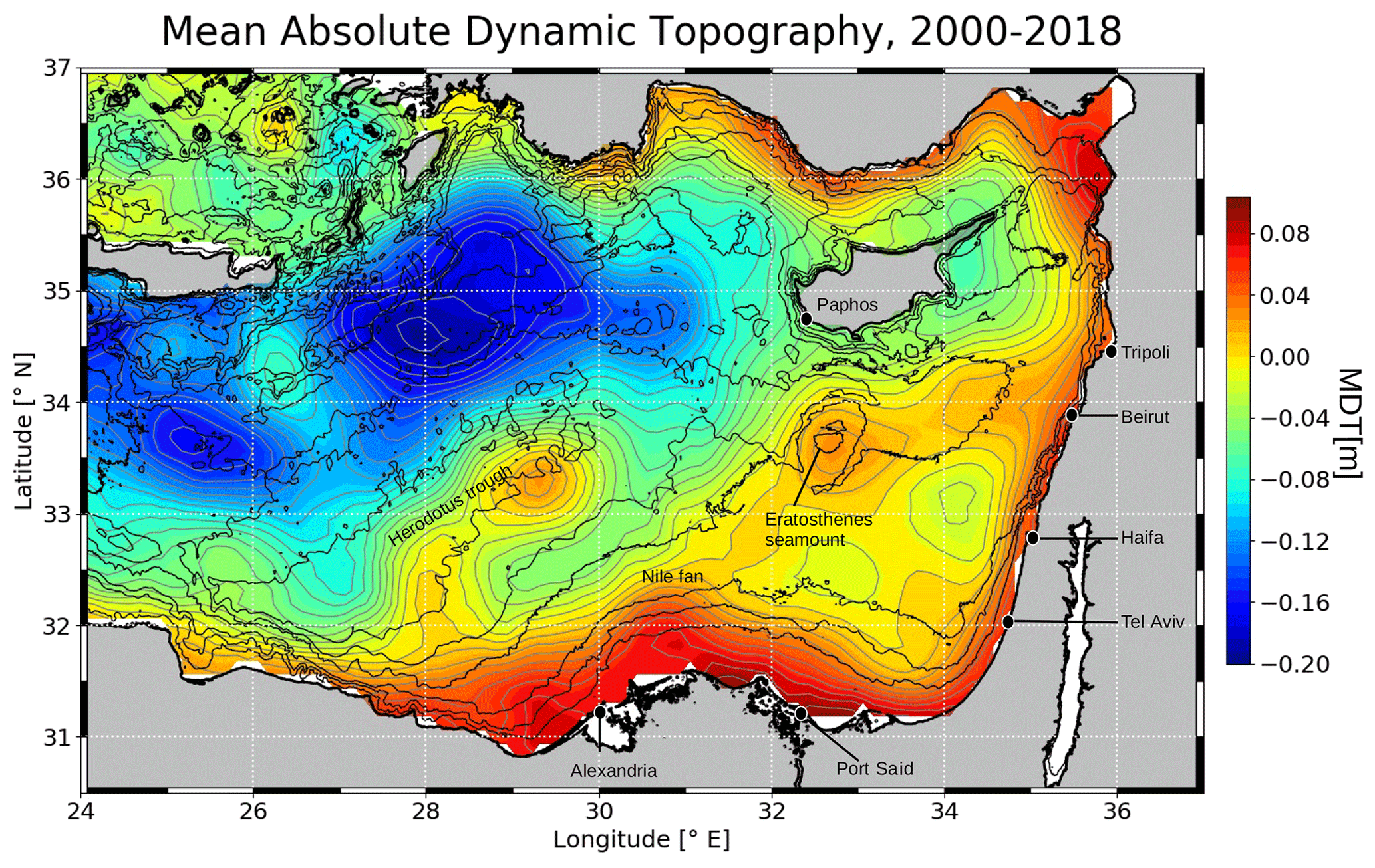
Figure 1 Mean dynamic topography (MDT) map of the LB and several toponyms used in this study. Thin black lines are the −100, −500, −1000, −1500, −2000 and −2500 m isobaths, and the thick black line is the 0 m isobath. Bathymetry is retrieved from GEBCO (2020). The same isobaths are shown on all maps.

Intense eddy activity in a basin with strong topographic constraints may lead to numerous eddy–eddy interactions, and highlights the need to take merging and splitting events between mesoscale structures into account. Initially, eddy automated detection and tracking algorithms were mostly based on SSH fields and did not detect such interactions (Chelton et al., 2011; Mason et al., 2014). Over the past decades, numerous algorithms have been further developed to take merging and splitting events into account, based on SSH (Matsuoka et al., 2016; Cui et al., 2019; Laxenaire et al., 2018) or a mixed velocity field–SSH approach (Yi et al., 2014; Le Vu et al., 2018).

The Angular Momentum Eddy Detection and Tracking Algorithm (AMEDA) developed by Le Vu et al. (2018) is used in this study. It detects eddy centers by computing the local normalized angular momentum (LNAM) introduced by Mkhinini et al. (2014) – as opposed to using the Okubo–Weiss parameter, as in Yi et al. (2014) – and computes the maximal tangential speed within the largest surrounding closed SSH contours to find eddy contours. Eddy observations at different time steps are gathered in tracks by minimizing a cost function, which considers the spatial proximity, as well as changes in eddy size and intensity. Merging and splitting events are next detected as the outcome of eddy interactions – when two eddies share a closed SSH contour with an averaged velocity higher than that for each eddy taken separately. The AMEDA algorithm has been used successfully in various case studies, notably in the Algerian Basin by Garreau et al. (2018) and in the Arabian Sea by de Marez et al. (2019). The detection of merging and splitting events enables one to reconstruct the eddy network, with mesoscale structures not being independent but often interacting with each other. Following this idea, Laxenaire et al. (2018) was able to show the connection between the Indian and Atlantic oceans through Agulhas rings crossing the Southern Atlantic. However, while several studies have developed algorithms to detect eddy interactions, we are not aware of any studies that have quantified or analyzed the additional information from merging and splitting events in terms of eddy behavior, apart from Laxenaire et al. (2018).

Nevertheless, satellite analysis alone cannot reveal the subsurface structure. Moutin and Prieur (2012), for instance, studied three anticyclones in the Mediterranean Sea with similar SLA signatures but discovered extremely different heat and salt integrated anomalies. In the LB, Gertman et al. (2010) discovered smaller-scale eddies detaching from the Israeli coast through SST and drifters data, and Hayes et al. (2011) discovered a huge salt anomaly in the Eratosthenes anticyclone despite a weak SSH signature. These studies show the importance of in situ observations in addition to satellite data, but they were campaign-specific instantaneous observations. Before eddy automated detection, Menna et al. (2012) conducted a statistical study of mesoscale interactions in the LB by adding in situ drifter velocities to SSH-derived velocities, but sampling was sparse and without vertical information. The large-scale deployment of autonomous drifters in the global ocean (such as the Argo or MEOP programs), as well as the centralization of collected data (such as CMEMS products), enables one to bridge the gap in the temporal scale between satellite and in situ data. Argo is a global array of more than 3000 floats measuring temperature and salinity down to 2000 m (ARGO, 2020). Using Argo data, Laxenaire et al. (2019) captured the subsurface evolution of one single Agulhas ring over 1.5 years in the South Atlantic with the conjunction of Argo profiles and SSH data. This demonstrates that long-lived anticyclones can transport warm water masses over very long distances isolated in their thick core. Recently, in the Algerian Basin, Pessini et al. (2018) attempted to link eddy observations to in situ measurements and to compute eddy regional statistics, although they utilized an algorithm that did account for merging and splitting events. Mason et al. (2019) also attempted to study the vertical eddy structure with regional variation in the Alboran Sea, although they used data from assimilated models. Thus far, no such regional characterization of eddy systematic detection has been attempted in the eastern Mediterranean.

This approach of both eddy tracking, detected by altimetry that takes merging and splitting events into account, and co-localization with in situ observations can be generalized into an eddy atlas. The DYNED-Atlas database combines over 19 years of subsurface observations from Argo floats of identified eddies, tracked in time and space by the AMEDA algorithm (DYNED-Atlas-Med, 2019). The DYNED-Atlas is the perfect tool for the study of eddy dynamics and the associated transport of water masses in their cores, as it combines eddy detection and physical properties. It has not been exploited in the LB yet, although Stegner et al. (2019) already demonstrated very deep subsurface eddy signatures in this area.

Using eddy contours, tracks and co-localized profiles from the DYNED-Atlas database, extended with available expendable bathythermograph (XBT) and conductivity–temperature–density (CTD) profiles to compensate for the sparsity of observations, this study will investigate additional information from Lagrangian anticyclone tracking and statistically significant drift patterns and structures in the southeastern LB – east of 28^∘ E and south of Cyprus. After introducing the datasets in Sect. 2, we present our methodology of a Lagrangian convergence framework and the regions studied in Sect. 3. Analysis of this method with DYNED-Atlas data is detailed in Sect. 4. Vertical structure oceanographic observations co-localized inside eddies are used to study the eddy vertical signatures (Sect. 5). Possible mechanisms at work and hydrographic effects are discussed in Sect. 6.

2 Data

2.1 Eddy contours, centers and tracks

The dynamical evolution of eddies and their individual tracks are retrieved from the DYNED-Atlas database (DYNED-Atlas-Med, 2019) for the 2000–2018 period. The DYNED-Atlas project, with eddy tracks and physical property signatures, is accessible online: https://www1.lmd.polytechnique.fr/dyned/ (last access: 18 August 2021). The dynamical characteristics of the eddies contained in the DYNED-Atlas database were computed by the AMEDA eddy detection algorithm (Le Vu et al., 2018) applied on daily surface velocity fields. The latter were derived from the absolute dynamic topography (ADT) maps produced by Salto/Duacs and distributed by the Copernicus Marine Environment Monitoring Service (CMEMS) with a spatial resolution of $\mathrm{1}/\mathrm{8}$^∘, which is on the order of the internal deformation radius in the Mediterranean Sea (10–12 km; Mkhinini et al., 2014). A cyclostrophic correction is applied on these geostrophic velocities to accurately quantify eddy dynamical properties (Ioannou et al., 2019). Unlike standard eddy detection and tracking algorithms, the main advantage of the AMEDA algorithm is that it detects the merging and the splitting events (Le Vu et al., 2018), which allows one to build a network of trajectories associated with each eddy. In other words, we can reconstruct the eddy's “genealogy”.

2.2 Remote sensing measurements

To compute the MDT over the 2000–2018 period, we use the daily high-resolution ($\mathrm{1}/\mathrm{8}$^∘) AVISO ADT delayed-time product provided by CMEMS (SEALEVEL_MED_PHY_L4_REP_OBSERVATIONS_008_051). This altimetry gridded product is also used to locate the in situ CTD or glider measurements associated with the characteristic eddy contours in Sect. 5. Otherwise, to more precisely confirm the location of eddies and their size on specific days, we use the high-resolution ($\mathrm{1}/\mathrm{120}$^∘) merged-multisensor SST data representative of nighttime values provided by CMEMS (SST_MED_SST_L3S_NRT_OBSERVATIONS_010_012).

2.3 In situ oceanographic observations

About 34 406 Argo profiles are available from the DYNED-Atlas database in the whole Mediterranean Sea over this 19-year period. However, due to sparser campaigns, only 9384 were available in the LB, mostly after 2014. To complete these in situ measurements, we added 2311 CTD and 3860 XBT casts downloaded from the SeaDataNet portal (https://www.seadatanet.org/Data-Access, last access: 15 June 2020, data in unrestricted access) as well as 7020 additional profiles from the CORA (Coriolis Ocean database ReAnalysis) database, which is also available on the CMEMS catalogue: INSITU_GLO_TS_REP_OBSERVATIONS_013_001_b (https://resources.marine.copernicus.eu/?option=com_csw&view=details&product_id=INSITU_GLO_TS_REP_OBSERVATIONS_013_001_b, last access: 15 June 2020). Finally, glider measurements carried out in October 2018 by the Israel Oceanographic and Limnological Research (IOLR) in one transect offshore of Israel provided 370 profiles that were added to the database. The data sources listed above add up to 22 945 profiles from 2000 to 2018 in the LB. All of the hydrological profiles are then co-localized with detected eddies following the standard procedure used in the DYNED-Atlas database. Profiles are considered to be inside an eddy if they are inside its maximal speed contour.

3 Methodology

As opposed to previous studies that either considered eddy activity from “building-block” structures (Robinson et al., 1991) or eddy kinetic energy (EKE) fields derived from SLA compared to a MDT (Amitai et al., 2010), we follow eddies as daily, individual detections gathered in tracks. Eddies are not only active as individuals but also as a network of turbulent structures interacting with each other. Hence, the importance of taking merging and splitting events into account to reconstruct this network. This approach then aims to quantify eddy transfers between different subregions. This is similar to and greatly inspired by the previous work done by Laxenaire et al. (2018) for Agulhas rings in the South Atlantic.

3.1 Lagrangian convergence framework

Here, we define a framework to count eddy transfers imported to and exported from a study region, whose successive steps are shown in Fig. 2. The Eratosthenes Seamount region, studied as an example in Fig. 2, is bordered by a green line (coordinates in Table A1).

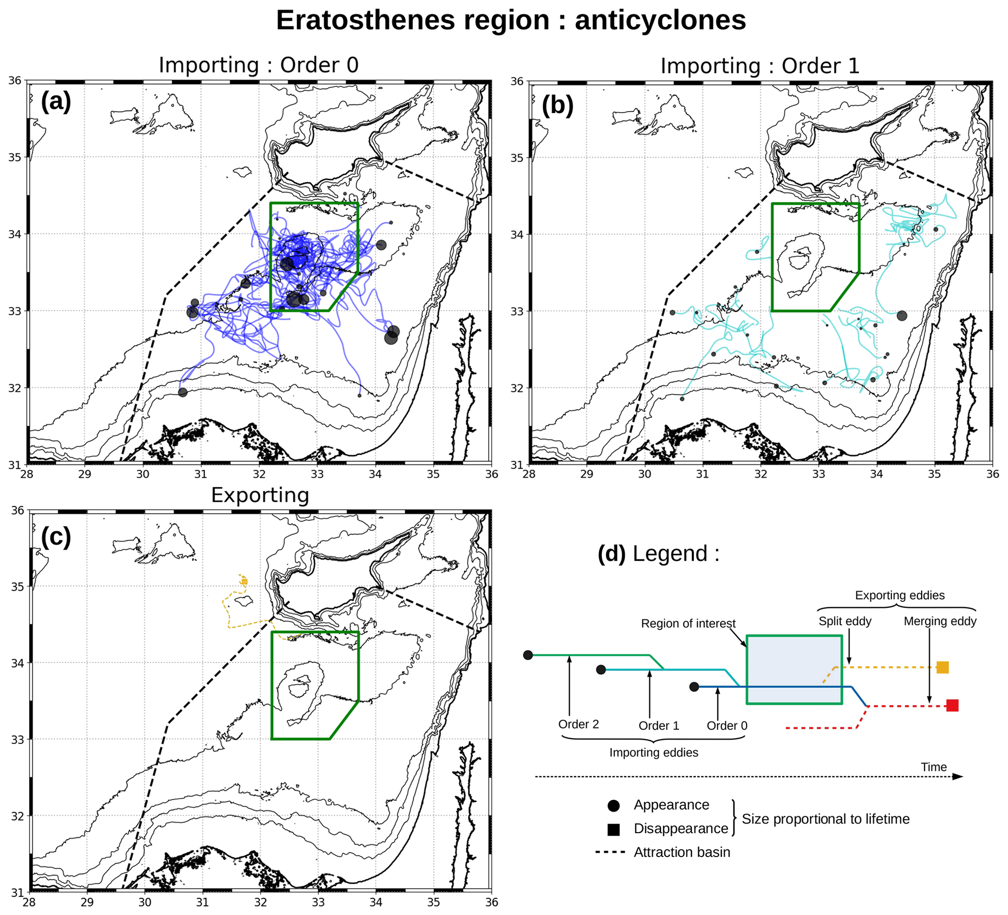
Figure 2 Lagrangian convergence framework applied to anticyclones in the Eratosthenes Seamount region and detailed in several steps: (a) order 0 – eddies converging directly; (b) order 1 – eddies merging with an order 0 eddy; (c) exporting split and merging eddies (no cases of the latter detected here). Locations of eddy appearance  (a, b) and eddy disappearance (c) are shown using black dots and colored squares, respectively, the size of which is proportional to the eddy lifetime. (d) The black dashed line is the attraction basin introduced in Sect. 4.3.

We consider importing eddies to be the eddies that are part of the family tree coming into a region. The order 0 eddies are defined as those converging directly to the region (the trajectories shown using blue lines in Fig. 2a). This order 0 label mainly encompasses eddies dying within the study region; however, some eddies can remain stationary for a very long period in the same area, later moving and dying in another place. In order to take the latter into account, the definition of an order 0 eddy is an eddy dying or spending more than half of its lifetime inside the perimeter of the study region. The sensitivity of this 50 % lifetime criterion is detailed in Fig. A1 in the Appendix, and this definition does not lead to inaccurately counting eddies that are just transiting the region as importing eddies. Indeed, eddies labeled as order 0 always disappear from the immediate vicinity when leaving the study region (see Fig. A2 for an example). Next, we label the eddies that merge with an order 0 eddy as order 1 (Fig. 2b, cyan lines). Recursively, we label the eddies that merge with an order 1 eddy as order 2 (not shown in Fig. 2 but displayed in Fig. 6a). Hereafter, we will discard orders higher than 2 from the discussion, as their quantity was found to be negligible.

In contrast, an exporting eddy flux moves some eddies outside of the region. We distinguish two categories of exporting eddies: (1) if two eddies undergo a splitting event and one of the split eddies spends more than half of its lifetime outside the region, it is considered an exporting split eddy; (2) if an order 0 eddy dies while merging with external eddies which themselves drift away from the region, this external eddy is considered an exporting merging eddy. Exporting split (yellow dashed lines) and merging (red dashed lines) eddies are shown in the example in Fig. 2c; however, none of the latter were detected for this particular region.

It should be noted that, in this framework, the order 0 label prevails over other labels defined: if an eddy meets the criteria for both order 0 and order 1, it is labeled as order 0 only. Additionally, exporting (split and merging) eddies are labeled as such only if they are not already labeled as an importing eddy. It should also be noted that eddies labeled as order 0 can be born within or outside of the given region. Lastly, a label is relative to a region: an eddy spending more than half of its lifetime in a region but drifting and dying in another is labeled as importing order 0 for both regions (see the discussion about Table A2 in Sect. 4.2). In this framework and in the figures hereafter, importing eddies are plotted at their appearance location using black dots with sizes proportional to the eddy lifetime to show the origin of the water masses. Exporting split and merging eddies are plotted at their disappearance location as squares, also scaled according to their lifetime. Trajectories are smoothed through a (10 km × 10 km) window. The color chart is summarized in Fig. 2d and used throughout this study.

Finally, attractiveness of a region with respect to eddies – for a given polarity – is estimated in the “net eddy gain”. This is the total number of importing eddies – the sum of orders 0–1–2 and possibly higher – minus the number of eddies already born in the region of interest. This gain is later shown in Table A2 and discussed in Sect. 4.2.

3.2 Definition of anticyclonic and cyclonic regions

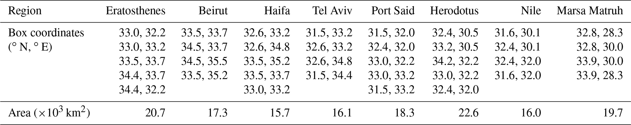
To further study the exchanges between eddying structures in the southeastern part of the LB, eight regions of interest are considered and shown in the MDT in Fig. 3. These regions are defined as closely as possible to nonoverlapping rectangular shapes, tiling as much of the southeastern corner of the LB as possible (≈78 % of the attraction basin discussed in Sect. 4.3 is covered) and with a similar size (areas and coordinates provided in Table A1 in the Appendix). Each box is defined to correspond to a structure in the MDT. Average cyclonic or anticyclonic activity can be inferred if it encompasses a depression or a hill in the MDT, respectively; hereafter, we refer to these regions as cyclonic (CY) or anticyclonic (AC) regions, respectively: Beirut (AC), Haifa (CY), Tel Aviv (AC), Port Said (CY), Herodotus (AC), Nile (AC) and Eratosthenes (AC, already shown in Fig. 2). Although not in our focus region, a comparison focused on the “Marsa Matruh” (AC) region is also carried out in Sect. 4.5. The eight distinct regions are presented on Fig. 3 with red or green solid borders denoting CY or AC regions, respectively. The attraction basin of the Eratosthenes region (see Sect. 4.3) is shown with a dashed line.

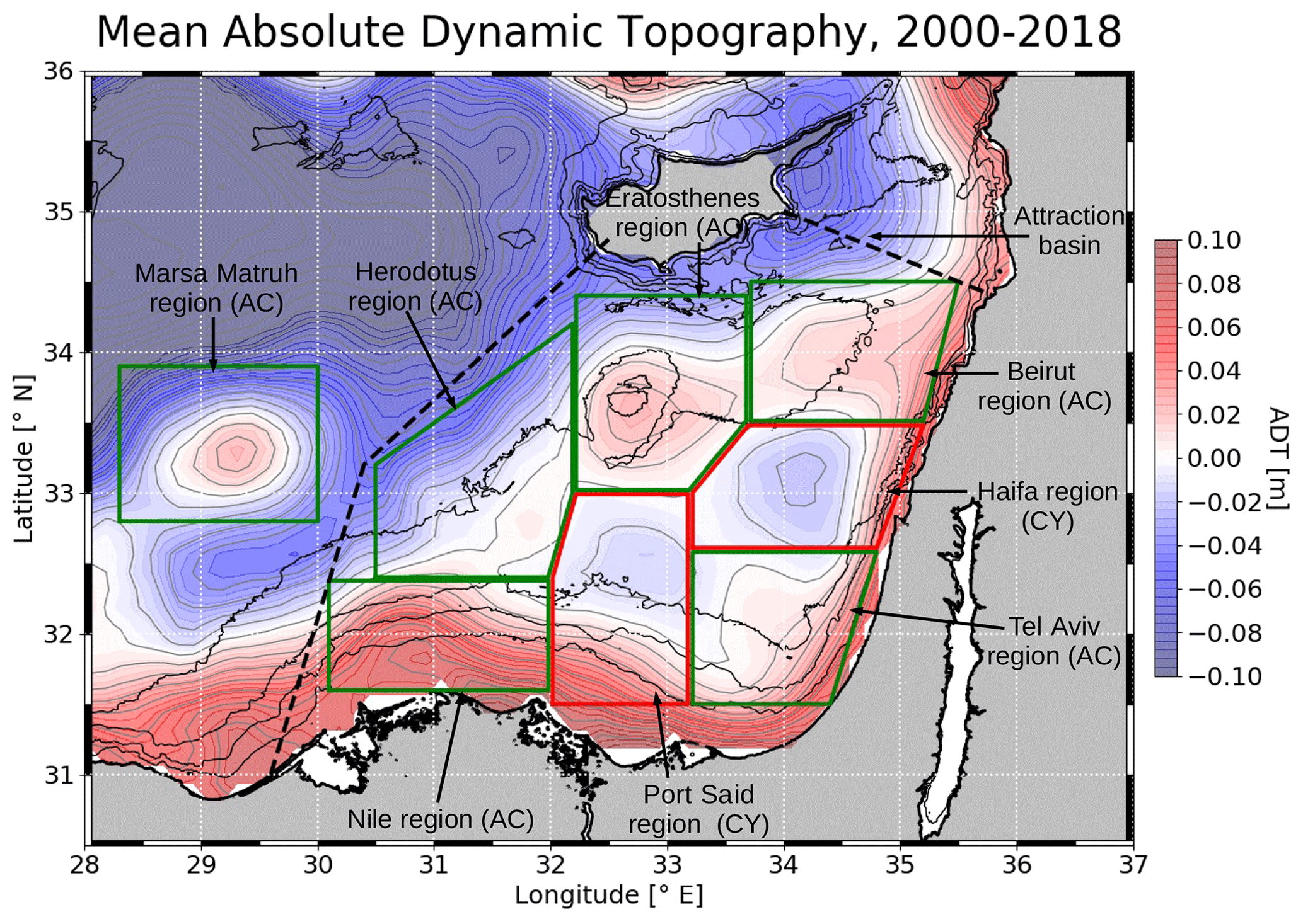
Figure 3 Mean dynamic topography (MDT) map of the southeastern LB labeled with borders and names of the study regions. Anticyclonic regions (AC) have a green border, cyclonic regions (CY) have a red border, and boxes are based on the coordinates indicated in the Appendix (Table A1). The black dashed line is the attraction basin introduced in Sect. 4.3.

3.3 Eddy-induced physical property anomalies

The DYNED-Atlas database establishes a method to estimate the physical property anomalies induced by an eddy (DYNED-Atlas-Med, 2019). This method is followed in this study, only extending the database with profiles from sources other than Argo and using in situ temperature instead of potential temperature to match up with XBT profiles. Each oceanographic measurement is compared to the AMEDA observations. If it falls within the contour of an eddy on the same day that it is cast, the profile is co-localized with the eddy and then considered as sampling its physical properties. If it falls outside any eddy observation, it is considered an “outside-eddy” profile. Estimation of the eddy-induced physical property anomalies (temperature, salinity, density) is next done by comparison with a reference background. For each observation, a climatological background is then computed by averaging all outside-eddy profiles from 2000 to 2018, at a distance smaller than 150 km from the its cast position and in the same season (in any year, but within a ±30 d period from the day of the cast). It is intended to be more statistically significant than estimates performed during a single campaign, usually through one profile inside an eddy and another one outside (e.g., Moutin and Prieur, 2012).

4 Lagrangian tracking results

4.1 Eddy activity from a Lagrangian framework

Figure 4 presents eddy occurrence and drift in the LB for anticyclones and cyclones, with the designated regions from Fig. 3. Time occurrence percentage (shown using color) is computed as the time spent inside the maximal speed contour of a detected eddy, whereas the drift (shown with arrows) is the mean speed of eddy centers passing through the pixel. The pixel size is $\mathrm{1}/\mathrm{8}$^∘ × $\mathrm{1}/\mathrm{8}$^∘. Gaussian smoothing is performed using a 5 pixel × 5 pixel kernel size, and data from pixels crossed by less than five eddy centers are discarded. This picture can be seen as an eddy Lagrangian approach equivalent to the MDT shown in Figs. 1 and 3, adding new information. Firstly, the spatial distribution of cyclonic and anticyclonic eddies is extremely inhomogeneous: almost no anticyclones are present in the northern part of the LB. The prevalence of the Marsa Matruh and Eratosthenes structures as persistent anticyclones is confirmed, with coherent spots hosting anticyclones for more than 50 % of the 2000–2018 time period. Cyclones are present in the southeastern part of the LB, in particular in the Haifa region. All anticyclonic (cyclonic) regions have on average a higher presence of anticyclones (cyclones), confirming (through a Lagrangian approach) the regions defined in Sect. 3.2. The comparison with the Ierapetra eddies southeast of Crete in Fig. 4 highlights the difference between Lagrangian and Eulerian visions. The Ierapetra eddies show up very clearly in SLA maps and are the most intense eddies in the region (Amitai et al., 2010). However, as they do not have fixed stable position and can drift far away after their formation (Ioannou et al., 2017), they form a less concentrated spot in Fig. 4. The Lagrangian vision then shows more persistent, although maybe less intense, structures.

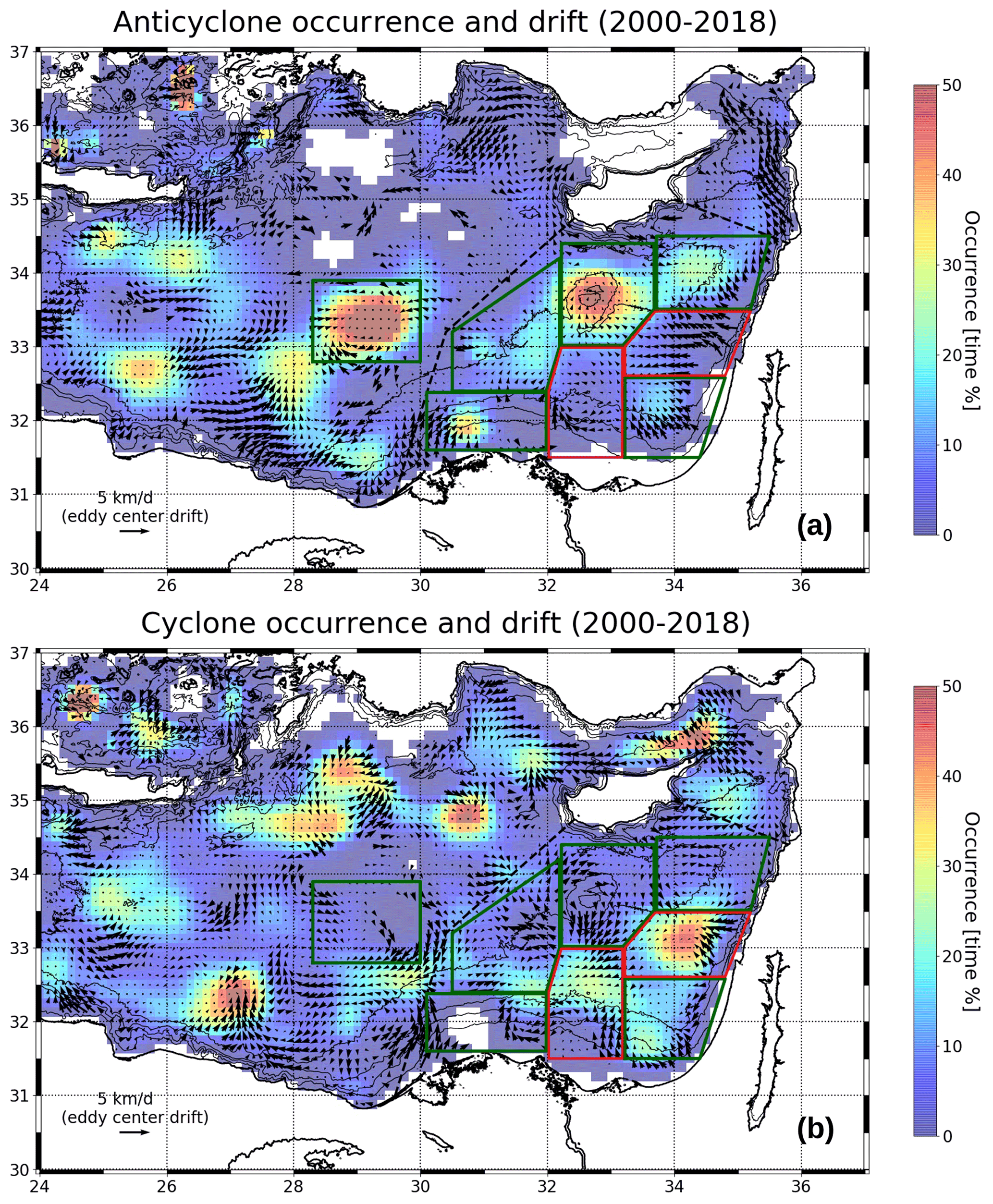
Figure 4 Eddy occurrence and drift in the LB for (a) anticyclones and (b) cyclones. The pixel size is $\mathrm{1}/\mathrm{8}$^∘ × $\mathrm{1}/\mathrm{8}$^∘. Occurrence is shown as the time percentage that the pixel center spends inside maximal speed contours of eddies. Eddy drift is the mean Lagrangian drift of the eddy centers on pixels that more than five eddy centers passed; Gaussian smoothing is carried out with a 5×5 kernel size. The AC (CY) regions defined in Sect. 3.2 are drawn using a green (red) solid line, and the attraction basin defined in Sect. 4.3 is drawn using a black dashed line.

Additionally, Fig. 5 shows eddy lifetime statistics in the LB, with a comparison of the normalized cumulative eddy lifetime (i.e., the probability for an eddy to live longer than a given time period). In the Mediterranean Sea, the lifetime for cyclones is on average far shorter than for anticyclones, as already shown by Mkhinini et al. (2014). However, this disequilibrium is even more pronounced in the LB: the cyclones lifetime distribution is very similar to the rest of the Mediterranean, whereas anticyclones clearly tend to live longer. As an example, in absolute units of detected eddies, 105 anticyclones (out of 5770) compared with 70 cyclones (out of 7159) are found to live longer than 400 d in the whole Mediterranean, whereas in the LB, 39 anticyclones (out of 1210) compared with 17 cyclones (out of 1630) live longer than 400 d. The intense Ierapetra anticyclones have been shown to often live more than 3 years (Ioannou et al., 2017); however, as no more than one of these eddies is formed each year, they can not explain the trend of longer anticyclone lifetimes. These statistics suggest the existence of mechanisms prolonging anticyclone lifetimes in the LB. Hence, this study specifically focuses on anticyclones, whose longer lifetimes also lead them to capture water masses in their core for an extended period and have higher hydrologic impact.

Figure 5 Cumulative eddy lifetime as a percentage on a logarithmic scale, separated for cyclones and anticyclones and for the LB and the whole Mediterranean Sea.

4.2 Inter-region anticyclone transfers

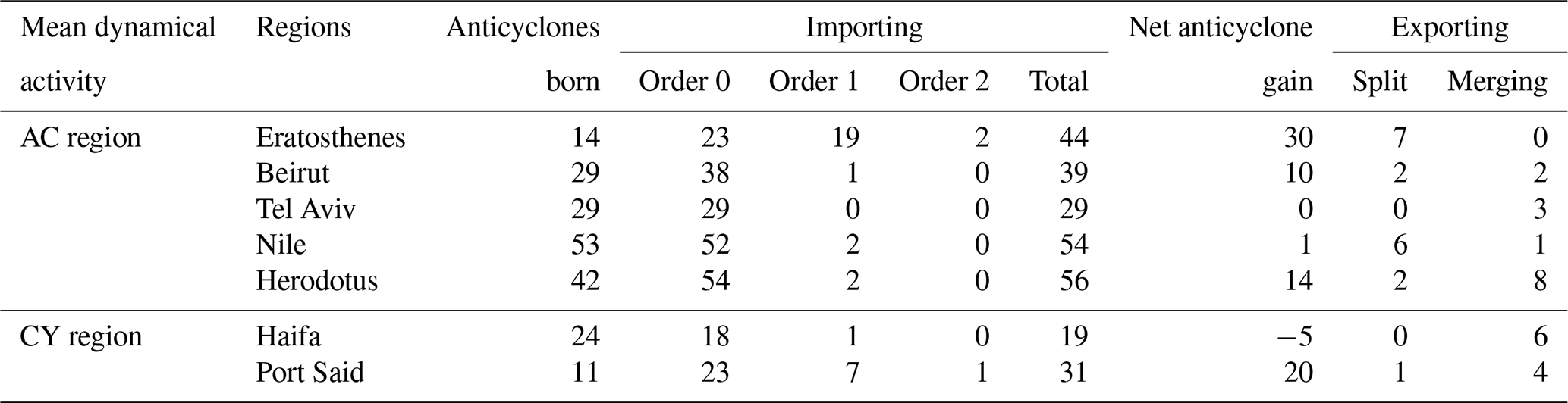
The Lagrangian convergence framework detailed in Sect. 3.1 is applied to the seven regions of the southeastern LB (Eratosthenes, Beirut, Haifa, Tel Aviv, Port Said, Herodotus and Nile, with Marsa Matruh being studied later in Sect. 4.5) in Fig. 6, only considering anticyclones (statistics also shown in Table A2). The color code is the same as in Fig. 2 and Fig. 6h. For each panel in Fig. 6, all other regions are shown, with green (red) borders for AC (CY) regions. The region to which each panel title refers is outlined using a thicker line. For all AC regions (Fig. 6a, b, d, f, g), anticyclones trajectories form a rather concentrated bulk at the center of the region, whereas CY regions (Fig. 6c, e) only have a very sparse and random anticyclone occurrence. The mean dynamical activity from Sect. 3.2 is confirmed, as only AC regions host a preference spot for anticyclones, whereas CY regions tend to be avoided by anticyclones.

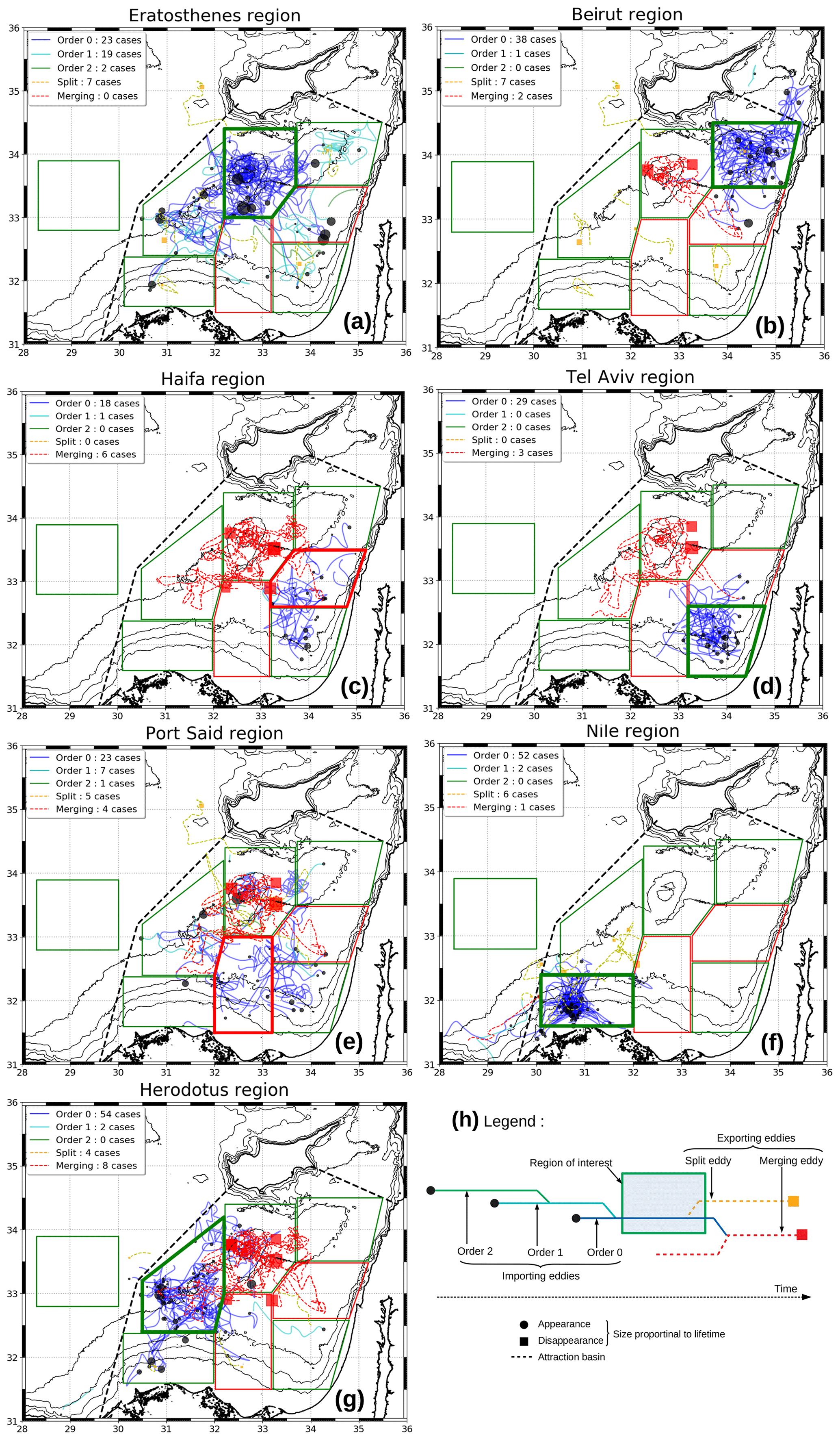
Figure 6 Eddy exchanges framework applied to the (a) Eratosthenes, (b) Beirut, (c) Haifa, (d) Tel Aviv, (e) Port Said, (f) Nile and (g) Herodotus regions. For each panel, all other regions are shown (green borders for AC regions, and red borders for CY regions); the thicker line indicates the study region. The color chart used is summarized in panel (h). The Marsa Matruh region is studied later in Fig. 10.

Important differences can, however, be noted between AC regions. In the Beirut region, anticyclones meander a lot but have few interactions (only two merging events and two splitting events in 19 years) and eddies have a moderate lifetime (126 d). In the Tel Aviv region, anticyclones are more short-lived (97 d on average), spend less time in the region with few meanders and four merging exports were recorded for the benefit of the Eratosthenes region; this characterizes the Tel Aviv region as an anticyclone formation region. Characterizing the Herodotus region is more difficult, as some eddies stem from the Nile region and some others eventually merge with Eratosthenes region long-lived anticyclones; thus, the Herodotus region seems to act as an anticyclone formation region (42 anticyclones born there) but also as a transitory region with respect to the Eratosthenes zone, with which it interacts a lot (eight merging exports). On the contrary, the Nile region is a strong and preferred anticyclonic spot, but eddies there interact very little with neighboring regions; the Nile region rather acts as a termination region for anticyclones formed to the west and following the Libyo-Egyptian coast.

Nonetheless, some anticyclones are formed inside CY regions, notably in the Haifa region. In this region anticyclones are generally short-lived (average lifetime of 94 d) and often disappear while being exported to the Eratosthenes region (six merging events recorded); the role of the Haifa region is then similar to the Tel Aviv region, acting as a region of anticyclone formation. The case of the Port Said region is more ambiguous, with no clear pattern being visible. Statistics in the Appendix (Table A2) seem to show that it attracts some anticyclones, but this can be due to the fact that some long-lived eddies of the Eratosthenes region sometimes venture approximately 100 km farther south. This ambiguity also shows the limits of this Lagrangian approach, as it is sensitive to a singular event for eddies with lifetimes longer than 3 years. As a comparison, Fig. A3 shows the same analysis as Fig. 6b for the Haifa region but studying cyclone transfers. Patterns for cyclones are less clear than for anticyclones, likely because cyclones have shorter lifetimes and are, thus, more numerous. However, it confirmed the Haifa region as a stable spot for cyclones.

4.3 Eratosthenes anticyclone attractor (EAA)

Figure 7 and Table A2 summarize anticyclone transfers in the southeastern LB. The attractiveness of each region is measured through the net eddy gain introduced in Sect. 3.1. The arrows in Fig. 7 indicate eddy transfers, with the thickness being proportional to the number of eddies transferred. The particular case of the Eratosthenes region shows a clear convergence with 44 importing anticyclones attracted, whereas only 14 were initially born in the region surrounding the Eratosthenes Seamount, from 2000 to 2018; this results in a net eddy gain of +30 and an approximate anticyclone flux of more than one merging per year. Instead of freely drifting westwards as expected from the β-drift (Chelton et al., 2011), anticyclone tracks shown in Fig. 2b (or alternatively Fig. 6a) reveal that eddies meander a lot over the high bathymetry, as shown by the density of blue tracks, seemingly trapped by the seamount. On the other hand, few exporting split eddies escape, and not a single exporting merging eddy is detected; these split eddies are even more short-lived, as shown by the small size of the disappearance square (Fig. 2c). This trend of a high net eddy gain along with few exporting eddies and the persistent anticyclonic activity in the Eratosthenes region (Fig. 4) allows for the identification of this region as hosting an anticyclonic attractor, which is hereafter referred to as the “Eratosthenes anticyclone attractor” (EAA).

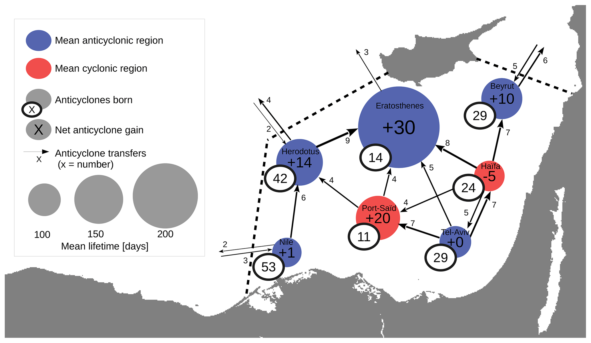
Figure 7 Scheme summarizing inter-region anticyclone transfers within the Eratosthenes anticyclone attractor (EAA) attraction basin (dashed line). Transfers encompass order 0–1–2 anticyclones. Within this basin, only transfers higher than or equal to 4 are represented by arrows (for legibility). All transfers across the basin border are shown. The arrow thickness is proportional to eddy transfers. Red circles represent CY regions, and blue circles represent AC regions; radii are proportional to the anticyclone mean lifetime in the region. More details are given in Table A2.

Moreover, this observed convergence toward the Eratosthenes Seamount seems to be geographically bound, with the tracks in Fig. 2a–b showing that anticyclones come from as far as 300 km away but with a distinct westward limit, depicted by a black dashed line. This area of anticyclones converging to the EAA, although constrained by topography, covers a large part of the southeastern LB and is called the EAA attraction basin in this study (see Figs. 3, 4, 6 and 7). It is defined as a straight line ranging from the Egyptian city of Alexandria (31.0^∘ N, 29.6^∘ E) to the Cypriot city of Paphos (34.8^∘ N, 30.4^∘ E) with a break angle at 33.2^∘ N, 30.4^∘ E and a second line closing it between the Greek cape on Cyprus island (35.0^∘ N, 34.1^∘ E) and the Lebanese city of Tripoli (34.4^∘ N, 35.8^∘ E).

Finally, Fig. 8 analyses the anticyclones constituting the EAA (i.e., order 0 importing anticyclones for the Eratosthenes region, shown using blue lines in Fig. 6a). The upper panel of Fig. 8 presents their time series, with the color indicating when the center is inside or outside of the region. An anticyclone is always present inside the region, with relay between long-lived eddies: each time an anticyclone inside the region dies, it is replaced by another, leading to only about 1 year out of 19 without an anticyclone over the Eratosthenes Seamount. Anticyclones in the Eratosthenes region also tend to be very different from their neighbors. Figure 8b classifies anticyclones in terms of mean maximal speed radius as a function of lifetime; each dot is an anticyclone labeled as order 0 for the seven regions studied in Fig. 6, with red color highlighting Eratosthenes anticyclones. The background is a density probability plot for all anticyclones in the LB – except Eratosthenes anticyclones to enhance comparison. The scatterplot presents an overall spread, with maximal density between 15 and 25 km, consistent with the limit of altimetric resolution ($\mathrm{1}/\mathrm{8}$^∘). However, long-lived Eratosthenes anticyclones form a clear cluster of eddies living longer than a year with a radius often greater than 40 km, outside the 90 % probability contour. Not all Eratosthenes anticyclones are encompassed in this category because the order 0 label also encompasses some short-lived eddies quickly merging, which unlikely have unusual characteristics – hence some of the red dots also being scattered. Eratosthenes anticyclones are the only eddies in the southeastern part of the LB that present such dynamical characteristics: apart from two outliers, this is the only region where the maximal speed radius can exceed 40 km, more than 3 times the internal deformation radius of approximately 10–12 km in the Mediterranean Sea (Mkhinini et al., 2014). This suggests the existence of different mechanisms acting on the eddy lifetime and radius.

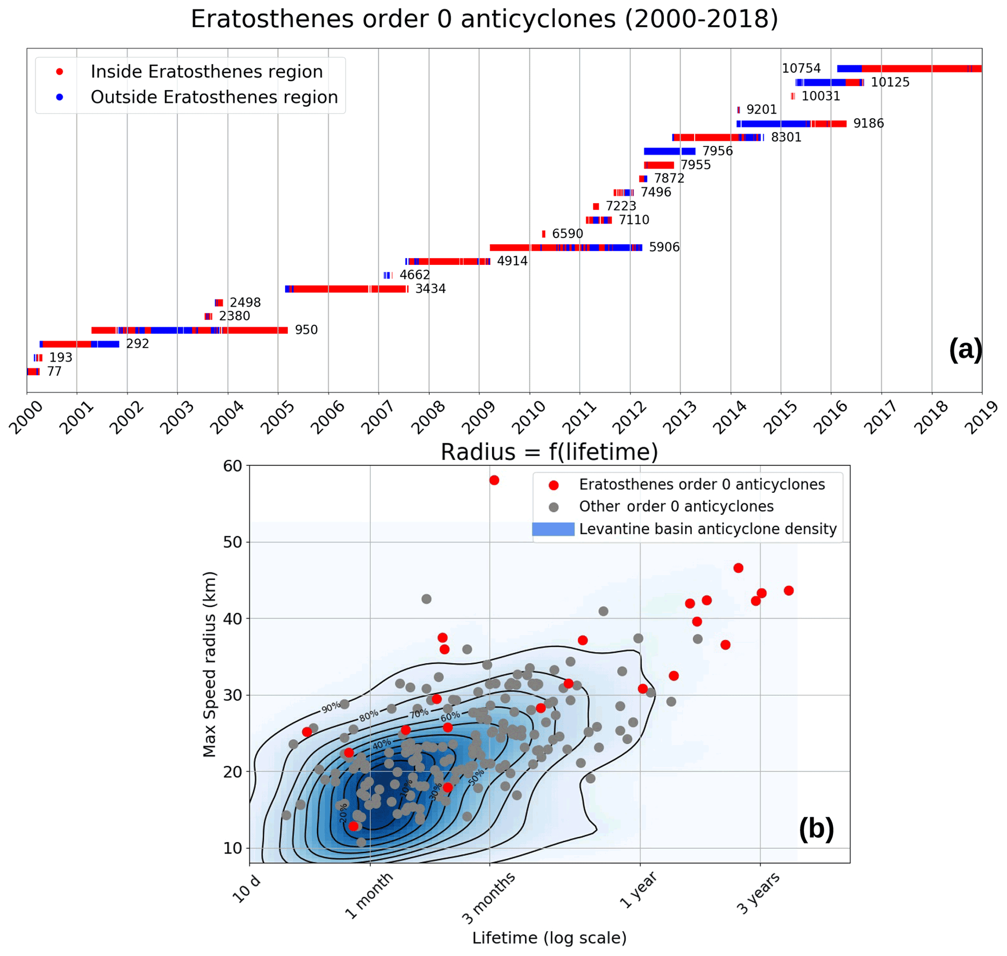
Figure 8 Details of the anticyclones constituting the EAA, detected as order 0 for the Eratosthenes region (tracks in Fig. 2a). (a) Time series with the eddy ID number from the DYNED database. The colored marker indicates when the eddy center is within (red) or outside of (blue) the region. (b) Scatterplot of the maximum speed radius as a function of lifetime, on a logarithmic scale, for order 0 anticyclones of the Eratosthenes region (red dots) and the other regions (gray dots); the blue shaded background is the density function for all LB anticyclones – except the Eratosthenes anticyclones – with contours each 10 % probability step.

4.4 Anticyclones detachments from the Levantine coast

In Sect. 4.3, the Eratosthenes attraction basin was identified, notably attracting anticyclones originally formed near the Levantine coast as seen in altimetric tracks (see Fig. 6a). However, altimetric eddy detections have important limitations stemming from the large spatiotemporal interpolation between satellite measurement tracks. This makes the resolution of altimetric maps ($\mathrm{1}/\mathrm{8}$^∘ in the Mediterranean Sea) insufficient to adequately detect small-scale structures and introduces uncertainty in the detection, especially as the internal deformation radius is small (Le Vu et al., 2018). Nevertheless, other sources of satellite images such as SST contain visible eddy signatures on them (Moschos et al., 2020). On such images, we can observe filament exchanges between eddies as well as eddies moving too fast to be detected via altimetry, such as the eddies detaching from the Levantine coast. Gertman et al. (2010) spotted such a detachment in August 2009 by means of in situ data from drifting buoys. Here, we provide observational evidence from SST images of a similar event occurring on July 2016: a detached warm-core anticyclonic ring, part of a cyclone–anticyclone dipole, rapidly merged with another anticyclonic eddy that later subsequently merged with the Eratosthenes anticyclone. Figure 9 portrays this event through four daily SST image snapshots where the altimetric detection DYNED contours have been superimposed. An anticyclone not detected by surface altimetry with a particularly warm surface signature can be spotted on the right-hand side of Fig. 9a (17 July 2016). A cyclone with which it forms a dipole can be seen from the SST in its southeast corner and is also detected by the altimetry somewhat more southwards. In Fig. 9b, 5 d later (22 July 2016), this anticyclone has moved rapidly towards the DYNED anticyclone no. 10754, which was first detected offshore of Haifa on 10 February 2016. The track of DYNED anticyclone no. 10754 is depicted using a blue line. The warm-core detached anticyclone will eventually merge with it 6 d later (28 July 2016; Fig. 9c). A month later (2 September 2016; Fig. 9d), this anticyclone will eventually merge with the eddy on the Eratosthenes Seamount, having transferred the warm waters and the momentum of the detached warm-core eddy.

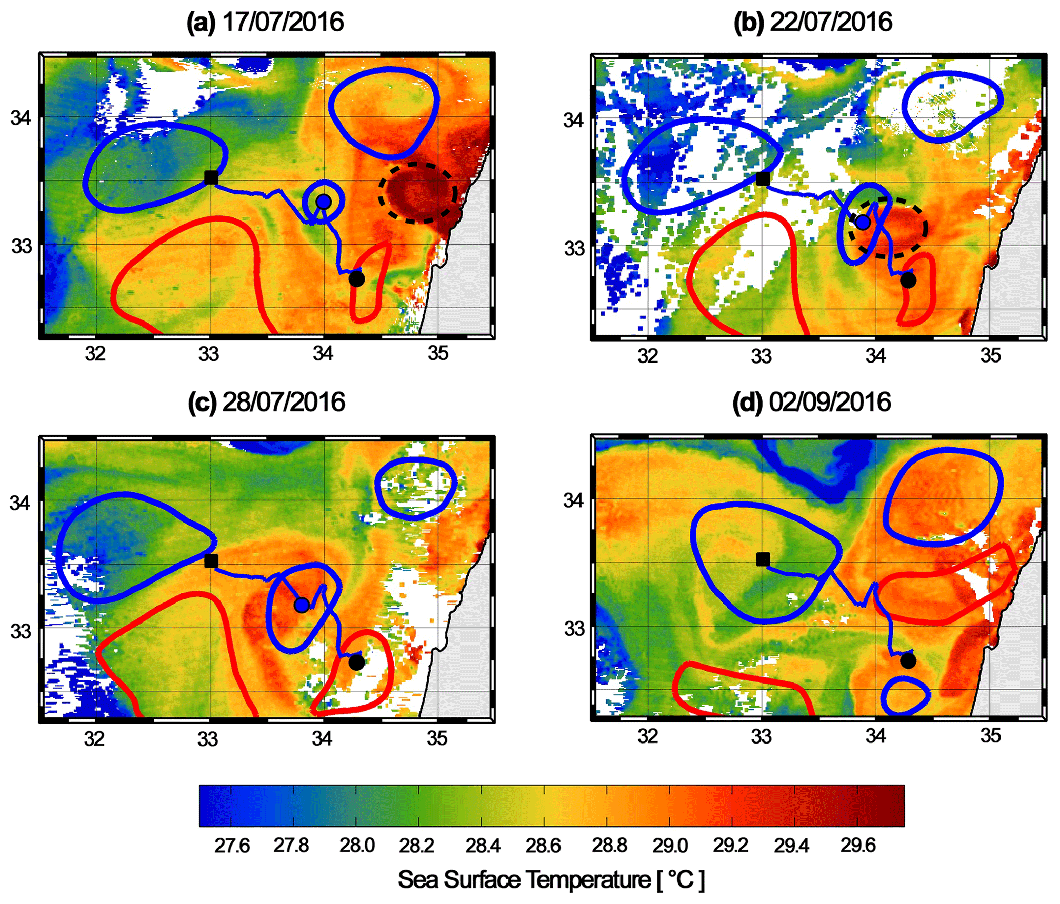
Figure 9 Daily snapshots of SST images showing a quickly moving warm-core anticyclone, part of a dipole that detaches from the Levantine coast and merges with a future Eratosthenes anticyclone. Superimposed DYNED contours are blue for anticyclones and red for cyclones. The track of the studied anticyclone is shown in blue line, its current center is shown using a blue circle, its initial detection on 10 February 2016 is shown using a black circle and its last detection on 2 September 2016 is shown using a black square. A blue line approximates the track of the warm-core anticyclone as seen in the SST sequence.

4.5 Marsa Matruh attractor

Eddy attraction to the other big anticyclonic structure of the region, called “Marsa Matruh”, can be studied in comparison to the Eratosthenes attractor. In Fig. 10, the Lagrangian framework defined in Sect. 3.1 is applied to this region. Firstly, it is notable that this structure clearly also acts as an attractor, with the total number of importing eddies (sum of orders 0–1–2) being a lot higher than order 0 alone and exporting eddies. In a similar fashion to the Eratosthenes region, which acts as a stranding place for anticyclones detached from the Levantine coast, a lot of the anticyclones that are detached from the Libyo-Egyptian coast (likely as instability of the Libyo-Egyptian current) end in the Marsa Matruh region, often through one merging event or more. In particular, a hotspot of anticyclone formation takes place in the Marsa Matruh gulf at approximately 31.5^∘ N, 27.5^∘ E, from which five anticyclones drifted towards the Marsa Matruh structure. No importing anticyclones come from the north, as expected given that almost no anticyclones occur in the Rhodes gyre (see Fig. 4a).

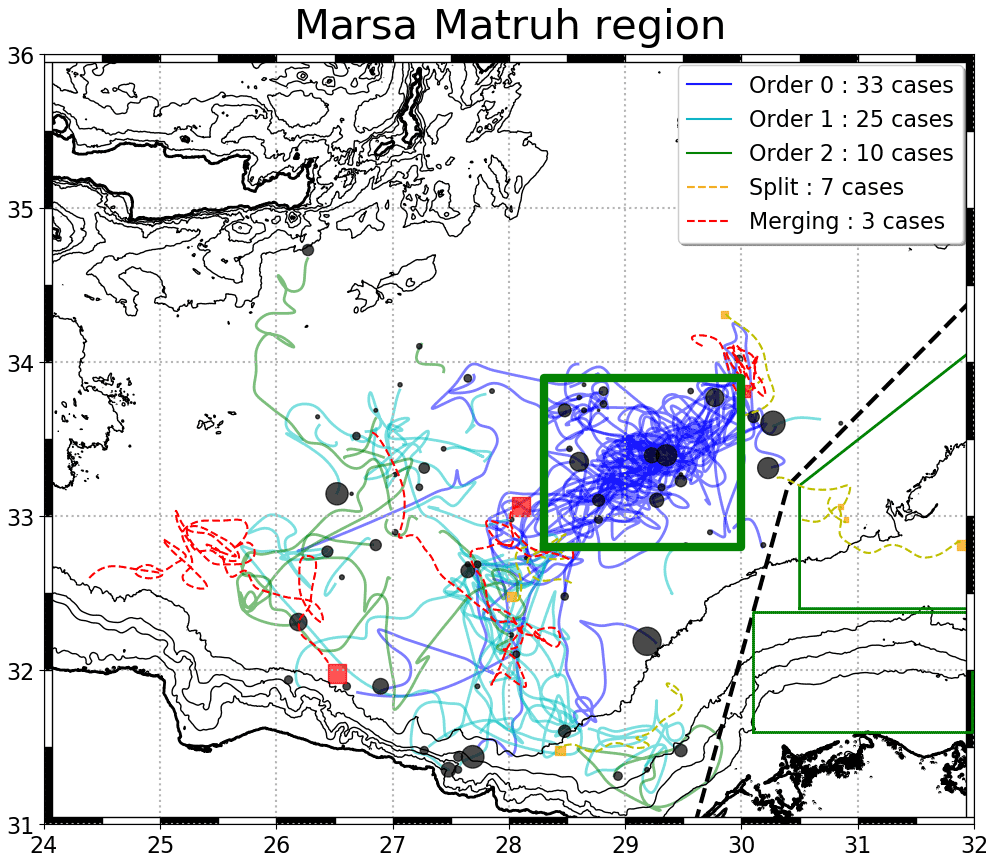
Figure 10 Convergence structure applied to the Marsa Matruh region, administered in the same way and using the same color code as in Fig. 6.

However, in contrast to the Eratosthenes attraction basin which is isolated with very few anticyclone exchanges outside, the Marsa Matruh anticyclone has no clear western boundaries. For instance, some merging export trajectories in red are present southwestwards, highlighting that some eddies escaped from this structure. On the contrary, one Ierapetra eddy did end through successive merging events into the Marsa Matruh area. This individual event seems to be isolated, as shown in Ioannou et al. (2017), Ierapetra eddies actually tend to go westwards, riding up the Libyo-Egyptian current, if they move away, in a similar way to the eddy behavior described by Sutyrin et al. (2009). More generally, the importance of higher-order anticyclones merging in successive steps to the Marsa Matruh anticyclone suggests that convergence is less straightforward and clear than for the EAA, likely because topographic constraints are less present.

5 Vertical structure of the Eratosthenes anticyclone attractor

The DYNED-Atlas co-localization and background method (see Sect. 3.3) is used to estimate the heat, salt and density anomalies associated with each eddy. For very persistent long-lived eddies, such as those constituting the EAA, this allows one to observe changes in the vertical structure and the evolution of the associated anomalies. Figure 11 shows the annual averaged vertical profiles of the Eratosthenes attractor, over all available profiles within each year and closer than 30 km to the eddy center, for different years during the 2000–2018 period. A histogram below indicates how many profiles are available for each year. This number varies a lot due to the inconstant frequency of oceanographic surveys, with the years from 2008 to 2011 being overrepresented because of extensive glider sections (Hayes et al., 2011) and several Argo floats being trapped for a very long time inside the anticyclone.

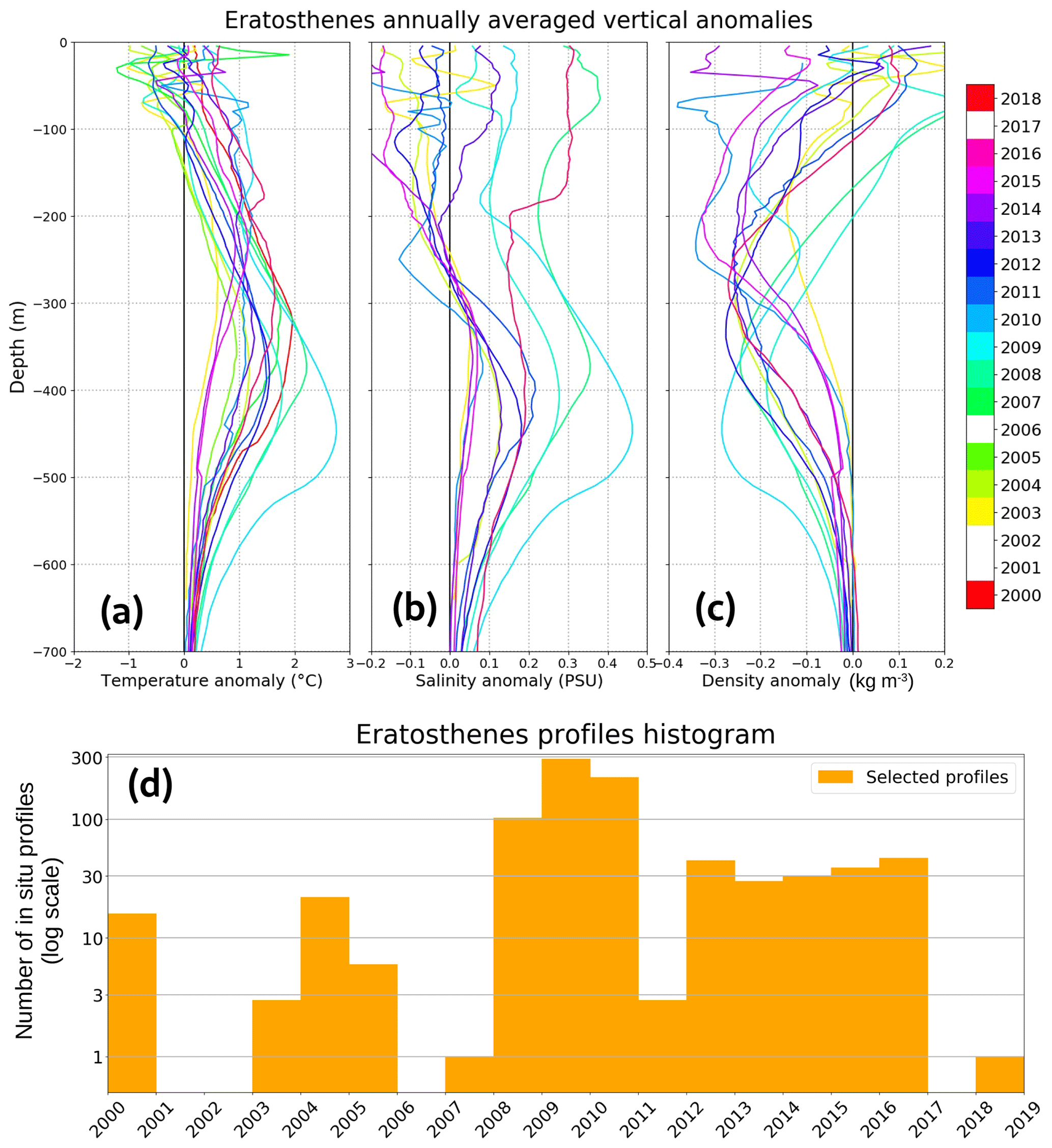
Figure 11 The annually averaged vertical profiles anomalies for (a) in situ temperature, (b) salinity and (c) density, inside Eratosthenes order 0 anticyclones. Profiles are selected if they are cast within 30 km of the eddy center, and their histogram is shown in panel (d) on a log scale. Years without any profiles are discarded from the color bar. Some years (e.g., 2005) only present a temperature profile, as only XBT casts were available.

In the annual averaged vertical profiles in Fig. 11, the EAA anticyclones can be characterized by very deep anomalies, both in salt and temperature. For every year, the depth of maximal density anomaly is below 200 m, and it reaches 450 m some years. The magnitude of the anomalies can also be extremely marked, higher than +2.5 ^∘C and +0.45 PSU in 2010. However, if annually averaged temperature anomalies always reach +1 ^∘C at 200 m or below, Fig. 11 shows that there is a strong interannual variability in the vertical structures of these anticyclones. The year 2010 then appears as an extreme event, with the formation of a double-core structure visible on the density profile (Fig. 12c). This event was surveyed by gliders and described by Hayes et al. (2011); however, with longer time series, it can be seen that eddy-induced anomalies in 2009–2010 were extreme compared with the 19-year mean vertical structure.

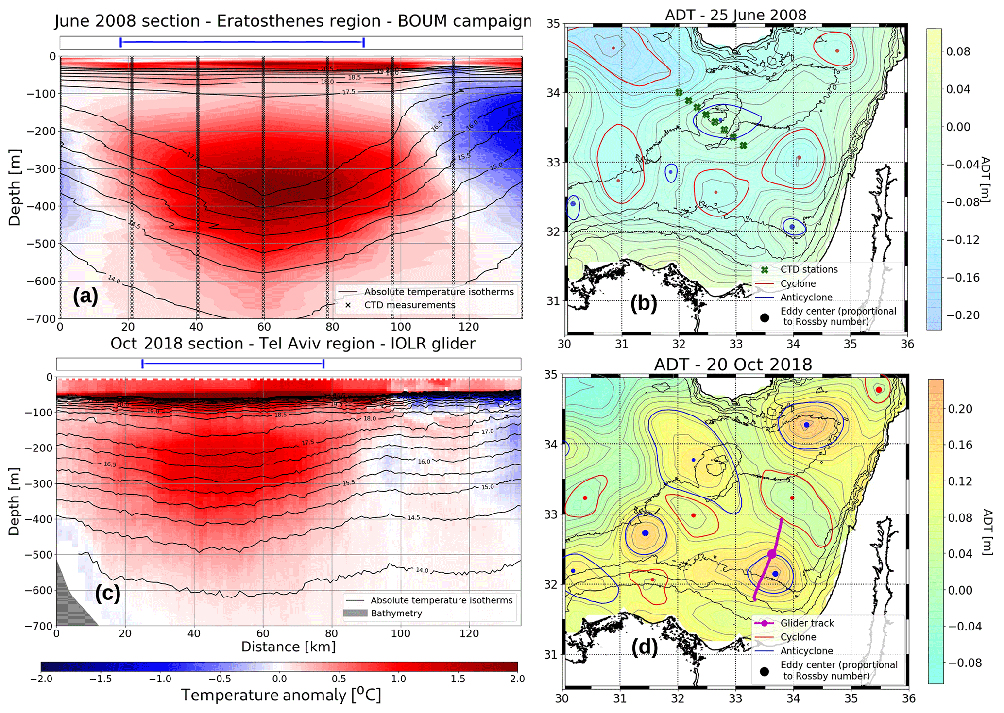
Figure 12 Comparison of anticyclone sections. The Eratosthenes (a) and Tel Aviv (c) region anticyclone sections in June 2008 and mid-October 2018, respectively. The left side is northwards, the horizontal axis (shared) is the distance along the section, black lines are the absolute temperature isotherms, the temperature anomaly is shown using the colored background and the blue cartridge above the panel outlines the limits of the eddy contours. Panels (b) and (d) show the respective ADT maps at the corresponding date of cast, presenting the neighboring eddy activity. Green crosses (a magenta line) show the CTD casts (the glider track). The eddy contours are maximal speed contours – blue denotes the anticyclones, red denotes cyclones and there is a Rossby number-scaled dot for their center.

In the BOUM campaign in 2008, Moutin and Prieur (2012) also compared the vertical structure of an Eratosthenes anticyclone with two other anticyclones in the Mediterranean Sea: a detached Algerian eddy and an anticyclone in the central Ionian Sea. Their comparison showed that the anticyclone constituting the EAA had the deepest potential density maximal anomaly (at 380 m compared with 160 m in the Algerian eddy) and that integrated anomalies were very warm and salty waters, with respective temperature and salinity anomalies of +2.35 ^∘C and +0.388 PSU (+0.75 ^∘C and −0.65 PSU in the Algerian eddy). Such values are consistent with observations in other years, as shown in Fig. 11b–c, although slightly higher.

The vertical structure of Eratosthenes anticyclones described above should be compared with physical properties of neighboring eddies in the LB. Figure 12 presents the comparison between a section representative of the Eratosthenes anticyclone, using data from the BOUM campaign in June 2008 (Moutin and Prieur, 2012), and an anticyclone section in the Tel Aviv region performed in October 2018 by a glider from IOLR. Next to each section is an ADT map representative of the SSH activity at that time (Fig 12b, d). The glider section lasts for 10 d, with 20 October 2018 being the median date; a magenta line indicates the glider track, and the position on the 20 October is shown with a magenta circle. The daily altimetric eddy contours are plotted on the ADT maps, with cyclones in red and anticyclones in blue, and a dot with a size proportional to the vortex Rossby number indicates the center. The upper panel of each section (Fig. 12a, c) marks the part of the cross section that is inside the maximal speed anticyclone contour using a blue line. Thin black lines in the vertical sections are the absolute temperature isotherms, whereas color indicates the temperature anomaly relative to the climatological background; the isotherm intervals and the color bar range are the same in both sections for comparison purposes. An important difference is that Fig. 12a is an interpolation between the CTD measurements (indicated by black crosses), whereas Fig. 12b shows a glider track stacking in which each pixel corresponds to a measurement.

Although a 10-year period separates the two sections, it should first be noted that the local eddy activity is similar in both events and is very close to the mean circulation deduced from Fig. 1: anticyclones are found in Eratosthenes, Herodotus and Tel Aviv regions, whereas a cyclone is found in the Haifa region. Furthermore, as can be seen in the ADT maps, both sections crossed the anticyclones close to their respective center, allowing one to assume that the maximal anomaly was adequately sampled. Extensive glider sections were surveyed in the Eratosthenes region in 2009 and 2010, but as explained above, 2010 appears as an extreme year where comparison with neighboring eddies will be biased.

The anticyclone constituting the EAA surveyed in Fig. 12a is a long-lived anticyclone, referenced in the DYNED database as no. 4914, born in the Beirut region before settling over the Eratosthenes Seamount for more than 6 months. The Tel Aviv eddy measured in Fig. 12c is a young anticyclone formed close to the shore in August 2018, as detected by AMEDA at approximately 32.0^∘ N, 34.0^∘ E and referenced as DYNED no. 12683. It drifted slowly offshore northwestwards before dying without merging at approximately 32.5^∘ N, 33.0^∘ E at the beginning of December 2018. It is, therefore, very similar to the anticyclones formed in the Tel Aviv region and drifting offshore, sometimes merging in the Eratosthenes region, in a similar way to the trajectories shown in Fig. 6c. In both events, the Tel Aviv anticyclone appears to be more intense in terms of Rossby number than the Eratosthenes anticyclone (as shown by a larger dot on the ADT maps), but the vertical structure shows that the Eratosthenes anticyclone, although weak in altimetric signature, hides a very deep and strong temperature anomaly: +2.35 ^∘C at 380 m compared with +1.3 ^∘C at the depth of the maximal density anomaly of 250 m in the Tel Aviv anticyclone. This comparison shows that anticyclones in the EAA can also be differentiated from neighboring eddies by a deeper subsurface anomaly, consistent with first observations by Stegner et al. (2019), who showed that the depth of the maximal density anomaly over the Eratosthenes Seamount (often below 300 m) is an almost unique specificity in the whole Mediterranean Sea.

6 Discussion

With only 3 years of SST data, Hamad et al. (2006) showed that along-shore current instabilities create eddies drifting offshore, and they identified the Eratosthenes Seamount as an anticyclone accumulation area (see their Fig. 16). In this study, with the hindsight of 19 years of eddy tracking, we add a quantification of the importing eddy flux and confirm what was previously inferred through a limited time period of data. We also observe that anticyclones are actually often formed offshore close to the seamount in the west, in the region referred to as “Herodotus” in this study.

Another important result of the eddy tracking performed here is the isolation of anticyclone dynamics from the rest of the LB: almost no anticyclones come from areas further west than the Herodotus region and, conversely, almost none escape this attraction basin (dashed black line on Figs. 3, 4, 6a–g and 7). It can be noted in Fig. 4a that the dashed line coincides with anticyclone drift divergence. This observation is not true for cyclones; however, as they do not have a thick core of homogeneous water and have significantly shorter lifetimes than anticyclones (see Fig. 5), they are assumed to contribute less to water mass transport. This western impermeable border could be linked to the presence of the Mid-Mediterranean Jet (MMJ). Zodiatis et al. (2010) suggested that this jet could be feeding the Eratosthenes anticyclonic structure. Nevertheless, the jet could also act as a barrier for anticyclones, explaining the absence of an anticyclone flux from the Marsa Matruh area into the Eratosthenes region (see Fig. 6a).

In older literature, Robinson et al. (1991) discussed the hypothesis of a northern path of Atlantic waters in the LB, isolating its southeastern part but grouping together the Marsa Matruh and Eratosthenes structures. This analysis was performed with a hydrographic vision using CTD stations. More recently, Ayata et al. (2018) carried out a review of the Mediterranean regionalization across eight studies using various parameters, mainly with a biological or hydrological focus. A remarkable result from this review is the very good agreement of these studies with respect to distinguishing a region of homogeneous properties in the southeastern LB, called “Levantine”. The region proposed by the authors (see Fig. 4 in Ayata et al., 2018) matches very well with the borders of the EAA attraction basin delineated in this study, apart from the edge along the Egyptian and Levantine coasts. Thus, these results suggest a real hydrographic significance of the EAA attraction basin and a possible role of anticyclones in homogenizing water masses properties.

Additionally, given the importance of this area for intermediate water formation, the fate of water masses in the EAA core and its dissipation would be of great interest for extended research. Anticyclones coming from different formation areas regularly merge with the EAA, and the imported water masses should, therefore, be transported. They likely feed its subsurface anomaly, which was shown to be deeper than surrounding structures (see Fig. 12), but the final destination of these waters is unknown. Erosion from its deep anomaly due to intense shear from topographic interaction with a seamount (Sutyrin et al., 2011) could provide a warm and salty water flux at depth, leading to the formation of intermediate water masses. Answering this very important question requires further simulation work as well as more in situ oceanographic data forming a consistent and continuous three-dimensional time series to accurately follow its evolution.

This study reveals the existence of the EAA from the analysis of eddy tracks, but questions remain regarding the mechanisms explaining this anticyclone convergence, whereas more classical westwards β-drift (Chelton et al., 2011) or current advection along the coast (Sutyrin et al., 2009) could be expected. There is controversy regarding whether the EAA effectively attracts other eddies or, conversely, if eddies detach from the coast and merge with a central and long-lived structure. In other words, does the EAA pull other anticyclones towards the seamount (in an active way) or is it acting as the stranding point of anticyclones advected by the mean flow (in a passive way)? SST images and detachments observed from the coast, shown in Fig. 9 in this study but previously observed in the literature by Hamad et al. (2006) and Gertman et al. (2010), suggest that the second option is likely happening. On the other hand, the high occurrence of eddy merging and splitting highlights the importance of eddy–eddy interactions in this basin. Further studies in this direction are needed to outline eddy dynamics, although the small internal deformation radius in the Mediterranean Sea of 10–12 km (Mkhinini et al., 2014) only allows one to accurately detect large mesoscale structures. Nevertheless, great improvements are possible via the application of eddy automatic detection at smaller scales than the mesoscale with the help of SST data (Moschos et al., 2020).

The presence of the EAA over a seamount obviously raises the question of topographic interactions. Two attractor structures are observed in the LB, over very different bathymetry: the Marsa Matruh attractor over the Herodotus Trench deeper than 2000 m and the EAA over the Eratosthenes Seamount whose summit is approximately 700 m deep. This similarity suggests that interactions with the seamount do not play a significant role in anticyclone convergence towards the EAA, and if significant, the presence of a seamount should actually destabilize anticyclone dynamics (Sutyrin et al., 2011). However, some differences between these structures (see Sect. 4.5), notably the more variable average position or attraction basin of Marsa Matruh, could be explained by topographic interactions.

Last but not least, the background used to estimate eddy vertical structure in Sect. 5 is considered a climatological reference at the same approximate location and time of the year (see Sect. 3.3). However, it is computed as a 2000–2018 average and could then be altered by events of strong interannual variability, reported in the LB by Ozer et al. (2017). Long-term evolution of the eddy-induced physical property signature deserves further work.

7 Conclusions

Using the DYNED-Atlas database of eddies in the Mediterranean Sea, a Lagrangian convergence method is defined, and its application to anticyclone tracking from 2000 to 2018 enables one to quantify anticyclone transfers between subregions of the southeastern LB. At the position of a known area of anticyclone accumulation, it reveals the existence of anticyclone convergence toward the Eratosthenes Seamount in a structure that we named the Eratosthenes anticyclone attractor. This attractor proves not to be a single fixed anticyclone but is rather constituted by a succession of long-lived anticyclones sharing dynamical characteristics, distinct from neighboring eddies: longer lifetime – more than 1 year and up to 4 years – and a maximal speed radius above 40 km – more than 3 times the internal deformation radius. Lagrangian eddy tracking also showed that the convergence towards the EAA is geographically bound to a clear attraction basin. Anticyclones drift towards the Eratosthenes Seamount after detaching from the current along the Levantine coast or being formed westward in the region that we named Herodotus. The formation of anticyclones with a short lifetime quickly merging with the EAA are spotted in the regions called Tel Aviv and Haifa. An effective barrier for anticyclones is then found between the Eratosthenes and Marsa Matruh regions. In situ vertical profiles are co-localized with eddies, and climatological backgrounds are computed using the DYNED-Atlas method, allowing one to estimate the eddy-induced physical property signatures. The anomalies induced by the anticyclones constituting the EAA are found to be extremely deep, with depths of maximal density anomaly always at or below 200 m, reaching 450 m in some years, but with pronounced interannual variability. Annual averages of the temperature anomaly are found to be always equal to or greater than +1 ^∘C at 300 m, revealing a large heat storage capacity of the anticyclone.

Appendix A

Figure A1 Sensitivity of the total number of order 0 anticyclones with the lifetime criterion, for four chosen regions: “100 %” means that order 0 anticyclones are strictly the ones dying in the study region; “30 %” means that order 0 are dying in the study region as well as anticyclones that spend 30 % of their lifetime within the borders of this region. A value of 50 % is chosen in this study (see Table A2).

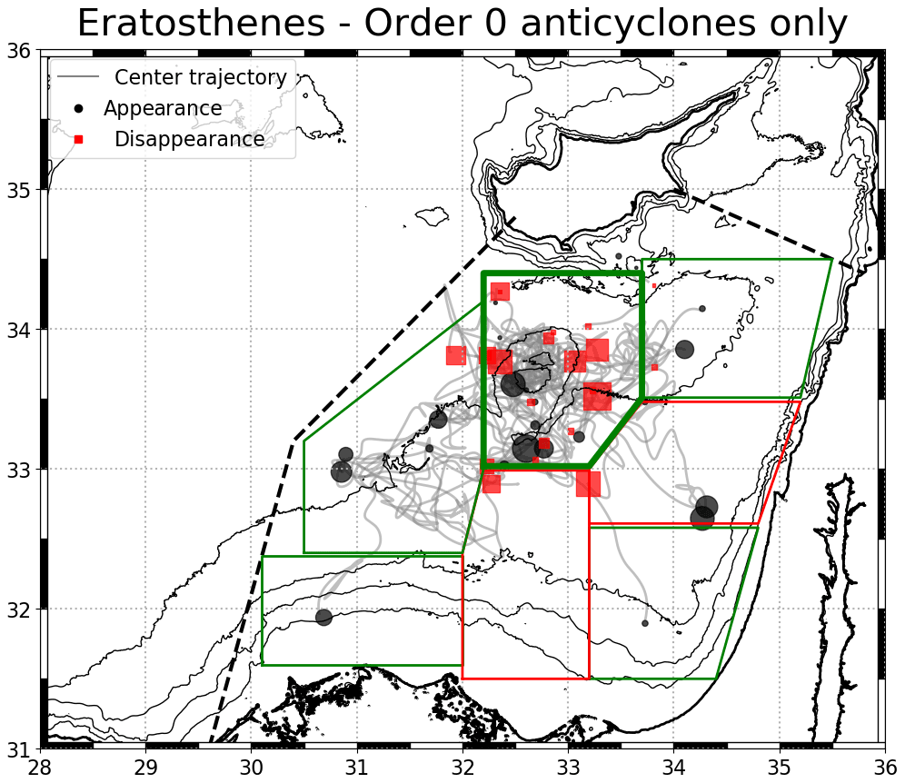
Figure A2 Appearance and disappearance locations for all order 0 anticyclones for the Eratosthenes region. Even if not all of them die within the region, they disappear very close to it.

Figure A3 Cyclone transfers for Haifa region. Same as Fig. 6c but with the Lagrangian convergence framework applied to cyclones. Boxes and dashed line are the same as in Fig. 3.

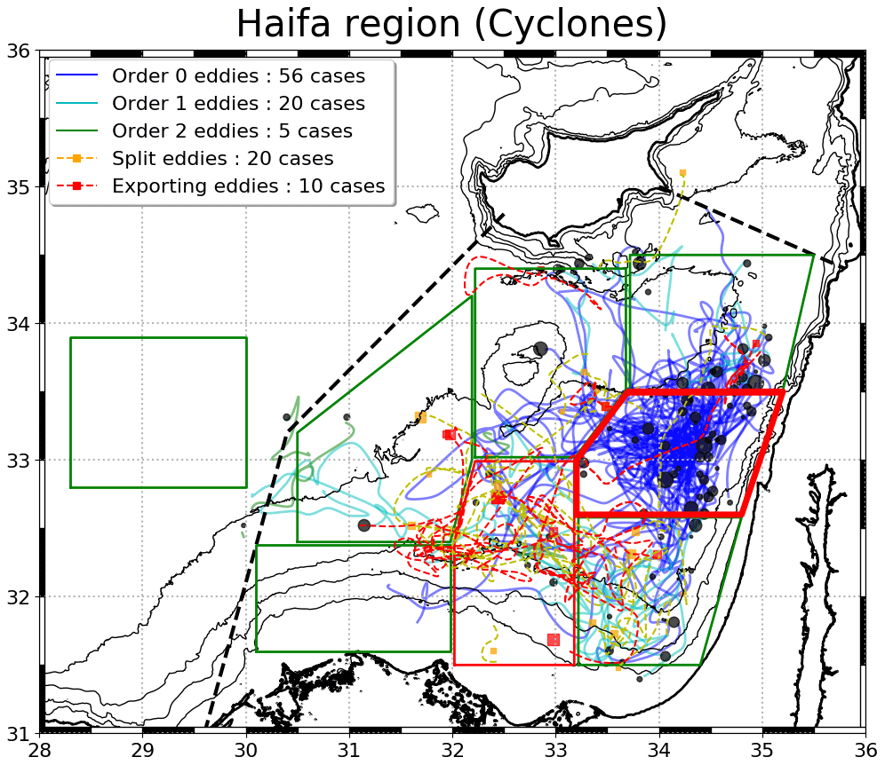
Table A1 Regions studied in the LB, showing the coordinates and area. Corresponding boxes are shown in Fig. 3.

Table A2 Details of importing and exporting anticyclones for the seven regions of the southeastern LB identified in Sect. 3.2. Details are also shown in Fig. 6a–g, and the net anticyclone gain appears in Fig. 7.