Temporal and spatial variations in three-dimensional seismic oceanography

Seismic oceanography is a new cross-discipline between geophysics and oceanography that uses seismic reflection data to image and study the oceanic water column. Previous work on seismic oceanography was largely limited to two-dimensional (2D) seismic data and methods. Here we explore and quantify temporal and spatial variations in three-dimensional (3D) seismic oceanography to address whether 3D seismic imaging is meaningful in all directions and how one can take advantage of the variations. From a 3D multichannel seismic survey acquired for oil and gas exploration in the Gulf of Mexico over a 6-month period, a 3D oceanic seismic volume was derived. The 3D seismic images exhibit both temporal and spatial variations of the ocean, and theoretical and data analyses were used to quantify their contribution. Our results suggest that temporal variation is more prominent in the crossline direction than in the inline direction, causing discontinuities in crossline images. However, a series of 3D inline images can be seen as snapshots of the water column at different times, capturing temporal variation of thermohaline structures induced by ocean dynamics. Our findings suggest the potential uses of marine 3D seismic data in studying time-evolving mesoscale ocean dynamics.

1 Introduction

Despite being the Earth's largest habitat by volume, the ocean water column remains one of the most poorly explored environments. Even where investigations are executed, physical, biological, and chemical parameters are generally derived from one-dimensional (1D) profiles (e.g., CTD casts, buoys, and moorings) or two-dimensional (2D) transects (e.g., underwater gliders). Capturing the three-dimensional (3D) structure of the water column is extremely complicated: it can be reconstructed for a very large volume by combining 1D and 2D measurements or, in a capacity limited to surface waters only, it can be inferred from satellite observations. Also, mesoscale and small-scale thermohaline fine structures are very difficult to observe with conventional methods whose lateral resolutions are coarse (usually > 100 m). The ocean interior is 3D by nature and varies in both time and space on a wide range of scales. Ocean dynamics such as internal waves, solitons, tidal beams, eddies, and fronts (that affect thermohaline fine structures) are expected to vary both spatially and temporally. Currently, seismic oceanography using marine seismic reflection data to image ocean structures is the only method by which we can collect high-resolution 3D information about the oceanic wave field. In this work, we aim to understand how temporal and spatial oceanic variability is distributed in 3D seismic images, a critical question in making the best use of 3D seismic oceanography.

Previous studies showed that seismic reflection data, which were commonly used by geophysicists and geologists to image the Earth beneath the seafloor, can also produce surprisingly detailed images of water-column structures. Holbrook et al. (2003) and Holbrook and Fer (2005) demonstrated that 2D seismic reflection sections, if appropriately processed, provided high-resolution images of the ocean structure, both vertically and, in particular, horizontally. Within the ocean water column, density variations, fine-scale (1–10 m thickness) temperature–salinity contrasts, and turbidity fluctuations result in small changes in sound speed that produce distinct sound reflections. These reflections, 100 to 1000 times weaker than those from the solid earth below, have generally been neglected by geophysicists, whose focus is the structure of the sub-seafloor. However, studies reveal that these reflections correspond to ocean thermohaline structures (Nandi et al., 2004; Nakamura et al., 2006) and are primarily (not completely) associated with temperature gradient (Ruddick et al., 2009). This new cross-discipline, between exploration seismology and physical oceanography, has come to be known as seismic oceanography (Holbrook et al., 2003) and has been successfully applied to imaging mesoscale and sub-mesoscale water-column structures such as ocean fronts (Gorman et al., 2018), eddies (Song et al., 2009; Tang et al., 2014a), internal waves (Holbrook et al., 2009; Tang et al., 2014b; Buffett et al., 2017), and other thermohaline fine structures (Holbrook et al., 2003). Additionally, several theoretical studies have been derived from the application of water-column seismic images including estimation of geostrophic currents (Sheen et al., 2011; Tang et al., 2014b), wave field spectra (Fortin et al., 2016), and internal wave mixing (Dickinson et al., 2017). Most of these studies used 2D seismic data and processing methods, but in the modern exploration seismology of the oil and gas industry, 2D seismic methods are gradually upgraded to 3D seismic methods, which provide improved seismic images with the help of the additional dimension, leading to a more reliable interpretation (Yilmaz, 2001).

3D seismic surveys are distinguished from 2D seismic surveys by the contemporary acquisition of multiple closely spaced lines (e.g., 25 m) that provide regular data point spacing. This survey configuration leads to a true data volume from which lines, planes, slices, or probes can be extracted in any orientation, with nominally consistent data processing characteristics. While it is possible to acquire a dense, high-resolution grid of 2D lines, such grids are fundamentally different from a native 3D seismic survey (Lonergan and White, 1999; Yilmaz, 2001). The close spacing of 3D seismic lines and the physical illumination of the subsurface from multiple parallel receiver arrays remove spatial aliasing problems inherent to 2D seismic data. Therefore, 3D seismic oceanography has the potential to yield higher spatial resolution and can be useful for studying the orientation of ocean structures (Blacic and Holbrook, 2010). To date, 3D seismic oceanography is still not well developed, which might be due to multiple factors: the 3D seismic data are very expensive to acquire, there is an interdisciplinary gap between oceanography and geophysics, and, most importantly, a fundamental understanding of the capability of 3D seismic oceanography is missing.

The fundamental principle of exploration seismology assumes only spatial and not temporal variations in the sub-seafloor (at least in the survey time frame). However, this challenges the development of 3D seismic oceanography, as 3D seismic surveys are generally acquired over a long period (e.g., from hours to months) and the water column may evolve during the collection of 3D seismic data. Recently, 3D seismic oceanography moved a big step forward, being successfully applied to explore the evolution of an oceanic front (Gunn et al., 2020) and the passage of an eddy (Dickinson et al., 2020). There are many fundamental questions regarding 3D seismic oceanography waiting to be answered. For example, how are temporal and spatial water-column variations distributed in a single 3D seismic volume? Can we quantify them? Is the oceanic 3D seismic imaging meaningful in all directions? The answers to these questions will be useful to guide the development of future 3D seismic oceanography.

In this study, we explore temporal and spatial variations embedded (i.e., variability that is predisposed to be recorded) in 3D ocean seismic volume and answer the fundamental questions mentioned above. We report results of a 3D seismic oceanography study carried out at the continental slope region of the northern Gulf of Mexico, where seismic imaging of ocean structures can be useful for understanding ocean dynamics and mixing. We analyzed multi-directional (inline, crossline, and depth-slice) seismic images to reveal fundamental imaging features. We further conducted theoretical and data analyses to understand the distribution of temporal and spatial variations. Our principal aim is to explore how 3D seismic data record spatial and temporal variability of the ocean. In this contribution, we focus on the potential of 3D imaging, rather than interpreting these oceanic phenomena. We aim to promote the development of 3D seismic oceanography, which is the only tool that can provide full-depth, high-resolution, 3D data of the ocean, by developing our understanding of how these data can be used to interpret the spatiotemporal evolution of ocean interior structure.

2 Data and methods

2.1 3D seismic data

Seismic data used in this study are a portion of a large multichannel 3D seismic survey conducted by Schlumberger WesternGeco in the northern Gulf of Mexico for oil and gas exploration between 2002 and 2003. Our study region (Fig. 1) is at the continental slope of the northern Gulf of Mexico, outside the Mississippi River delta, where the water dynamics are mainly dominated by the Loop Current and the Mississippi River outflows (Coleman, 1988; Sturges and Lugo-Fernandez, 2005). Although our seismic region is north of the Loop Current, it is still a high eddy-kinetic energy region due to the presence eddies and jets over the continental slope (Hamilton and Lee, 2005). Therefore, we expect this site to experience a range of temporal and spatial oceanic variability.

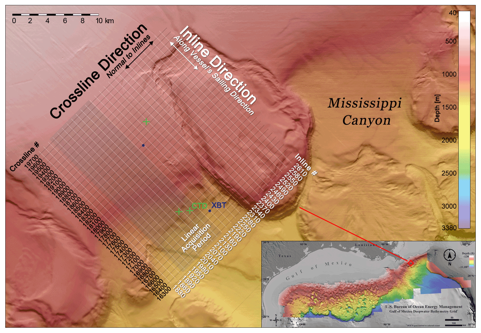
Figure 1 3D seismic survey area with inline (white) and crossline (black) configuration, CTD (green cross) and XBT (blue dots) locations, and seafloor topography (background color). The 3D seismic survey area is marked by the grids. Inline is oriented to go down the continental slope. The inset shows the survey location in the northern Gulf of Mexico. The seafloor topography data are provided by Bureau of Ocean Energy Management. The gray grids mark the linear acquisition period (explained in Sect. 2.4).

Seismic surveying lines run from northwest to southeast (inline azimuth, 330^∘) over a gentle continental slope (average inclination, 1.5^∘) where the seabed depth ranges from 800 to 1300 m. Seismic data were collected using two airguns of 5085 cubic inches, each in flip-flop configuration, and eight streamers, each accommodating 640 hydrophones. The streamer spacing was 100 m and the hydrophone spacing was 12.5 m. We received the raw shot gathers sampled at 2 ms and truncated at the seafloor with no processing applied apart from analog to digital anti-aliasing filtering (frequency range, 3–200 Hz). We received multiple CTD and XBT casts, including three CTD and two XBT casts inside the seismic area (see Fig. 1).

2.2 3D seismic data processing

Imaging the ocean water column using 3D seismic data from the oil industry is challenging. Acquisition geometry is not optimized for this target and ocean internal reflections are inherently weak and masked by noise of a different nature. However, oil industry contractors employ cutting-edge technology and therefore the obtained seismic data are generally of high quality. The seismic data processing began with reading the raw data that include the recorded outputs of all measuring instruments. The output is a time series that contains reflected signals and noise. The next step is to remove channels that show bad or null trace. To reduce the effect of long-range noise and keep computational costs low, we use the portion of the dataset that has the greatest signal-to-noise ratio (SNR), i.e., data within 4 km of the acoustic source. The strong seafloor signals were also excluded from processing to achieve a relative balance of amplitude levels. The data preprocessing used here employed standard techniques for sub-seafloor seismic imaging, as described in Yilmaz (2001) and adapted to work with the water-column specific issues. Typical marine noise was present in the water-column data, e.g., acquisition-related noise and unwanted non-reflected waves or reflection energy returns from previous field records. Environmental noises include wind, shipping activity, and inherent ocean noise. We designed a filtering strategy specifically tailored to remove or minimize as much noise as possible while preserving the weak signals of interest. Consequently, we used low-cut 5 Hz and high-cut 150 Hz Butterworth filtering after each processing step to attenuate noise. The unwanted direct waves interfered with the subtle internal reflections of the water column and complicated the imaging. We applied frequency–wavenumber (FK) filtering and radon filtering to fruitfully attenuate unwanted linear noise, previous shot effects, and seafloor contributions.

We processed the 3D data in a 3D fashion, which uses both inline and crossline data, rather than sequential 2D processing. The attenuation of seismic waves due to the spherical divergence was compensated using the conventional exponential gain function (with a power of 2). For velocity model building and offset effect removal, i.e., the normal move-out (NMO) correction, the data sort was converted to the common midpoints (CMP) between sources and receivers. Velocity model building was performed using a curve-fitting process to the reflections in each midpoint gather within a window of 1410 to 1590 m/s. An objective measure of coherence is needed to determine the best-fitting curve. Among the existing measures, we used the semblance norm (Neidell and Taner, 1971), which is widely used in seismic data processing. This process, which is technically called semblance analysis, provides the time domain root mean square (RMS) velocity model that is a processing parameter required for further steps of seismic imaging. Semblance maxima (i.e., coherence) were picked manually in a distance interval of every 250 m in both the inline and crossline directions. Other useful information such as sound velocities derived from CTD measurements was also used to calibrate the seismic velocity model when there is a mismatch between model and measurement. The CTD casts are high-resolution data that are used as guidance for picking the semblance maxima during velocity analysis. Consequently, the stacking and migration processes were performed as imaging steps using the RMS velocities. For stacking, all traces within a midpoint gather are summed to produce a zero-offset single trace with higher SNR. Sorting the stacked traces along inline or crossline sections provides the first interpretable seismic images. The last correction was to correct the effect of the dipping reflectors via seismic migration (Yilmaz, 2001) that automatically moves reflectors to their true position in the subsurface and improves the continuity of the images.

We have also tested and performed a powerful multi-parameter imaging technique known as the common-reflection-surface (CRS) method for stacking and enhancing the data and also to avoid signal stretch after normal move-out correction (Yilmaz, 2001). The size of the CRS stacking surface was, however, chosen conservatively small, particularly in the crossline direction (50 m), to avoid stacking traces from different swaths. The CRS showed improved results compared to the conventional CMP-based imaging especially along the inline direction (Bakhtiari Rad and Macelloni, 2020). Afterward, post-stack time migration was performed using the estimated RMS velocities to correct the dipping events. Finally, the data were time-to-depth converted using the estimated velocity function integrated with in situ sound velocity casts.

2.3 3D seismic volume

The obtained 3D seismic volume of the ocean interior is illustrated in Fig. 2, showing the “slicing” configuration of 3D inline, crossline, and depth-line seismic images. A 3D seismic volume is generally a 3D matrix in which seismic reflections are color-coded according to the reflection amplitude and polarity. Each seismic reflection in the seismic images represents an “interface” between two water layers with different acoustic impedances, stemming from different temperatures and salinities in the water column (Ruddick et al., 2009). Because a seismic survey can be acquired in any planar direction, the notation in geographic coordinates (i.e., latitude and longitude) is not adopted. Instead, the planar position is organized in inline (the northwest–southeast direction, which is down the continental slope) and crossline (perpendicular to inline; the northeast–southwest direction, which is along the continental slope on a broad scale); see Figs. 1 and 2. The volume has a spatial resolution of 6.25 m in the inline direction, 25 m in the crossline direction, and 6–7 m in the vertical direction (assuming a sound speed of 1500 m/s and considering the dominant frequency of the airgun signal in the water column is between 50 and 60 Hz). Our seismic volume shows only the portion of the water column below 200 m because the geometry of sources and receivers, optimized for deep subsurface targets (several kilometers below the seafloor), poorly image the shallowest portion of the water column (Piété et al., 2013). The signal-to-noise ratio (SNR) of our inline seismic images ranges from 8–10, using the formula of Holbrook et al. (2013).

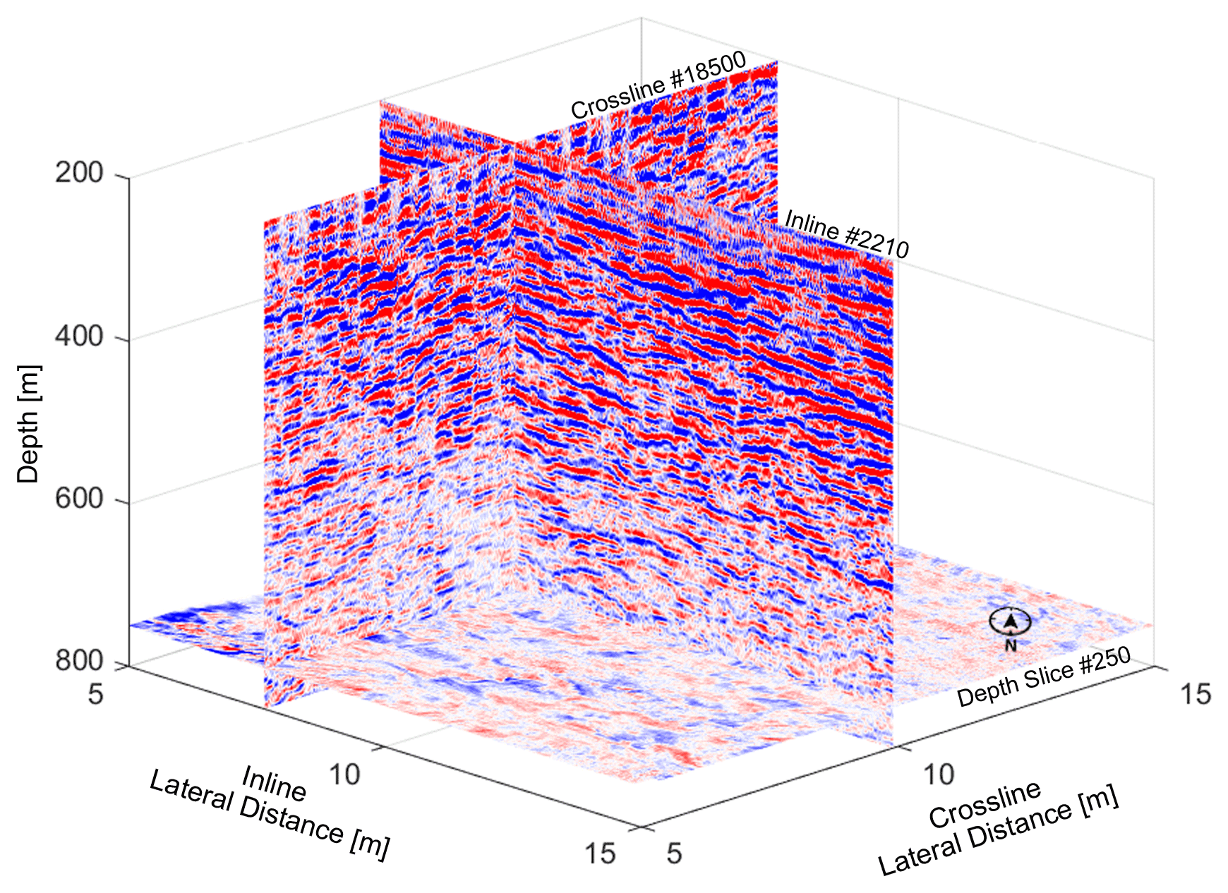
Figure 2 The inline, crossline, and depth-slice configuration in our obtained water-column 3D seismic volume in the Gulf of Mexico. The color represents the amplitude of seismic reflection.

For a 3D seismic oceanography study, inline sections are often acquired during short temporal intervals (typically a few hours considering the normal vessel velocity of 2.5 m/s). However, crossline sections, which are obtained by interpolating the inline sections perpendicularly, may embrace a wide temporal interval (from a few hours up to several months; the average interval is about 8 h within the linear acquisition period). We assume that water-column reflectors do not move during the shot and signal recording, i.e., the stick–slip model assumption (Klaeschen et al., 2009). Considering our inline collection time (a few hours) is smaller than the timescale of the mesoscale ocean dynamics (days), we assume that each inline represents a seismic snapshot of the water column. The entire 3D seismic volume extends for 480 km³ of the water column in the Gulf of Mexico. It consists of 821 inline sections, 3463 crossline sections, and 256 depth slices (5 m intervals vertically). Temporally, it covers over 6 months, from August 2002 to February 2003, with most collected between September and October.

2.4 Imaging capability analysis

To test if the 3D volume accurately images vertical temperature gradients of water-column structures, we compared the seismic reflections with the acoustic reflection coefficient derived by inverting the temperature–salinity curves collected along with the CTD profiles (Nakamura et al., 2006). The acoustic reflection coefficient for normal incident sound waves is given by (Kinsler et al., 1999)

$$\begin{array}{}\text{(1)}& R_s={\displaystyle \frac{{\mathit{\rho }}_{\mathrm{1}}{c}_{\mathrm{1}}-{\mathit{\rho }}_{\mathrm{0}}{c}_{\mathrm{0}}}{{\mathit{\rho }}_{\mathrm{1}}{c}_{\mathrm{1}}+{\mathit{\rho }}_{\mathrm{0}}{c}_{\mathrm{0}}}},\end{array}$$

where ρ₀, ρ₁ and c₀, c₁ are density and sound speed; the subscripts 0 and 1 specify adjacent layers. It has been widely demonstrated that the amplitude of seismic reflections is largely related to temperature gradients in the water column (Nandi et al., 2004; Nakamura et al., 2006; Ruddick et al., 2009), but sometimes salinity may play a role up to 40 % in regions prone to diffusive convection (Sallarès et al., 2009). Figure 3a compares the reflection coefficient derived from concurrent CTD measurements (collected on 17 October 2002, location shown in Fig. 1) with our seismic imaging (Inline #2130; seismic data collected on 17 October 2002). The overall agreement between the derived reflection coefficients with the seismic reflections suggests that our 3D seismic data successfully represents water-column thermohaline structures. Also, the derived reflection coefficient correlates highly (R=0.9970) with the temperature gradient (Fig. 3b), suggesting that the seismic amplitude in our seismic images can be interpreted as the vertical temperature gradient of the water column. In addition, the depth of the 3D volume seafloor reflection matches (within 5–10 m error) the seafloor depth from multibeam bathymetry, which is derived using highly accurate sound speed measurements collected by the NOAA ship Okeanos Explorer, confirming that our migration is correct and our seismic images accurately represent the water-column structure.

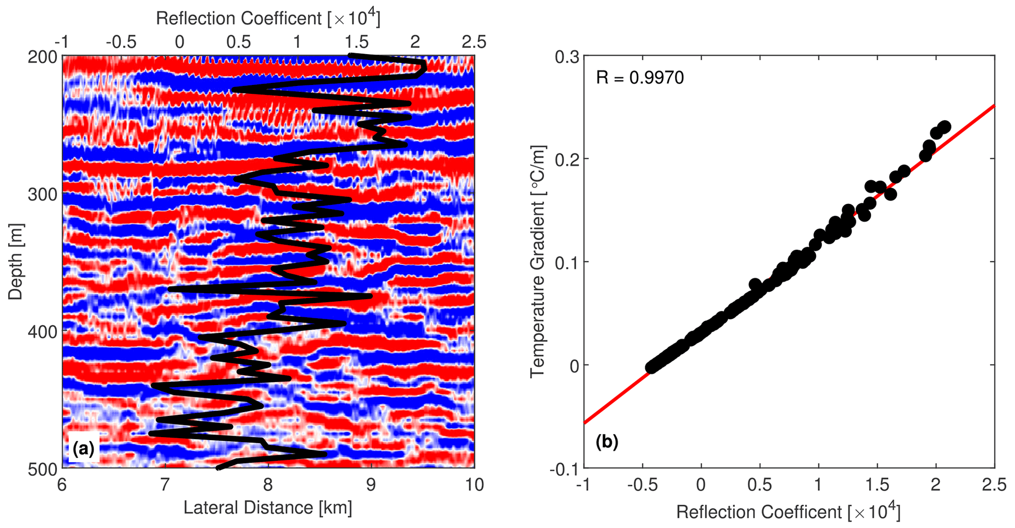
Figure 3 (a) Comparison of seismic imaging (Inline 2130) and the derived reflection coefficient (curve) from CTD data, both acquired on 17 October 2002. (b) Correlation between temperature gradient and the derived reflection coefficient between 200–1000 m.

2.5 Survey line distribution in space and time

Now that we have established the oceanic nature of these seismic reflections, we can describe the distribution of the seismic volume in space and time. We emphasize that inline sections are generally acquired during a short temporal interval (typically a few hours considering the normal vessel velocity of 2.5 m/s), while crossline sections, which are obtained by interpolating the inline sections perpendicularly, embrace a wide temporal interval, in our case up to several months. It has been demonstrated that water-column reflectors do not move during the very short time between the shot and the recording of the reflected signal (Klaeschen et al., 2009). In 3D surveys each shot is recorded simultaneously along with parallel streamers, generally referred to as swaths, which for our dataset count eight streamers. To better understand the temporal distribution of the inline or swath, we carefully investigate the acquisition time for each survey line by referring to the field acquisition records.

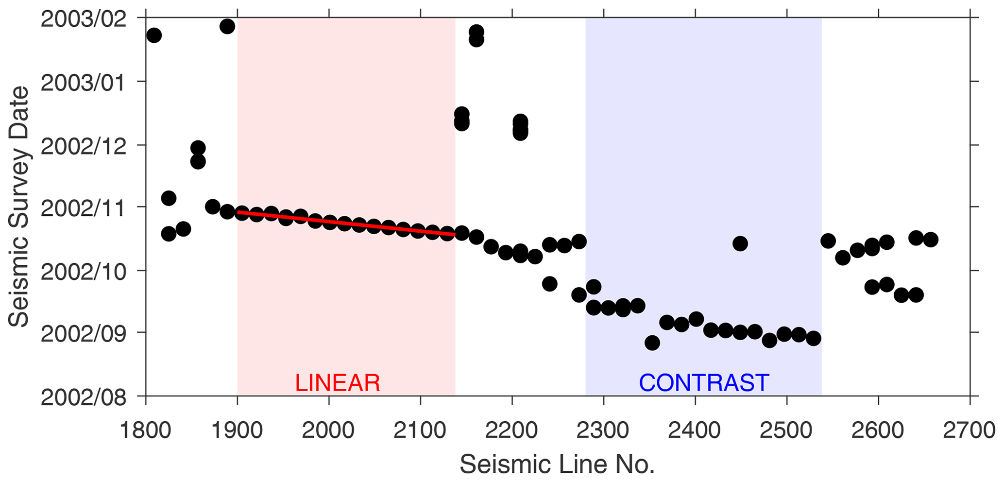
Figure 4 Dates of the seismic survey for the survey lines analyzed in our work. Two highlighted periods are a linear acquisition period (lines #1900–2140) during which data were collected linearly in time and space intervals, and a contrast acquisition period (lines #2280–2540), which can display a huge time jump in seismic image. The line number here is equivalent to the inline number at the center of a seismic swath.

Figure 4 shows the seismic line number, which is equivalent to the center inline number of a seismic swath, as a function of the recording date and time. Considering that 3D surveys are ideally carried out by acquiring adjacent swaths consecutively, we should observe a linear relationship between sailing line number and survey time. However, it is common that owing to operational problems (e.g., weather, maritime traffic, etc.) and/or bad data acquisition, some portion of the area may be covered at a different time or some lines may be reacquired. Figure 4 shows a general linear trend, in particular for the portion including lines 1900–2140. In this interval, spatially contiguous seismic lines were collected consecutively in time, yielding a crossline surveying speed of 1.5 swaths per day (equivalent to 0.6 km crossline imaging per day). We refer to this portion as linear acquisition period and we will use it in the correlation analysis discussed below.

3 Results

3.1 3D oceanic seismic images

In this section, we present multi-directional images from our 3D seismic volume to improve the understanding of water-column 3D seismic images and the fundamentals of 3D seismic oceanography and, hopefully, shed light on ocean dynamics that can be resolved from our seismic images.

Figure 5 shows three inline seismic images, each representing a snapshot along an inline transect in the linear acquisition period. We observe layers of strong seismic reflection in Fig. 5a, moderate reflection in Fig. 5b, and weak reflection in Fig. 5c, respectively, indicating vertical temperature gradients of the water column (see Sect. 2.4). Considering the spatial (2.5 km) and temporal (about 4 d) separations in these images, we observe that the water-column structures varied not only spatially (over 5 km) but, more importantly, temporally (over 8 d), suggesting a strong water-column mixing process may have occurred in this region. In other words, during the interval between 20–28 October 2002, over this portion (about 4 km) of the continental slope, the strong and thick thermoclines gradually weakened and thinned and eventually almost disappeared. We interpret the water-column variation as complex and diverse internal wave variation over the continental slope of the northern Gulf of Mexico, caused by a time-varying mesoscale oceanographic process (length > 10 km, depth > 800 m, time > 10 d), which transformed the water column from highly stratified to well mixed. The possible mesoscale processes causing this transformation will be further discussed in Sect. 4.

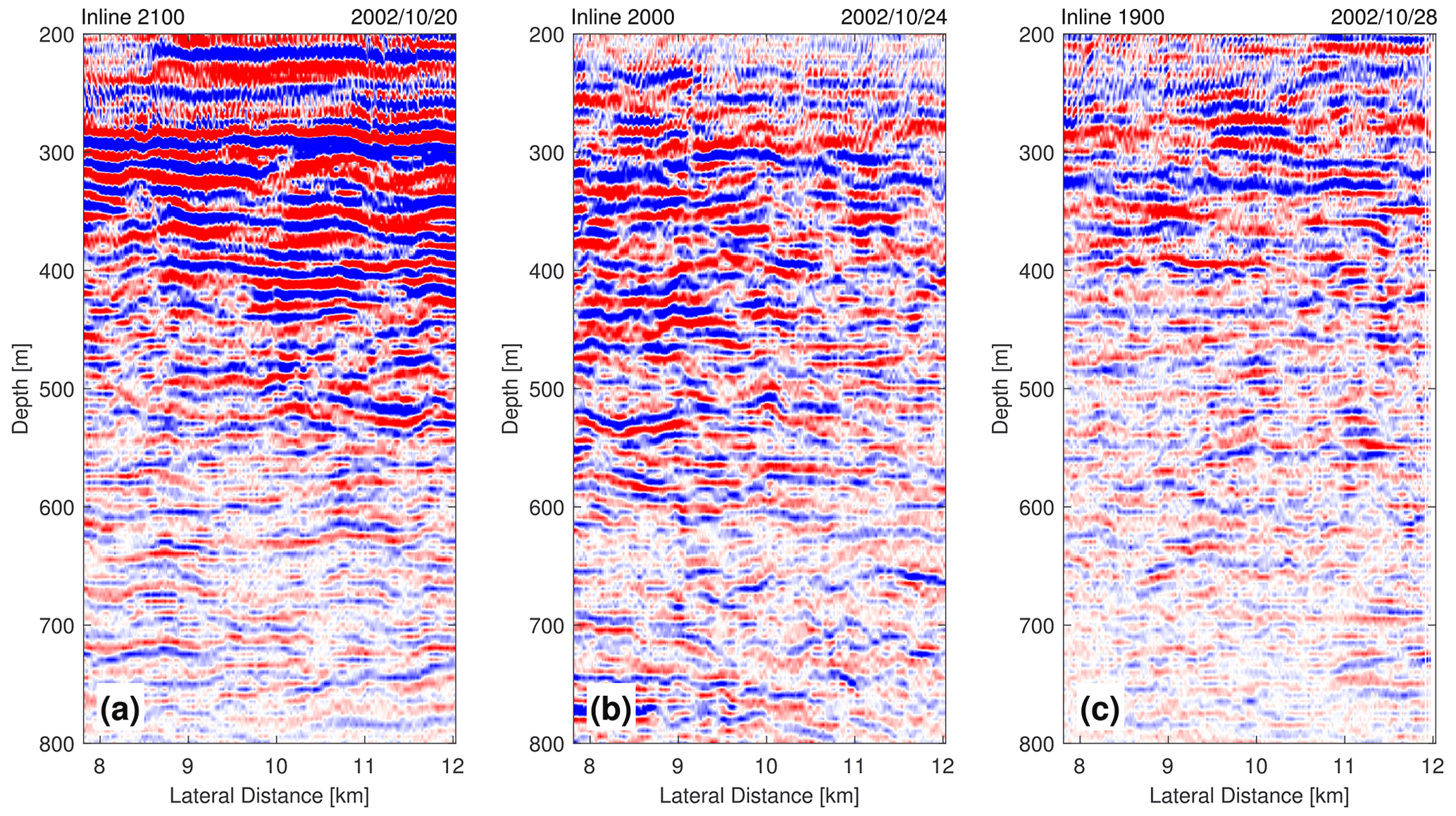
Figure 5 Three seismic inline images illustrating temporal variation of the water column. (a) IL #2100, (b) IL #2000, and (c) IL #1900. Inline numbers and the date of collection are noted on the top. The temporal and spatial separation between images is 4 d and 2.5 km, respectively.

Figure 6 shows one of the widest crossline seismic images in our seismic area. We observe significant discontinuities and a strong pattern of seismic swaths (e.g., vertical stripes). These discontinuities stem from abrupt changes of isopycnal depth (e.g., “heaving” of isopycnals) across seismic swaths, indicating the occurrence of temporal variation in the water column. In this region, the ocean dynamics that may change isopycnal depths include eddies, internal waves, internal tides, and Mississippi River outflow. Swaths collected over the linear acquisition period (marked by the red line) display some continuity, while swaths collected with longer time shifts can yield significant discontinuities. For example, seismic imaging of the contrast acquisition period (marked by the blue line) looks drastically different from its neighboring parts due to a 20 d time shift (cf. Fig. 4). We also notice that the discontinuity varies with depth. The discontinuity is more significant at 200–350 m (Fig. 6b) than at 600–750 m (Fig. 6c), suggesting that temporal variation is more significant at shallower depths. Another proof for these discontinuities indicating temporal variation is the continuous seafloor, which has no temporal variation. Our analysis suggests that temporal variation of the water column, appearing as imaging discontinuity, is significant along the crossline direction, which lowers the quality of crossline images and may further hinder their interpretation.

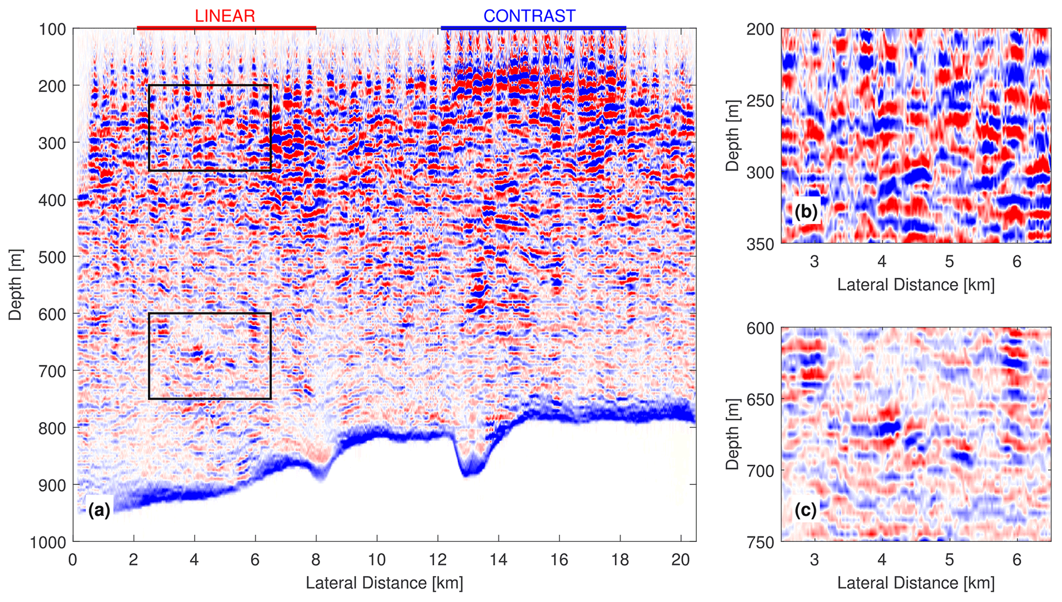
Figure 6 (a) An example of a crossline image (crossline #18200). Panels (b) and (c) are closeup views of the regions shown in (a) for two different depths. The data collection dates span from August 2002 to February 2003. The red line at top marks the linear acquisition period, while the blue line marks the contrast period.

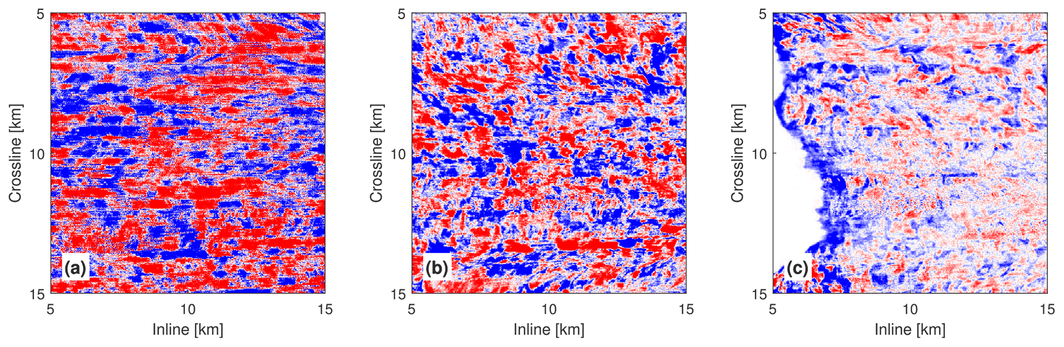
Figure 7 Seismic depth-slice images at three depths: (a) 250 m, (b) 500 m, and (c) 750 m. The two axes show the lateral distance in the inline and crossline directions, respectively.

Figure 7 shows depth-slice seismic images at three different depths (250, 500, and 750 m) to represent the shallow, middle, and deep layers of our seismic volume. Water-column seismic depth slices are the most complex representation to conceptualize since they offer a new view of the ocean interior. We observe little discontinuity along the inline direction, suggesting that temporal variation is weak along the inline direction. However, we observe a significant swath pattern and strong discontinuity appearing along the crossline direction, and the discontinuity decreases from shallow to deep layers. This decreased discontinuity agrees with the fact that temporal variability of the top ocean is more significant than that of the deep ocean, as the ocean is mainly stirred from the top due to the wind-driven surface mixing (Talley et al., 2012). Due to the presence of temporal variation, interpreting seismic depth-slice images is extremely challenging, but we may get a hint of the timescale of the ocean dynamics in Fig. 7 based on the number of discontinuities and our 3D seismic setup (e.g., time separation between nearby seismic swaths). We suggest that in this region the ocean dynamics have a timescale less than 8 h at a depth of 250 m but longer than 8 h at 750 m. The analysis of depth-slice images suggests that in our seismic volume, temporal variation of the water column is non-negligible in the crossline direction but negligible in the inline direction. In other words, temporal variability is dominant at timescales greater than a few hours.

This qualitative analysis of 3D seismic images (Figs. 5–7) reveals that temporal and spatial variations are both embedded in the 3D seismic volume and temporal variation is more significant along the crossline direction than the inline direction. Next, we will conduct two analyses to quantitatively assess temporal and spatial variations within a 3D ocean seismic volume. We conduct a simple (i.e., single frequency) theoretical and complex (i.e., multifrequency) data analysis to quantitatively assess temporal and spatial variations within a 3D ocean seismic volume.

3.2 Theoretical analysis of single-frequency spatiotemporal variations

Here we describe a theoretical example to gain insight into why temporal variation appears differently in inline and crossline directions in a typical seismic surveying setup. We assume a water column in which temporal variation occurs at one cycle per day (1 cpd, about 10⁻⁵ Hz) and spatial variation at one cycle per kilometer (10⁻³ cpm). The values here are arbitrary but can represent mesoscale oceanographic processes such as internal waves or internal tides (Talley et al., 2012) for which seismic imaging is particularly useful.

Let us consider that this water column is imaged with a typical 3D seismic survey setup, having the same field geometry of our survey and carried out swath by swath like the linear acquisition period. The vessel sails at a speed of 2 m/s, the seismic swath is 400 m wide, and the vessel can collect two swaths per day. Accounting for the two-way travel time, surveying a 1 km inline section takes

$$\begin{array}{}\text{(2)}& \mathrm{1000}\left[\mathrm{m}\right]/\mathrm{2}\left[\mathrm{m}/\mathrm{s}\right]\times \mathrm{2}\left[\mathrm{ways}\right]={\mathrm{10}}^{\mathrm{3}}\left[\mathrm{s}\right]=\mathrm{0.012}\left[\mathrm{d}\right],\end{array}$$

which is negligible considering the concerned water-column dynamics have a temporal variation of 1 cpd. However, surveying a 1 km crossline section takes

$$\begin{array}{}\text{(3)}& {\displaystyle \frac{\mathrm{1000}\left[\mathrm{m}\right]}{\mathrm{400}\left[\mathrm{m}/\mathrm{swath}\right]\times \mathrm{2}\left[\mathrm{swath}/\mathrm{d}\right]}}\times \mathrm{2}\left[\mathrm{ways}\right]=\mathrm{2.5}\left[\mathrm{d}\right],\end{array}$$

which fully covers 2.5 cycles of temporal variation of the concerned dynamics here. These numbers quantitatively illustrate how the temporal variation is not significant in inline imaging yet should be accounted for in crossline imaging when using the 3D seismic data to image mesoscale oceanographic processes.

The temporal and spatial variations are illustrated for inline and crossline directions in Fig. 8a and b, respectively. The illustration is for a survey over 1 km. The spatial variation (blue curves) is given by sin (2πkx), where k is the wavenumber in the unit of cpm (recall here that k = 10⁻³ cpm). Now, to illustrate the temporal variation along the 1 km survey distance, consider how many temporal cycles have been covered over the time duration of the survey. In the inline direction, it takes 0.012 d for a 1 km survey (see Eq. 2), corresponding to 0.012 cycles of temporal variation (recall that the temporal variation period is 1 cpd). That is $\mathrm{1.2}\times {\mathrm{10}}^{-\mathrm{5}}$ cycles of temporal variation per 1 m survey distance; effectively, it is

$$\begin{array}{}\text{(4)}& k=\mathrm{1.2}\times {\mathrm{10}}^{-\mathrm{5}}\left[\mathrm{cpm}\right].\end{array}$$

However, in the crossline direction, the corresponding numbers are 2.5 cycles of temporal variation over the temporal duration of a 1 km survey (see Eq. 3); effectively, the wavenumber is

$$\begin{array}{}\text{(5)}& k=\mathrm{2.5}\times {\mathrm{10}}^{-\mathrm{3}}\left[\mathrm{cpm}\right].\end{array}$$

Based on above the settings, the temporal (red curve), spatial (blue curve), and total (sum of both; black curve) variations along the inline and crossline directions are illustrated in Fig. 8a and b, respectively. The results show that in the inline direction (Fig. 8a), temporal variation is subtle and the total variation mostly follows spatial variation. In the crossline direction (Fig. 8b), however, temporal variation is prominent and the total variation is a fair combination of both temporal and spatial variations, with temporal variation being more noticeable. This theoretical analysis confirms that with typical 3D seismic survey setups, temporal variation of mesoscale ocean dynamics is more significant in the crossline direction. In other words, inline images mostly represent spatial variation of the water column, while the crossline images represent a combination of temporal and spatial variations of the water column.

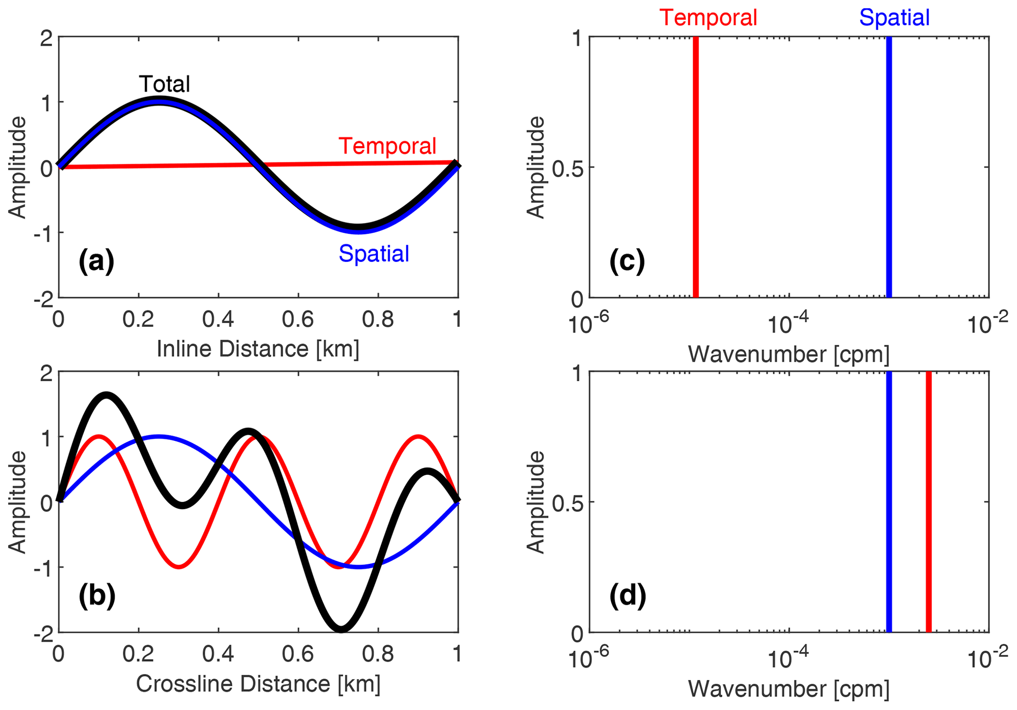
Figure 8 Illustration of temporal (red), spatial (blue), and total (black) variations in inline and crossline directions for a simple water column. (a) In the inline direction, (b) in the crossline direction, (c) spectrum of inline variation, and (d) spectrum of crossline variation. Note that the red line in (c) marked the theoretical position of temporal variations, which may not be resolved due to the short collection period. See Fig. 9a and b for further illustration of deriving inline and crossline variations from a 3D seismic volume.

Finally, Fig. 8c and d show the spectral distribution of temporal (red curve) and spatial (blue curve) components in the wavenumber domain. Here we focused on wavenumber domains instead of frequency domains because seismic images are originally intended to resolve spatial variation rather than temporal variation. In both inline and crossline directions, the spatial component appears at the same location, e.g., $k={\mathrm{10}}^{-\mathrm{3}}$ cpm, while the temporal component appears at two different locations, e.g., at $k=\mathrm{1.2}\times {\mathrm{10}}^{-\mathrm{5}}$ cpm in the inline direction (see Eq. 4) and $k=\mathrm{2.5}\times {\mathrm{10}}^{-\mathrm{3}}$ cpm in the crossline direction (see Eq. 5). In other words, in inline images, temporal variation will appear as a low-frequency component far apart (about 2 orders of magnitude, 100 times) from the spatial component, while in crossline images, temporal variation appears as a high-frequency component very close (about 2.5 times, still on the same order of magnitude) to the spatial component. The red line in the inline spectrum (Fig. 8c) illustrates the theoretical position of the temporal component, which may be too weak to resolve when inline sections are too short (i.e., covering far less than one temporal cycle). These spectral analyses suggest that water-column temporal variation will appear differently in inline and crossline images, posing strong high-frequency aliasing in the crossline imaging. Importantly, separating temporal and spatial variations in crossline imaging could be challenging because they are spectrally close to each other.

3.3 Analysis of variations in 3D seismic volume

Our theoretical analysis provides an idea for quantitatively analyzing temporal and spatial variations from the variations along the inline and crossline directions. However, real 3D ocean seismic volumes are more complicated than our single-frequency example. Here we developed a method to analyze temporal and spatial variations within our 3D seismic volume. The results will provide values of inline and crossline variations in our seismic volume, which can also be useful to other seismic oceanography studies with similar setups.

For a real 3D seismic volume, the variation along a direction can be quantified with the correlation, which measures the similarity between seismic images. The correlation for two seismic images, whose seismic amplitude stored in the 2D matrices x and y, is defined as

$$\begin{array}{}\text{(6)}& r=\sum _{i,j}{\displaystyle \frac{(x_{ij}-\stackrel{\mathrm{‾}}{x})(y_{ij}-\stackrel{\mathrm{‾}}{y})}{{\mathit{\sigma }}_x{\mathit{\sigma }}_y}},\end{array}$$

where i and j form the 2D index, $\stackrel{\mathrm{‾}}{x}$ and $\stackrel{\mathrm{‾}}{y}$ are the means, and σ_x and σ_y are standard deviations of x and y. The correlation results are between −1 and 1, representing the image similarity with respect to the reference, with +1 being exactly similar, −1 exactly reversed, and 0 completely different. In practice, the variation along the inline direction can be simply derived from the correlation between crossline images (Fig. 9a), while the variation in the crossline direction can be derived from the correlation between inline images (Fig. 9b) due to the perpendicular relationship between inline and crossline directions.

We correlate the inline and crossline image series with corresponding reference images (IL #2140, or XL #18000), respectively. The correlations are plotted as functions of inline or crossline number. The inline axis can be further converted to lateral distances (spatial domain), while the crossline axis can be converted to both lateral distances (spatial domain) and acquisition time (temporal domain). When the water-column structure varies, either temporally or spatially, the similarity between seismic images varies as well. Therefore, the change of the image similarity summarizes the variation of the water column with little change of correlation value, indicating that there has been no spatial nor temporal variations of the oceanic processes between the compared images and a big change of correlation value indicating big temporal or spatial variations.

The correlation results allow quantitative analysis of the variation of a particular image series or at a particular depth range. We only use the linear period (see Fig. 4) for a more meaningful analysis. To best represent the variation of the water column, we only use imaging of 250–750 m, excluding the seafloor and low-quality shallow portion data. Furthermore, we divide the water column into two parts, the upper part (250–500 m) and the lower part (500–750 m), to explore the depth dependency. Furthermore, the correlation function allows the examination of the correlation length, which is defined as the length to the first zero crossing, measuring the length required for two images to be completely different. The shorter the correlation length is, the faster the signal de-correlated. Finally, for periodical signals, the spectra of the correlation function can be used to study the inherent cycles within the signal.

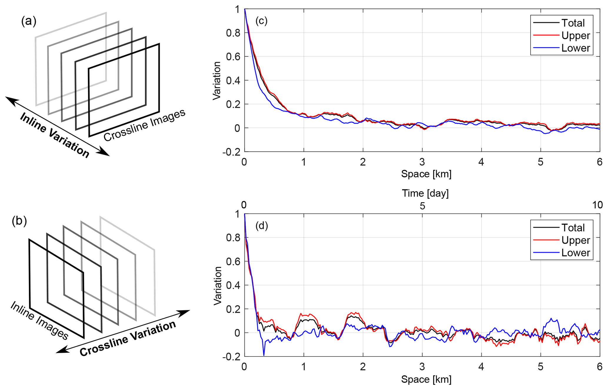
Figure 9 Inline and crossline variations from our seismic volume. Illustrations of (a) deriving inline variation from crossline image series and (b) deriving crossline variation from inline image series. Results of (c) inline variation and (d) crossline variation. The red, blue, and black curves are variations for the upper (250–500 m), lower (500–750 m), and total (250–750 m) water column, respectively. The crossline variation is calculated within the linear acquisition period (inline 1900–2140; see Fig. 4). The time and space scales in (d) follow the linear acquisition period, which spans 6 km in space or 10 d in time (yielding a ratio of 0.6 km/d). The inline variation is limited to 6 km for easy comparison with the crossline.

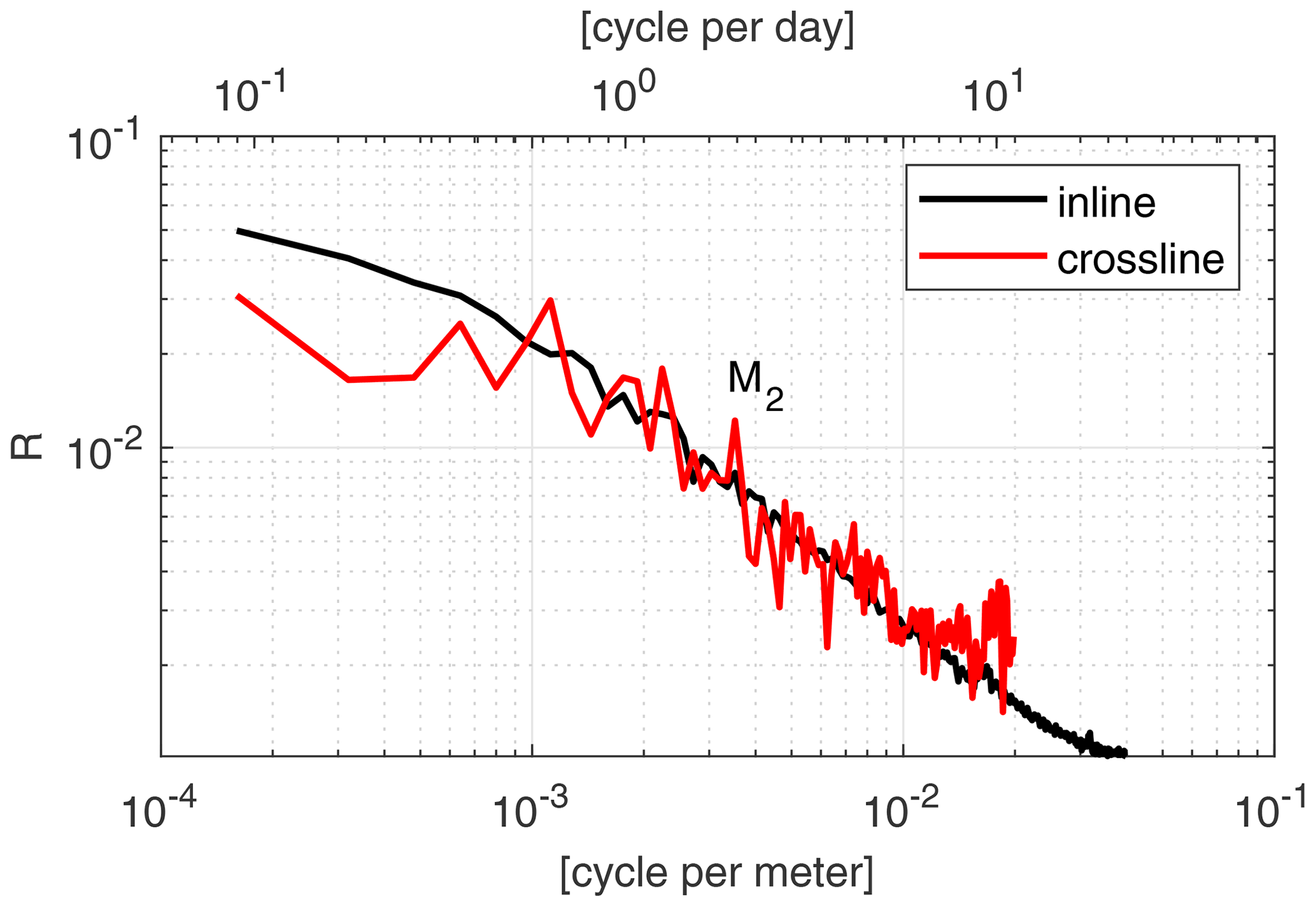
Figure 10 Inline and crossline spectra. The crossline spectrum is associated with both time and space cycles (with a ratio of 0.001666 cpm/cpd) calculated from the Fourier transform of the crossline variation in the timescale and from that in the space scales, respectively. The inline spectrum is only associated with the space cycle, calculated from the Fourier transform of the inline variation. The semi-diurnal (M₂) tidal cycle is also denoted (at 2 cpd, or about $\mathrm{3.3}\times {\mathrm{10}}^{-\mathrm{3}}$ cpm in the space scale).

Figure 9 shows the results of the variation in the inline direction (namely, inline variation) and that in the crossline direction (namely, crossline variation) derived from our 3D seismic volume. Here, inline variation (Fig. 9c) is plotted as a function of space (i.e., lateral distance), while crossline variation (Fig. 9d) is plotted as a function of space or time (based on the acquisition time). Overall, both inline and crossline variations quickly decrease from unity and then fluctuate around zero. The upper and lower water columns vary differently and the variation of the whole water column is mostly dominated by the upper part. Comparing these two directions, three observations can be made: (a) the crossline variation fluctuates more than the inline variation, (b) the crossline variation has a shorter correlation length (about 0.4 km) than the inline variation (about 2.5 km), and (c) the crossline variation has more high-frequency fluctuations than the inline variation. These observations can only be explained with the presence of temporal variation in crossline variation, leading to more and faster fluctuation and shorter correlation lengths, agreeing with our theoretical analysis (see Fig. 8a and b). Thus, our analysis confirms that in our 3D seismic volume, the inline variation (Fig. 9c) is mostly associated with spatial variation, while the crossline variation (Fig. 9d) is associated with both temporal and spatial variations.

Figure 10 shows the spectra calculated from the total variations (black curves in Fig. 9) along inline and crossline directions. Note that the inline is only associated with space, while the crossline is associated with both time and space. Overall, we observe a similar descending trend in both spectra, providing us information about the spatial features in wavenumber domains. Comparing these two spectra, one can see that the many peaks seen in the crossline spectrum are absent in the inline spectrum. These peaks show the dominant frequencies of temporal variations. Particularly, we observe the semi-diurnal tidal cycle (marked as M₂ in Fig. 10) in the crossline spectrum, which is strong evidence that the crossline variation includes temporal variations, as continental marginal waters are often heavily influenced by tidal-forcing dynamics. A significant number of high-frequency components seen in the crossline spectrum are temporal variation, agreeing with our theory (Fig. 8d), which suggests that temporal variation appears as a high-frequency aliasing. Our spectral analysis, again, confirms that the crossline imaging captures temporal features of the ocean, while the inline imaging only captures the spatial features.

4 Discussion

The visual, theoretical, and data-driven analysis of the 3D seismic volume has provided information about the way in which temporal and spatial oceanic variability is captured by 3D seismic surveys. Notice that this is a fairly new field and we do not have a complete catalog of results and detailed concurrent oceanographic measurements that would allow unambiguous interpretation of the 3D seismic imaging in light of oceanographic processes.

Fundamentally, 3D seismic oceanography resolved from common 3D seismic survey setups will be intrinsically affected by temporal variations of ocean dynamics. Ideally it is possible to design a 3D seismic survey that can perfectly image an oceanographic process without significant temporal variation. However, 3D seismic surveys are very expensive to collect and, in most cases, we have to rely on data acquired for other purposes. 3D seismic surveys conducted for oil and gas exploration cover a very large volume of ocean water and have a suitable bandwidth to depict water-column reflections. Those surveys are often acquired over time spanning days to months, and we must look for the oceanographic signals embedded in the seismic data and build the best processing and analysis workflow. Mesoscale and sub-mesoscale ocean dynamics (e.g., fronts, eddies, internal waves, and turbulence) have frequencies of 10⁻⁶–10² Hz and wavenumbers of 10⁻⁴–10² cpm (Talley et al., 2012; Ruddick, 2018). As a result, wave spectra resulting from mismatched imaging inevitably produce a significant overlap of temporal variations on top of spatial variation. Temporal variation in 3D imaging may vary case by case, dataset by dataset, and volume by volume.

Standard 3D seismic data processing for earth interior imaging utilizes reflections within a large volume of sub-seafloor to provide high-quality images and eliminate “ghost” reflections from nearby offline features that 2D processing are prone to (Yilmaz, 2001). When applying 3D processing for ocean imaging, the general rule is to avoid summing inconsistent reflections from different seismic swaths. In practice, narrow aperture 3D multiparametric stacking (Bakhtiari Rad and Macelloni, 2020) or swath-by-swath common midpoint 3D stacking (Blacic and Holbrook, 2010) can both be used to create 3D seismic oceanographic images because both implement a time-dependent selection for the seismic data. However, the processing workflow for 3D seismic oceanography can be case-dependent and we suggest always performing an in-depth temporal analysis to avoid summing time-inconsistent seismic data.

Generally, we found that:

Inline images are not affected by temporal variation unless the inline is very long or is imaging fast-moving water-column structures (Klaeschen et al., 2009). Each inline image can be seen as a snapshot of the water-column vertical thermocline structure at a given time over a given location. Therefore, available image analysis methods developed for 2D seismic oceanography, e.g., wave field spectral analysis (Holbrook et al., 2013) and diffusivity estimations (Fortin et al., 2017; Dickinson et al., 2017), can be safely extended to 3D inline images because temporal variation is small in the inline direction. Most importantly, because an inline section “samples” the ocean at one given time and one given place, we could have a particular sequence of inline images that adequately image both the spatial and temporal variations of oceanographic processes. This knowledge can be applied to understand time-evolving mesoscale ocean dynamics, e.g., eddies and internal waves, as the evolution of their vertical structures is very difficult to capture using traditional in situ oceanographic measurements. Recent 3D seismic oceanography studies with the time-lapsing concept (Dickinson et al., 2020; Gunn et al., 2020) are perfect examples of the application of this temporal variability in oceanographic studies. This temporal feature makes 3D seismic oceanography an extremely powerful tool for studying the temporal evolution of mesoscale ocean dynamics.

Crossline images capture both temporal and spatial information, and temporal variation is more prominent than spatial variation in the crossline direction. The temporal variation exhibits as a discontinuity (Fig. 6) and faster correlation fluctuations (Fig. 9) in the crossline direction. These time-related features are verified by theoretical analysis (Fig. 8b, d). In contrast, if the amplitudes of temporal variability are less than those associated with spatial variability, the temporal changes would not be apparent. For example, the seafloor appears highly continuous (does not exhibit temporal variations) in our crossline imaging (Fig. 6) because it is associated with a long geological timescale longer than years. In general, ocean crossline images appear as low-quality seismic images, which might limit the imaging interpretation. This is mostly due to discontinuity induced by temporal variation rather than fewer receivers in the crossline direction than in the inline direction (8 vs. 640). Therefore, the low quality cannot be improved through common processing techniques such as trace interpolation (Yilmaz, 2001). Instead, the crossline imaging can only be improved by optimized 3D seismic survey configurations specifically designed for seismic oceanography, e.g., faster data collection across swaths in the crossline direction. Nevertheless, crossline images still provide valuable information, offering an immediate overview of the temporal distribution of the seismic survey.

In depth-slice images, temporal variation only appears in the crossline direction and is highly depth-dependent. This depth dependency comes from the timescale of ocean dynamics that occur at different depths. Due to water mixing of surface wind waves, the top portion of the water column is usually highly dynamic, while the deep water is associated with a very long timescale (Talley et al., 2012). Such a depth dependence, in terms of imaging discontinuity, can be seen in the crossline images (Fig. 6) and depth-slice images (Fig. 7), which is also evidence of the presence of temporal variation in the crossline direction. This depth dependency in 3D seismic oceanography can be a useful indicator to study the timescale of ocean dynamics at different depths.

Our understanding of temporal and spatial variations in 3D seismic oceanography is essential for interpreting 3D seismic images. First, each inline image should be interpreted as purely spatial structures because temporal variation is insignificant in the inline direction. However, a series of 3D inline images can be interpreted as snapshots at different “moments”. The interpretation is based on the situation when multiple inline sections across the crossline direction have a survey time longer than the temporal scale of investigated ocean features, yet have a spatial scale smaller than the dimensions of the feature. Therefore, we interpret Fig. 5 as three snapshots of unique ocean thermohaline structures and internal wave fields, suggesting the weakening of thermoclines and the intensification of internal wave mixing at the continental slope of northern Gulf of Mexico during 20–28 October 2002. Second, the horizontal axis in the crossline images should be interpolated as time rather than distance because temporal variation is more significant than spatial variation in the crossline direction. In this sense, we interpret Fig. 6 as the complex temporal variation of ocean thermohalines during August 2002 to February 2003 (cf. Fig. 4). For example, during the linear acquisition period (lateral distance from 8 to 2 km, corresponding to 20–28 October 2002), the main thermoclines at the depth of 200–400 m went from stronger and thicker layers to thinner and weaker layers, suggesting the increased water mixing during this period. Third, ocean depth-slice images would be difficult to interpret. Depth-slice images provide a horizontal view of the ocean interior, which can be useful for identifying horizontal ocean features like eddies. We suggest interpreting the inline axis as horizontal distance and interpreting the crossline axis primarily as time. Unfortunately, we are unable to interpret Fig. 7 because we did not recognize obvious eddy or other horizontal ocean features in our relatively small imaging region.

Finally, based on our analyses of these 3D seismic images, we explore the possible mesoscale ocean process causing the water-column mixing during the linear acquisition period. Prior studies showed that the water dynamics in this region are dominated by the Loop Current and Mississippi River outflows, and possible ocean dynamics may include river plumes, internal waves, internal tides, and eddies (Coleman, 1988; Sturges and Lugo-Fernandez, 2005; Hamilton and Lee, 2005). The temporal and spatial variability observed from these seismic images (Figs. 5–7) suggests a mesoscale ocean process with a temporal cycle longer than 8 d (the time separation between seismic images), a length scale larger than 25 km (exceeding the maximum width of our seismic images), and a depth of influence down to 800 m (generating internal wave field near the seafloor). Cross-referencing the above scales with the typical scales of possible ocean dynamics in this region, the only matched ocean dynamics are eddies. The Loop Current creates omnipresent cyclonic and anticyclonic eddies, moving northward and eastward in the Gulf of Mexico. We suggest that our seismic images have captured the process of an eddy approaching the northern continental slope. When eddies approach the continental margin, they start to interact with the continental slope and generate internal wave fields over the slope. This process increases the vertical mixing and reduces the stratification, leading to a change of the water column from highly stratified to well mixed (as seen in Fig. 5). A full investigation of the ocean dynamics observed in our seismic images would involve concurrent in situ measurements and satellite data, which is beyond the scope of this present study and will be reported in a different paper.

5 Conclusions

This study focuses on providing a fundamental understanding of spatial and temporal variations embedded in 3D seismic data collected for oil and gas exploration. A 3D seismic volume of the northern Gulf of Mexico water column is presented, and temporal and spatial variation in 3D oceanic seismic volume are investigated for the first time using theoretical analysis and a correlation-based data analysis. Our results show that in typical 3D seismic surveys, temporal variation of mesoscale ocean dynamics can appear in the crossline direction, allowing one to view individual inline images as time-lapsing snapshots. The crossline and depth-slice images are heavily affected by temporal variation and they cannot be interpreted purely as space (i.e., distance). Instead, we suggest that they should be interpreted as time (based on the acquisition time of seismic data). This deeper understanding of the potential uses of 3D seismic surveys is essential for the interpretation and analysis of 3D oceanic seismic images. It allows the extension of previous 2D seismic oceanography analysis, such as wave spectral analysis and diffusivity estimations, to 3D inline images and the study of the evolution of time-varying mesoscale ocean dynamics. The correlation analysis proposed in this study is an effective tool to access the temporal and spatial information within the seismic volume. We suggest that it is important to analyze temporal variation within a 3D seismic volume before the interpretation of 3D seismic images and the analysis of wave fields in the seismic images. We believe 3D oil industry seismic data carry a wealth of oceanographic information, and our future 3D seismic oceanography research will focus on further investigation of the evolution of mesoscale ocean dynamics (eddies and internal waves) in the northern Gulf of Mexico.