the Creative Commons Attribution 4.0 License.
the Creative Commons Attribution 4.0 License.
 | 12 Jun 2020
Are tidal predictions a good guide to future extremes? – a critique of the Witness King Tides project
John Hunter
An analysis of the viability of the Witness King Tides project (hereafter called WKT) using data from the GESLA-2 database of quasi-global tide-gauge records is described. The results indicate regions of the world where a key criterion for a WKT project (that it be executed on a day of unusually high sea level) would likely be met (e.g. the west coast of the USA) and others where it would not (e.g. the east coast of North America). Recommendations are made both for assessments that should be made prior to a WKT project and also for an alternative to WKT projects.
- Article
(3417 KB) - Full-text XML
- BibTeX
- EndNote


This work was originally stimulated by the Witness King Tides project (hereafter called WKT), which originated in New South Wales, Australia (Watson and Frazer, 2009), and is now internationally active in a number of regions, especially the USA and Australia (King Tides Project: http://www.kingtides.net, last access: 20 November 2019). WKT is a citizen-science project designed to raise awareness of the coastal impacts of future sea-level rise and to visually document the flooding that occurs at times of unusually high sea levels during the year. One of the main activities of WKT is the collection of photographs of the shoreline at the time of annual highest astronomical tide, with the aim of indicating the flooding that may occur routinely with sea-level rise (Moftakhari et al., 2015). Such flooding, if it is of low level and only causes minor rather than major disruption or property damage, is generally referred to as “nuisance flooding” (Moftakhari et al., 2018). Participants are informed of the annual highest astronomical tide in their region for a given year and are asked to photograph their local shoreline at this time (hereafter called a WKT Day or WKT Days).
While WKT is a useful way of raising awareness of the possible impacts of a higher sea level, there is, unfortunately, no perfect way of selecting a suitable WKT Day in advance. A critical assumption of WKT is that the annual highest astronomical tide is a good proxy for the actual highest water level during the year, both in timing and height. There are two potential problems with this approach: (a) that the water level on the WKT Day may be significantly modified, particularly by storm surges, and (b) a significantly higher water level may occur at a different time of the year from the WKT Day due to the coincidence of a large positive surge and an astronomical tide that is lower than the one on the WKT Day (so the opportunity of getting more dramatic photographs at this alternative time is lost). Regarding (a), during the first WKT Day on 12 January 2009 in New South Wales, Australia, the observed maximum water level was 0.09 m below the maximum astronomical tide, presumably due to a negative storm surge (Watson and Frazer, 2009). By way of comparison, 0.09 m is roughly the global-average sea-level rise from 1970 to 2009, raising the obvious question: how well is WKT likely to demonstrate the impact of future climate change if the photographed water level may be lower than expected by an amount equivalent to about 40 years of sea-level rise? A significant negative storm surge on a WKT Day may well give the unintended message that the impact of sea-level rise is likely to be unimportant.
This study uses the Global Extreme Sea Level Analysis Version 2 (GESLA-2) database of quasi-global high-frequency (i.e. sampled at least hourly) tide-gauge records (Woodworth et al., 2017) to compare the statistics of annual maxima in the astronomical tide and in sea-level observations. The results indicate how well WKT should work at over 300 locations around the world.
It should be noted that, for some locations and some years, there are more than one astronomical tides of similar magnitude to the maximum. If the tides are predominantly semidiurnal, the largest maxima occur near the equinoxes (March and September), and if the tides are predominantly diurnal, the largest maxima occur near the solstices (June and December), e.g. see Ray and Merrifield (2019). In these cases, more than one WKT Day may be declared for that year. However, the analysis to be described here only considers the case of a single WKT Day during the year.
The GESLA-2 tide-gauge database contains 39 151 station-years of data from 1355 stations (Woodworth et al., 2017). Most of these data were sampled hourly and the remainder more frequently. GESLA-2 data are composed of two data sets: one denoted “public” (which contains data for most of the world) and the other denoted “private” (which mainly contains data for Australia). For the present analysis, these data sets were combined and were downloaded on 11 March (for the “private” data) and 19 March 2016 (for the “public” data). Individual years from the tide-gauge records were selected as follows:
-
observed heights that departed by more than 10 standard deviations from the average were rejected (this is a simple check to remove extreme outliers; in the entire GESLA-2 data set of over 300 million data points, only 190 values were rejected in this way),
-
observed heights were averaged into bins to produce hourly values (this only affected the relatively few records that were sampled more frequently than hourly),
-
years with less than 80 % of hourly values were rejected, and
-
years for which the 2-year period centred on the middle of the year had less than 80 % of hourly values were rejected (this related to the tidal analysis – see later).
After this selection process, only tide-gauge records that contained at least 20 valid years were used for the results presented here. This represented a compromise between selecting long records and many records, and it yielded data from 586 individual GESLA-2 records. Henceforth, a record (i.e. italicised) refers to an individual GESLA-2 record that contained at least 20 valid years. In some cases, more than one record occupied a given location. For example, data from the same location have sometimes been sourced from different data providers, in which case they generally cover different periods and are of different lengths; such records are therefore, to a certain extent, independent and were analysed individually. However, a significant number of records are from distinct, but relatively close, locations; this could be because the metadata from different providers may contain slightly different latitudes and longitudes for the same tide gauge or could be due to genuinely different but nearby locations in the same port. For example, of the 171 405 separation distances between the 586 records, around 180 (0.1 %) are less than 3 km. Consequently, for the maps produced in Figs. 1 to 6 and in Fig. 10, the results for some records would be obscured by the results for other nearby records. For this reason, the number of records was pruned down from 586 to 311 using the “neighbourhood” technique described in Appendix A. From each neighbourhood, the record with the most years of data was selected for display in Figs. 1 to 6 and in Fig. 10. It should be stressed that this process involves no averaging; it is simply a process of removing records that probably have less significant results (based on the fact that they are shorter) and that would otherwise obscure the results of their neighbours when plotted on a global map.
For each record (denoted by index k) and for each valid year (called here the target year; denoted by index j), the following analysis was performed.
-
A tidal analysis for 102 constituents was performed on the 2-year period centred on the target year. A 2-year analysis was performed because, for a few records, a 1-year analysis failed using 102 constituents presumably because, for some constituent pairs, the Rayleigh criterion is only just satisfied. From this analysis, tidal predictions were performed for the times of all observations during the target year.
-
For each day, two periods were defined: a civil day (denoted by the subscript c), which is the full 24 h day (defined in the local time zone, based on the longitude), and a daylight day (denoted by the subscript d), which represents the period over which a natural-light photograph may reasonably be taken and which is here (somewhat arbitrarily) defined as occupying 80 % of the time between sunrise and sunset (therefore starting at 10 % of the sunrise-to-sunset time after sunrise and ending at 10 % of the sunrise-to-sunset time before sunset). Sunrise and sunset times were calculated using the SunAzimuth program.1
-
For each record, k; each valid year, j; and each “day”, i, the following were calculated for both civil days and daylight days (noting that, due to missing data, there are missing values of i and j):
- (a)
the highest predicted tide for each day (denoted for civil days and denoted for daylight days), and
- (b)
the highest observed sea level for each day (denoted for civil days and denoted for daylight days).
- (a)
-
For each record, k, and each valid year, j, the following were performed for both civil days and daylight days:
- (a)
The day of the highest predicted tide during each valid year was calculated (denoted Ipc(j,k) for civil days and denoted Ipd(j,k) for daylight days). The highest predicted tide during each valid year is therefore given by for civil days and for daylight days.
- (b)
The day of the highest observed sea level during each valid year was calculated (denoted Ioc(j,k) for civil days and denoted Iod(j,k) for daylight days). The highest observed sea level during each valid year is therefore given by for civil days and for daylight days.
- (a)
-
The following three annual metrics were obtained for each kind of day and for each valid year:
- (a)
the annual first metric, which is the height of highest observed sea level above the observed maximum on the day of the highest predicted tide for the year, given by for civil days and for daylight days;
- (b)
the annual second metric, which is the number of days when the observed sea level ( for civil days and for daylight days) was higher than the observed maximum on the day of the highest predicted tide for the year ( for civil days and for daylight days); and
- (c)
the annual third metric, which is the height of the highest observed sea level on the day of the highest predicted tide for the year above the highest predicted tide for the year, given by for civil days and for daylight days. The third metric is essentially a measure of the residual, or storm surge, on the day of the highest predicted tide for the year.
- (a)
-
Finally, the three annual metrics (5(a) to 5(c) above) were averaged over all valid years for each record (these are here called averaged metrics) and presented on global maps in Figs. 1 to 6. The spread of the first two metrics (5(a) and 5(b) above) over the valid years are presented as complementary cumulative distribution functions (CCDFs; otherwise called “exceedance distributions”) in Figs. 7 to 9.
This resulted in three types of annual metrics and averaged metrics for each record and for each of the two kinds of day (civil days and daylight days).
It should be noted that the results presented here are based on comparisons of the observed sea level with tidal predictions derived from a 2-year period of observations which include the time of the observation. This removes signals of period longer than about 2 years and most of the effects of any vertical datum shifts in the tide-gauge records. Therefore, the results are mostly indicative of intra-annual (e.g. seasonal) deviations of observations from predictions rather than of inter-annual deviations (e.g. those due to the El Niño–Southern Oscillation) or long-term trends (e.g. sea-level rise). Inclusion of these latter effects would have required the selection of longer, and therefore fewer, tide-gauge records. Such effects would be expected to expand the regions where WKT would not perform well.
Tidal analysis and prediction broadly followed Cartwright (1985), with the tidal analysis using singular value decomposition (Press et al., 2007) for the least-squares solution. Astronomical arguments and tidal frequencies were generated by software provided by the (then) Proudman Oceanographic Laboratory (now the National Oceanography Centre, Liverpool, UK).
3.1 The averaged first metric
Figures 1 and 2 show the averaged first metric for civil days and daylight days, respectively. The figures indicate how much higher, on average, the annual maximum observed sea level is above the maximum observed on the day of the highest predicted tide for the year (the WKT Day); in other words, how much better it would have been if the WKT photography had been done on the day of the annual maximum observed sea level rather than on the WKT Day (these days only rarely coincide, as discussed in Sect. 3.4 and shown in Figs. 7 to 9). As we might expect, Figs. 1 and 2 show that there is little obvious difference between the results for civil days and daylight days. The same is true for the other two metrics (Figs. 3 to 6); therefore, for Sect. 3.4 only the results for daylight days are shown.
Figure 2 (for daylight days) provides a guide to where in the world WKT is likely to be successful (low values, light colour) and where it is not (high values, dark green). The large white and dark green circles show the locations of the records discussed in Sect. 3.4, and the white and dark green ellipses show the regions discussed in Sect. 4.
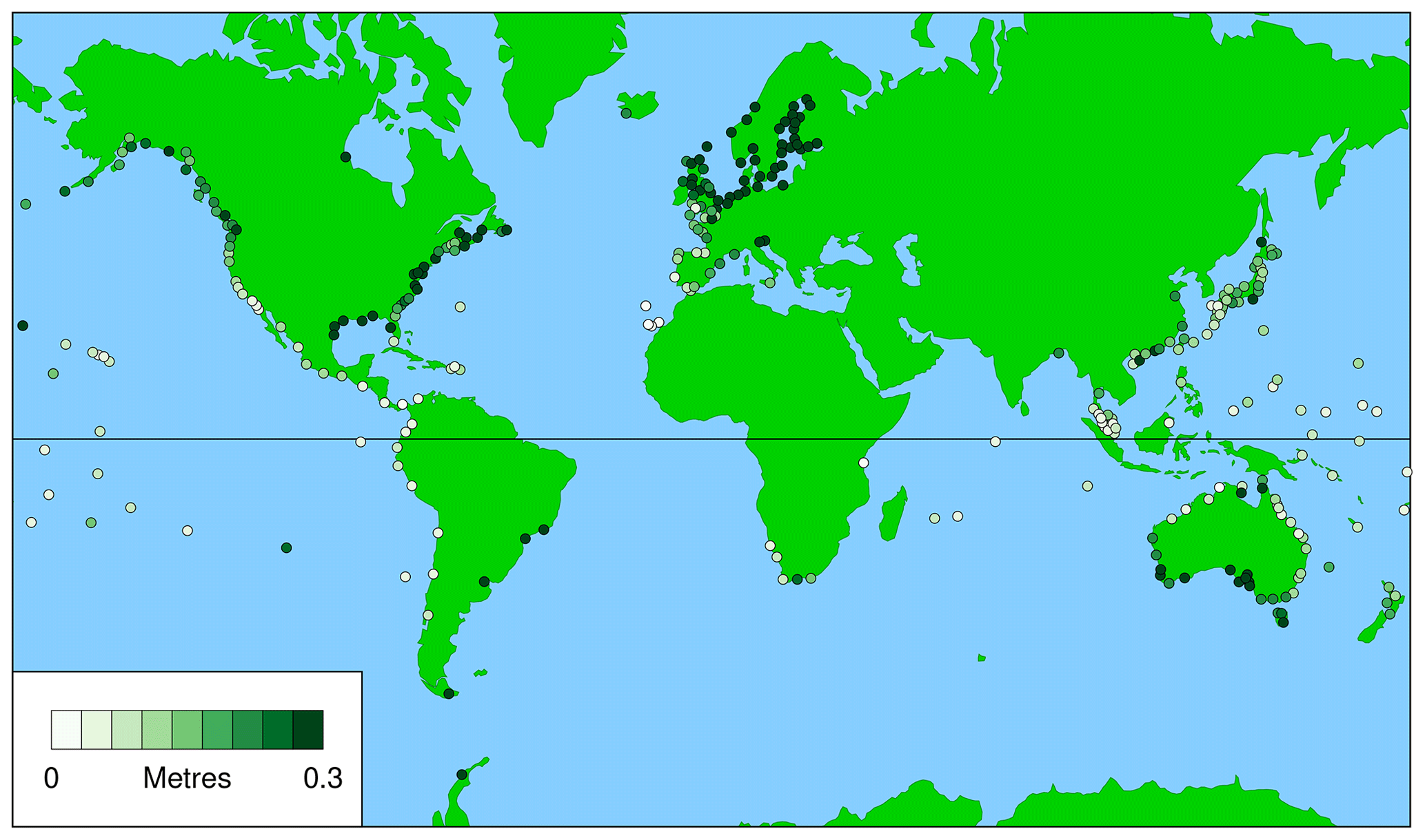
Figure 1Averaged first metric, which is height of highest observed sea level above observed maximum on day of highest predicted tide for the year, for civil days (), averaged over all valid years, j.
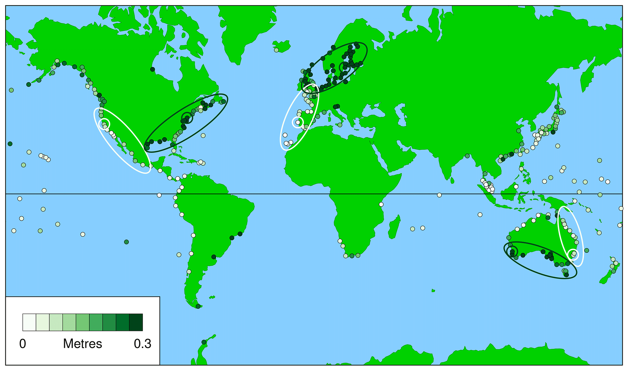
Figure 2Averaged first metric, which is height of highest observed sea level above observed maximum on day of highest predicted tide for the year, for daylight days (), averaged over all valid years, j. The large white and dark green circles indicate the records for the results shown in Figs. 7, 8, and 9. The white and dark green ellipses indicate the regions discussed in Sect. 4.
3.2 The averaged second metric
Figures 3 and 4 show the averaged second metric for civil days and daylight days, respectively. The figures indicate the number of days during the year when the sea level was higher than it was on the day of the highest predicted tide for the year (the WKT Day); in other words, how many other better opportunities there were during the year for WKT photography than on the WKT Day.
Again, the results for civil days and daylight days are very similar. Figure 4 (for daylight days) provides another guide to where in the world WKT is likely to be successful (low values, light colour) and where it is not (high values, dark green).
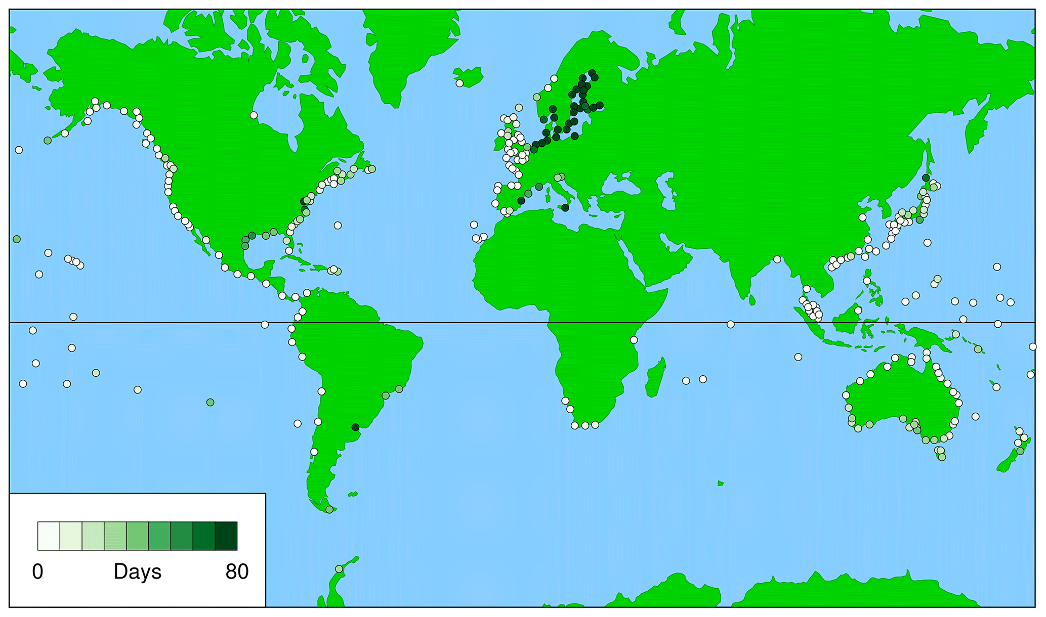
Figure 3Averaged second metric, which is no. of days when observed sea level, , higher than observed maximum on day of highest predicted tide for the year, , for civil days, averaged over all valid years, j.

Figure 4Averaged second metric, which is no. of days when observed sea level, , higher than observed maximum on day of highest predicted tide for the year, , for daylight days, averaged over all valid years, j.
3.3 The averaged third metric
Figures 5 and 6 show the averaged third metric for civil days and daylight days, respectively. The figures show the difference between the highest observed and predicted sea levels on the day of the highest predicted tide for the year, which is essentially a measure of the residual, or storm surge, on that day. This metric can have either sign (for positive or negative surges).
Again, the results for civil days and daylight days are very similar. Figure 6 (for daylight days) provides another guide to the usefulness of WKT in various parts of the world. However, in this case, the metric operates in the opposite direction to the other two. In cases where it is negative (light colour), the negative surge would clearly be problematic for WKT (it may well give the unintended message that the impact of sea-level rise is likely to be unimportant), whereas, in cases where it is positive (dark green), the positive surge could be a bonus.

Figure 5Averaged third metric, which is height of highest observed sea level on day of highest predicted tide for the year above highest predicted tide for the year, for civil days (), averaged over all valid years, j.
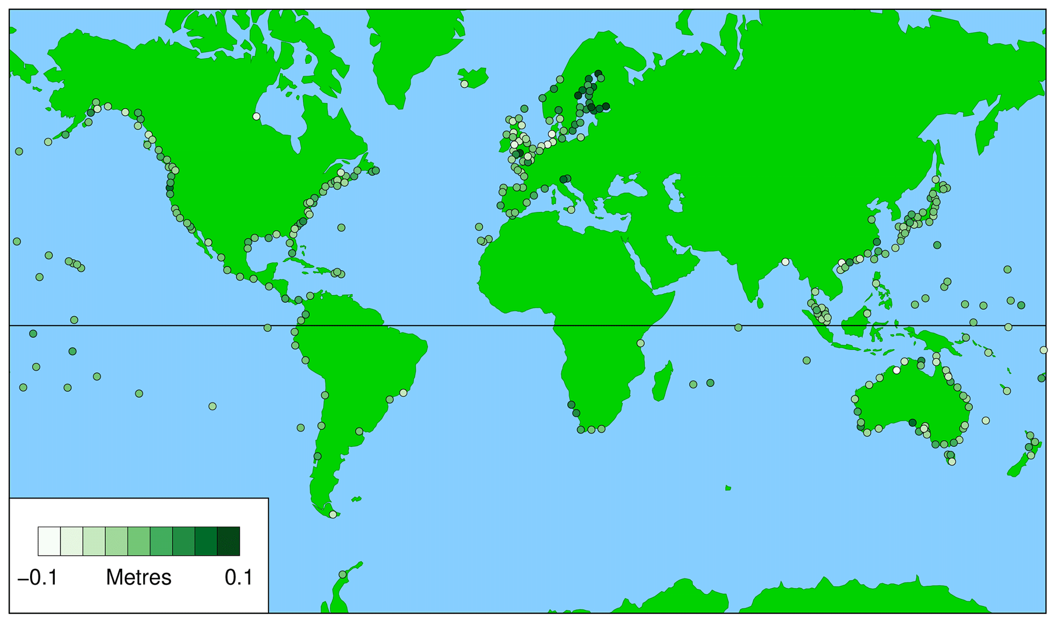
Figure 6Averaged third metric, which is height of highest observed sea level on day of highest predicted tide for the year above highest predicted tide for the year, for daylight days (), averaged over all valid years, j.
3.4 The distribution of the annual first metric and annual second metric for six typical locations on three continents
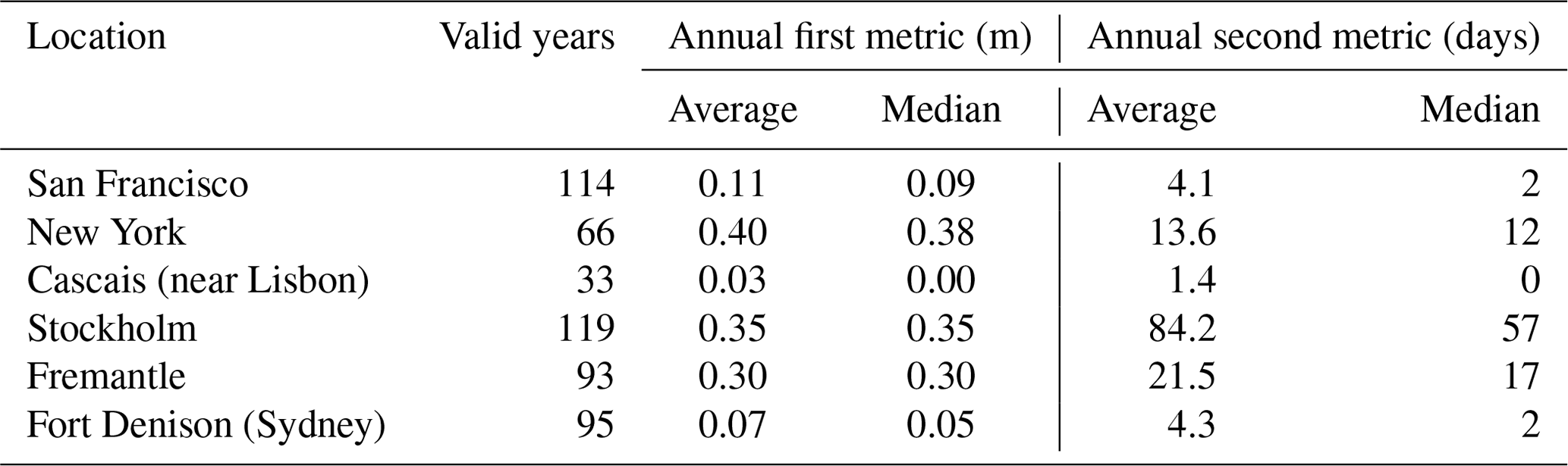
Section 3.1 to 3.3 discuss three averaged metrics derived from 311 records, which have records that contained at least 20 valid years of data and which have been pruned from the original 586 records for display on a global map. Here are presented the complementary cumulative distribution functions (CCDFs; otherwise called exceedance distributions) of the annual first metric and annual second metric for daylight days for all valid years of data for six records on three continents (San Francisco and New York in North America; Cascais (near Lisbon) and Stockholm in Europe; Fremantle and Fort Denison (Sydney) in Australia). The locations have been selected because they illustrate, within each continent, significant differences in fitness for WKT. The average and median values of these annual metrics for daylight days (i.e. those shown in Figs. 2 and 4) are shown in Table 1. The differences in fitness for WKT is evident from the significant differences of these values within each pair.
Table 1First column: location. Second column: no. of valid years in analysis. Third and fourth columns: average and median of annual first metric, which is height of highest observed sea level above observed maximum on day of highest predicted tide for the year, for daylight days (), over all valid years, j. Fifth and sixth columns: average and median of annual second metric, which is no. of days when observed sea level, , higher than observed maximum on day of highest predicted tide for the year, , for daylight days, over all valid years, j.
Two things should initially be noted about Figs. 7 to 9:
-
The intercepts on the vertical (CCDF) axes for any one location are the same for the first and second metrics. This is because years for which the annual first metric is zero are the same as the years for which the annual second metric is zero (i.e. when the highest sea level of the year occurs on the WKT Day).
-
The pairs of CCDFs all overlap to a certain extent. Therefore, although one site may perform better on average than the other site, there are always some years at the first site that are worse than some years at the other site. A measure of this overlap may be provided by the proportion of annual metric values for one site that falls within the full range of annual metric values for the other site; this is discussed for each pair of sites in the following sections.
3.4.1 San Francisco and New York
Figure 7 shows the CCDFs of the annual first metric and annual second metric for daylight days for San Francisco (one of the large white circles in Fig. 2) and New York (one of the large green circles in Fig. 2) in the USA. The CCDFs for both annual metrics are significantly narrower for San Francisco (averages of 0.11 m and 4.1 d, respectively; see Table 1) than for New York (averages of 0.40 m and 13.6 d, respectively). On this basis, San Francisco seems a better candidate for WKT than New York.
However, there is considerable variability from year to year and considerable overlap of the CCDFs for the two sites. 51 % of the annual first metric at New York falls within the full range of the annual first metric at San Francisco, while 86 % of the annual second metric at New York falls within the full range of the annual second metric at San Francisco.
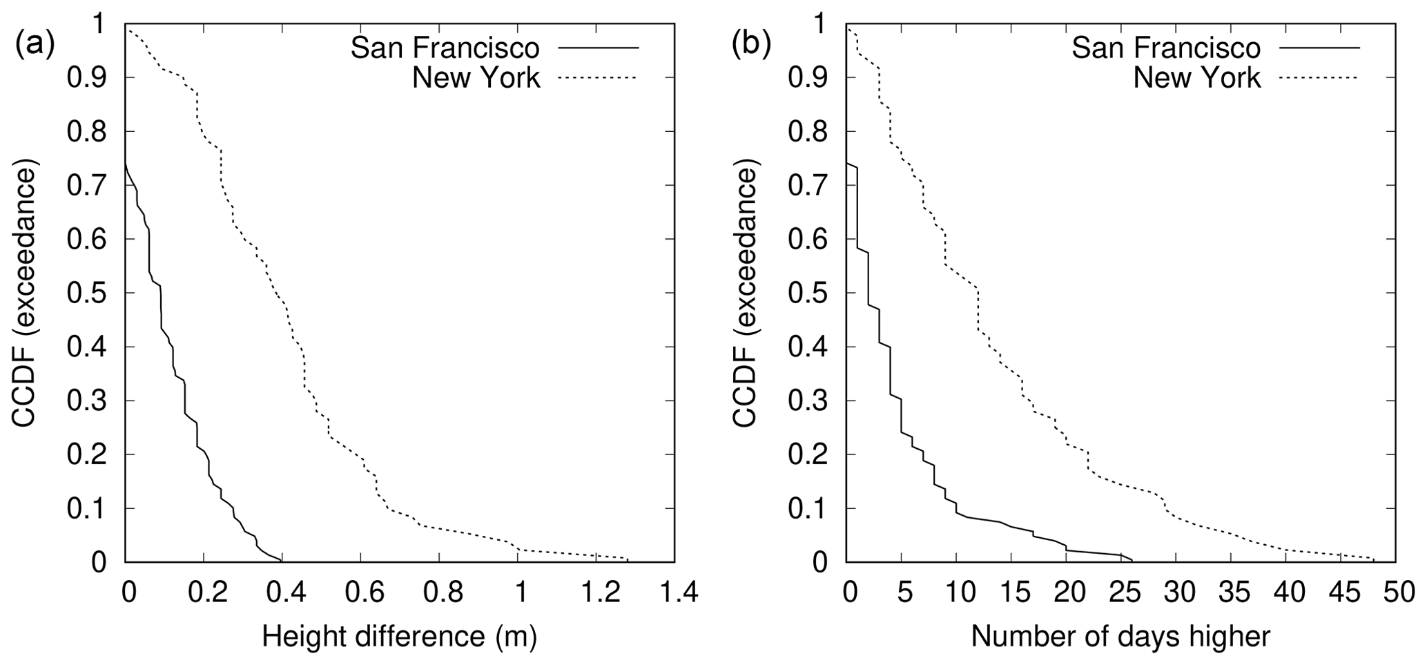
Figure 7Complementary cumulative distribution functions (CCDFs) for San Francisco and New York. (a) Annual first metric, which is height of highest observed sea level above observed maximum on day of highest predicted tide for the year, for daylight days (), estimated over all valid years, j. (b) Annual second metric, which is no. of days when observed sea level, , higher than observed maximum on day of highest predicted tide for the year, , for daylight days, estimated over all valid years, j.
3.4.2 Cascais (near Lisbon) and Stockholm
Figure 8 shows the CCDFs of the annual first metric and annual second metric for daylight days for Cascais (near Lisbon; one of the large white circles in Fig. 2) and Stockholm (one of the large green circles in Fig. 2) in Europe. The CCDFs for both annual metrics are significantly narrower for Cascais (averages of 0.03 m and 1.4 d, respectively; see Table 1) than for Stockholm (averages of 0.35 m and 84.2 d, respectively). Cascais is clearly a better candidate for WKT than Stockholm.
The contrast between Cascais and Stockholm is more marked than for the other two pairs of records, Cascais showing very narrow CCDFs, with 50 % of the annual first metric and annual second metric being zero, meaning that the highest sea level of the year occurred on the WKT Day. Only 13 % of the annual first metric at Stockholm falls within the full range of the annual first metric at Cascais, while only 7 % of the annual second metric at Stockholm falls within the full range of the annual second metric at Cascais. Cascais is clearly a good candidate for WKT.
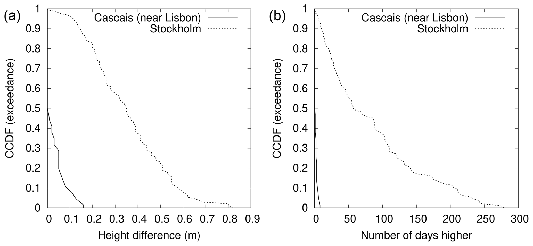
Figure 8Complementary cumulative distribution functions (CCDFs) for Cascais (near Lisbon) and Stockholm. (a) Annual first metric, which is height of highest observed sea level above observed maximum on day of highest predicted tide for the year, for daylight days (), estimated over all valid years, j. (b) Annual second metric, which is no. of days when observed sea level, , higher than observed maximum on day of highest predicted tide for the year, , for daylight days, estimated over all valid years, j.
3.4.3 Fremantle and Fort Denison (Sydney)
Figure 9 shows the CCDFs of the annual first metric and annual second metric for daylight days for Fremantle (one of the large green circles in Fig. 2) and Fort Denison (Sydney; one of the large white circles in Fig. 2) in Australia.
Qualitatively, the relationship between Fremantle and Fort Denison is similar to that between New York and San Francisco, with Fort Denison and San Francisco being the better candidates for WKT. The CCDFs for both annual metrics are significantly narrower for Fort Denison (averages of 0.07 m and 4.3 d, respectively; see Table 1) than for Fremantle (averages of 0.30 m and 21.5 d, respectively).
Again, there is considerable variability from year to year and considerable overlap of the CCDFs for the two sites: 56 % of the annual first metric at Fremantle falls within the full range of the annual first metric at Fort Denison, and 58 % of the annual second metric at Fremantle falls within the full range of the annual second metric at Fort Denison.

Figure 9Complementary cumulative distribution functions (CCDFs) for Fremantle and Fort Denison (Sydney). (a) Annual first metric, which is height of highest observed sea level above observed maximum on day of highest predicted tide for the year, for daylight days (), estimated over all valid years, j. (b) Annual second metric, which is no. of days when observed sea level, , higher than observed maximum on day of highest predicted tide for the year, , for daylight days, estimated over all valid years, j.
3.5 The variances of the observed sea level and of the predicted tide
As noted in the Introduction section, the success of WKT depends strongly on the size of the storm surge (which is indicated by the third metric, displayed in Figs. 5 and 6) relative to the tide; in general, strong storm surges confound attempts to predict the day when WKT would be successful while, if the storm surge were always zero, the WKT Day (i.e. the day with the highest predicted tide of the year) would always be the day of the highest sea level of the year. It is therefore possible that the relative magnitudes of storm surge and tide could provide a simple alternative to the metrics discussed earlier. Figure 10 shows the ratio of the variance of the observed sea level to the variance of the predicted tide (both calculated in the same way as for the derivation of the metrics, as described in the Methods section). It provides another guide to where in the world WKT is likely to be successful (low values, light colour) and where it is not (high values, dark green).
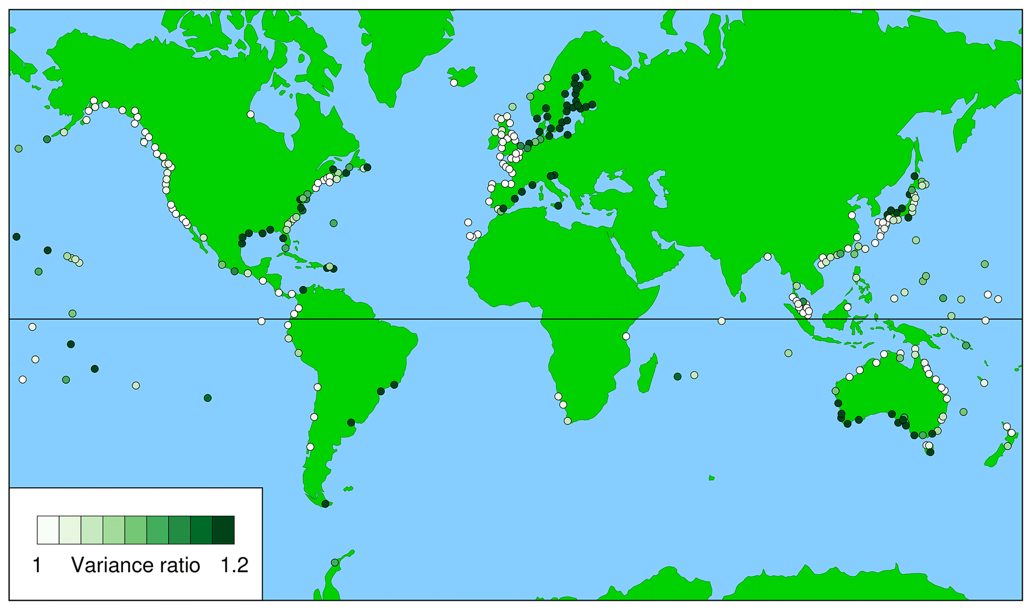
Figure 10Ratio of variance of observed sea level to variance of predicted tide.
Figures 1 to 6 provide maps showing the three metrics, averaged over at least 20 valid years for 311 tide-gauge records. The best measures for suitability for WKT are the averaged first metric and averaged second metric (Figs. 1 to 4), as they are based on observations throughout each of the years analysed. Sites where it would be expected that WKT would perform well are indicated by low values (light colour), while high values (dark green) suggest poor performance.
Less useful, though nevertheless interesting, is the third metric (Figs. 5 to 6), which shows the storm surge averaged over all WKT Days; it is less useful than the other metrics, because it is based solely on information from WKT Days. In cases where it is negative (light colour), the negative surge would clearly be problematic for WKT (it may well give the unintended message that the impact of sea-level rise is likely to be unimportant; indeed, this was a prime impetus for the present work), whereas, in cases where it is positive (dark green), the positive surge could be a bonus.
Figures 1 to 6 are presented in two ways: for civil days (i.e. the normal 24 h day) and daylight days (i.e. the periods over which a natural-light photograph may reasonably be taken). Inspection of the figures indicates that there is little difference between the results for civil days and daylight days, so the following discussion relates only to the results for daylight days.
Figure 2 (the averaged first metric for daylight days) indicates three regions where WKT should perform well (white ellipses):
-
the west coast of the USA,
-
southwestern Europe and locations off northwestern Africa, and
-
the east coast of the Australian mainland.
Figure 2 also indicates three regions where WKT should perform poorly (dark green ellipses):
-
the east coast of North America,
-
northern Europe, and
-
the south and southwest coast of the Australian mainland and Tasmania.
These regions coincide with the pairs of typical records shown in Figs. 7 to 9 and summarised in Table 1. It appears fortuitous that the first WKT project was conducted in New South Wales, which is the region around Fort Denison (Sydney), shown by the white circle in southeastern Australia in Fig. 2. The large values of the averaged first metric in northern Europe are related to a combination of weak tides (e.g. in the Baltic; Stigebrandt, 2001) and significant surges (e.g. in the North Sea; Huthnance, 1991).
Figure 4 (the averaged second metric for daylight days) shows generally the same features as Fig. 2 but the contrasts are not so marked. Low values in southwestern Europe and locations off northwestern Africa and high values in northern Europe are clear, but the variations in North America and Australia are more subtle.
Figure 10 shows an alternative estimator of the viability of WKT, which is the ratio of the variance of the observed sea level to the variance of the predicted tide (again derived from records with at least 20 years of valid data); in this case, WKT is likely to be viable at sites with a low value (light colour). Figure 10 shows many of the features displayed by the first metric for daylight days (Fig. 2), indicating that this simple estimator may be as useful as the first metric in determining regional variations in the performance of WKT.
Figures 2 and 10 provide useful preliminary indicators of regions where a WKT project may be successful, in the sense that the day of highest predicted tide for the year (the WKT Day) would yield an observed level comparable with the maximum observed level for the year. However, it is suggested that, prior to initiating a WKT project, local tide-gauge records that are longer than 20 years are analysed in ways similar to those described here (e.g. the production of figures similar to Figs. 7 to 9) to provide a more detailed assessment of the viability of WKT.
It is, however, unclear whether the WKT strategy (i.e. picking, in advance, the day when the coast is to be photographed) is the best one. An attractive alternative is to photograph every high tide of the year and pick, in retrospect, the images which show the highest sea level. This procedure could be quite easily performed using the camera of a smartphone, suitably programmed to take photographs at the required times and to transmit them to a central repository.
In order to reduce the density of the locations of records, the locations were divided into groups which are here called neighbourhoods. A neighbourhood is a unique and objectively defined group of locations in which every location is within a prescribed distance, d, of at least one other location in that neighbourhood. In a similar way to houses in a neighbourhood, a house is close to one or more of its neighbours, but not necessarily close to all the other houses in the neighbourhood. The method proceeds as follows:
-
Calculate symmetric n×n matrix Ai,j of ellipsoidal distances between all n locations.
-
For all (i,j), if , set ; otherwise, set , where d is a prescribed distance. An entry of 1 in Ai,j therefore indicates that the pair of locations are close.
-
Matrix multiply Ai,j with itself to yield another symmetric matrix, Bi,j (i.e. ), and set all finite values of Bi,j to 1 (i.e. if , then ).
-
If , set Ai,j to Bi,j and go to step 3; otherwise finish.
The resultant matrix, Bi,j, generally contains numerous repeated rows (and also columns, because Bi,j is symmetric). Bi,j may be simplified by removing any rows that are repeated, yielding a non-symmetric m×n matrix, Ci,j, where m is the number of neighbourhoods. Ci,j represents a table indicating in which neighbourhood a given location lies (the jth location lies in the ith neighbourhood if ). Each column of Ci,j contains a single 1, because a location can only lie in one neighbourhood.
The above procedure converges quickly. For d=75 km, the locations of the 586 records yielded 311 neighbourhoods and required only four iterations of steps (3) and (4).
Tide-gauge data used in these analyses were obtained from the Global Extreme Sea Level Analysis Version 2 (GESLA-2) database: https://gesla.org/ (last access: 19 March 2016), which is a slightly updated version of the database described by Woodworth et al. (2017).
The author declares that there is no conflict of interest.
This article is part of the special issue “Developments in the science and history of tides (OS/ACP/HGSS/NPG/SE inter-journal SI)”. It is not associated with a conference.
I am very grateful to Philip Woodworth for extensive discussions and collaborations concerning tides (including the development of the GESLA-1 and GESLA-2 databases) over many years.
This paper was edited by Richard Ray and reviewed by Ivan Haigh and Phil Watson.
Cartwright, D. E.: Tidal prediction and modern time scales, Int. Hydrogr. Rev., 62, 127–138, 1985. a
Huthnance, J.: Physical oceanography of the North Sea, Ocean and Shoreline Management, 16, 199–231, 1991. a
Moftakhari, H. R., AghaKouchak, A., Sanders, B. F., Feldman, D. L., Sweet, W., Matthew, R. A., and Luke, A.: Increased nuisance flooding along the coasts of the United States due to sea level rise: Past and future, Geophys. Res. Lett., 42, 9846–9852, https://doi.org/10.1002/2015GL066072, 2015. a
Moftakhari, H. R., AghaKouchak, A., Sanders, B. F., Allaire, M., and Matthew, R.: What is nuisance flooding? Defining and monitoring an emerging challenge, Water Resour. Res., 54, 4218–4227, https://doi.org/10.1029/2018WR022828, 2018. a
Press, W. H., Teukolsky, S. A., Vetterling, W. T., and Flannery, B. P.: Numerical Recipes 3rd Edition: The Art of Scientific Computing, Cambridge University Press, New York, NY, USA, 3 edn., 2007. a
Ray, R. D. and Merrifield, M. A.: The semiannual and 4.4-year modulations of extreme high tides, J. Geophys. Res.-Oceans, 124, 5907–5922, https://doi.org/10.1029/2019JC015061, 2019. a
Stigebrandt, A.: Physical oceanography of the Baltic Sea, in: A systems analysis of the Baltic Sea, edited by: Wulff, F. V., Rahm, L. A., and Larsson, P., chapter 2, 19–74, Springer, Berlin, Heidelberg, https://doi.org/10.1007/978-3-662-04453-7_2, 2001. a
Watson, P. J. and Frazer, A.: A Snapshot of Future Sea Levels: Photographing the King Tide, 12 January 2009, Department of Environment, Climate Change and Water NSW, Australia, ISBN 978 1 74232 472 2, 2009. a, b
Woodworth, P. L., Hunter, J. R., Marcos, M., Caldwell, P., Menéndez, M., and Haigh, I.: Towards a global higher-frequency sea level dataset, Geosci. Data J., 3, 50–59, https://doi.org/10.1002/gdj3.42, 2017. a, b, c
https://sidstation.loudet.org/sunazimuth-en.xhtml (last access: 27 June 2016.)