the Creative Commons Attribution 4.0 License.
the Creative Commons Attribution 4.0 License.
 | 24 Apr 2020
Mass, nutrients and dissolved organic carbon (DOC) lateral transports off northwest Africa during fall 2002 and spring 2003
Francisco Machín
Ángeles Marrero-Díaz
Ángel Rodríguez-Santana
Antonio Martínez-Marrero
Javier Arístegui
Carlos Manuel Duarte
The circulation patterns and the impact of the lateral export of nutrients and organic matter off NW Africa are examined by applying an inverse model to two hydrographic datasets gathered in fall 2002 and spring 2003. These estimates show significant changes in the circulation patterns at central levels from fall to spring, particularly in the southern boundary of the domain related to zonal shifts of the Cape Verde Frontal Zone. Southward transports at the surface and central levels at 26∘ N are 5.6±1.9 Sv in fall and increase to 6.7±1.6 Sv in spring; westward transports at 26∘ W are 6.0±1.8 Sv in fall and weaken to 4.0±1.8 Sv in spring. At 21∘ N a remarkable temporal variability is obtained, with a northward mass transport of 4.4±1.5 Sv in fall and a southward transport of 5.2±1.6 Sv in spring. At intermediate levels important spatiotemporal differences are also observed, and it must be highlighted that a northward net mass transport of 2.0±1.9 Sv is obtained in fall at both the south and north transects. The variability in the circulation patterns is also reflected in lateral transports of inorganic nutrients (SiO2, NO3, PO4) and dissolved organic carbon (DOC). Hence, in fall the area acts as a sink of inorganic nutrients and a source of DOC, while in spring it reverses to a source of inorganic nutrients and a sink of DOC. A comparison between nutrient fluxes from both in situ observations and numerical modeling output is finally addressed.
- Article
(11329 KB) - Full-text XML
- BibTeX
- EndNote


The North Atlantic subtropical gyre (NASG) is one of the most important components in the thermohaline circulation. It presents a well-known intensification in its western margin, the Gulf Stream, with maximum velocities up to 2 m s−1 (Halkin and Rossby, 1985). The currents observed in this western margin of the gyre occupy a small horizontal extension compared to that of the currents in the eastern side, resulting in an asymmetric gyre (Stramma, 1984; Tomczak and Godfrey, 2003). The low intensity of the currents at the eastern boundary made them very little studied until the 1970s, when the CINECA (Cooperative Investigations of the Northern Part of the Eastern Central Atlantic) program focused on the productive African upwelling system (Ekman, 1923; Tomczak, 1979; Hughes and Barton, 1974; Hempel, 1982). Käse and Siedler (1982) found strikingly intense currents south of the Azores connected to the Gulf Stream and suggested that part of the recirculation of the NASG occurs southward in the vicinity of the African coast. Later on, several surveys based on both in situ and remote sensing observations contributed to defining the general characteristics for the average flow of the region (Käse and Siedler, 1982; Stramma, 1984; Käse et al., 1986; Stramma and Siedler, 1988; Mittelstaedt, 1991; Zenk et al., 1991; Fiekas et al., 1992; Hernández-Guerra et al., 1993).
Most of the eastward flow from the Gulf Stream is confined to a band between the Azores and Madeira islands, recirculating southward through the Canary Islands and north of Cape Verde to become a southwestward flow (Stramma, 1984). This current system is composed of the Azores Current (AC), the Canary Current (CC), the Canary Upwelling Current (CUC), the North Equatorial Current (NEC) and the Poleward Undercurrent (PUC). The AC divides into several branches defining the boundary current system off northwest Africa. It first feeds the Iberian Current (Haynes et al., 1993), while a second significant branch enters the Mediterranean Sea (Candela, 2001). Most of the AC recirculates southward, splitting into the main CC across the Canarian archipelago and the secondary CUC (Pelegrí et al., 2005, 2006). These currents extend southward, developing the Cape Verde Frontal Zone (CVFZ), a density-compensated front with North Atlantic Central Water at its northern side and South Atlantic Central Water at its southern one (Zenk et al., 1991; Martínez-Marrero et al., 2008). Finally, the PUC is located below the CUC, flowing northward on the continental slope (Barton, 1989; Machín and Pelegrí, 2009; Machín et al., 2010; Pelegrí and Peña-Izquierdo, 2015).
Mesoscale activity constitutes a second main feature in the area of interest, which might be even more energetic than the average flow itself (Sangrà et al., 2009). Three mesoscale domains may be defined: the Canary Eddy Corridor (CEC; Sangrà et al., 2009), the CVFZ and the upwelling front. The CEC is located downstream of the Canary Islands where the interaction between the southward flow and the archipelago generates long-lived eddies (Arístegui et al., 1994; Barton et al., 1998; Sangrà et al., 2007, 2009; Ruiz et al., 2014; Barceló-Llull et al., 2017a). The second mesoscale domain is the CVFZ, where several meanders and eddies produce strong interleaving between the water masses involved (Pérez-Rodríguez et al., 2001; Martínez-Marrero et al., 2008). In this domain, the CC and the CUC separate from the African coast, fueling the NEC and giving rise to a shadow zone featured by poorly ventilated waters (Luyten et al., 1983). The third area is the front arising between the coastal upwelled waters and the stratified interior waters, defining the Eastern Boundary Upwelling System (EBUS) in the northwest African region (Mittelstaedt, 1983; Pastor et al., 2008; Arístegui et al., 2009). This EBUS is actually located off the African slope from the Gulf of Cádiz until Cape Blanc–Cape Verde in summer–winter with high mesoscale variability in the form of both filaments and eddies (Hagen, 2001; Sangrà et al., 2009; Ruiz et al., 2014). The upwelling process raises nutrient-rich waters to the euphotic layer, developing a high-primary-production latitudinal band off northwest Africa known as the Coastal Transition Zone (CTZ) (Barton et al., 1998; Pelegrí et al., 2006). These mesoscale features play an essential role as a lateral source of organic matter towards the oligotrophic waters of the NASG (Barton et al., 1998; García-Muñoz et al., 2004, 2005; Pelegrí et al., 2006; Álvarez-Salgado et al., 2007; Sangrà et al., 2009).
The distribution of inorganic nutrients and organic matter in the ocean responds to a combined effect of physical and biogeochemical processes. Within the euphotic zone, primary production is solely limited by the availability of inorganic nutrients (INs) (Copin-Montegut and Copin-Montegut, 1983; Falkowski et al., 1998). Below the euphotic zone respiration exceeds primary production. As a result, the organic matter produced at the sea surface is remineralized in the subsurface layers, and hence the concentration of INs increases from the interplay between the local rate of remineralization and the rate of water supply (Azam, 1998; Del Giorgio and Duarte, 2002; Pelegrí et al., 2006; Pelegrí and Benazzouz, 2015b).
In order to study the impact of lateral transports on the distributions of biogeochemical variables, the first step to follow is to analyze the dynamic of the area with an inverse box model. This method provides a velocity field consistent with both mass and property conservation within a closed volume and with the thermal wind equation (Wunsch, 1996). Several authors have already described the circulation patterns of the NASG by applying an inverse model (Ganachaud and Wunsch, 2002; Ganachaud, 2003b, a; Hernández-Guerra et al., 2005, 2017; Machín et al., 2006; Pérez-Hernández et al., 2013). Moreover, some recent papers addressing lateral advective transports of biogeochemical variables have shed light on this topic in the EBUS off NW Africa (Álvarez and Álvarez-Salgado, 2009; Alonso-González et al., 2009; Santana-Falcón et al., 2017; Fernández-Castro et al., 2018).
To sum up, the main goal of this paper is to present an in situ hydrographic database and to estimate lateral mass as well as IN and DOC transports during fall and spring seasons south of the Canary Islands in the context of a highly variable environment featured by the Canary Eddy Corridor, the upwelling off northwest Africa and the CVFZ. The remainder of this paper is organized as follows: the dataset is presented in Sect. 2; the seasonal distribution of the water masses and their properties is displayed in Sect. 3; the technical details of the inverse box model are covered in Sect. 4; and the resulting velocity field and the corresponding mass, nutrient and organic matter transports are presented in Sect. 5. Section 6 is devoted to the discussion, with some conclusions in Sect. 7.
The COCA-I and COCA-II cruises were carried out in fall (10 September to 1 October 2002) and spring (21 May to 7 June 2003), respectively, aboard the BIO Hesperides as part of the research project Coastal-Ocean Carbon Exchange in the Canary Region (Hernández-León et al., 2019). The location of conductivity–temperature–depth (CTD), inorganic nutrient (IN) and dissolved organic carbon (DOC) stations in COCA-I and COCA-II defines a closed box along three transects (Fig. 1). The northern transect (N) spans from station 1 to 32 at 26∘ N (the section from stations 1 to 11 is tilted some 30∘ with respect to the east). The western transect (W) is located at 26∘ W from station 32 to 42. Finally, the southern zonal transect (S) at 21∘ N runs from station 42 to 63 (COCA-I) or 66 (COCA-II) over the continental slope (Table 1). The distance between neighboring CTD stations was some 50 km except for the stations over the continental slope where this distance was shortened. Adjacent DOC and IN stations were separated by a variable distance, with the shortest distance being about 50 km at stations closer to the coast.
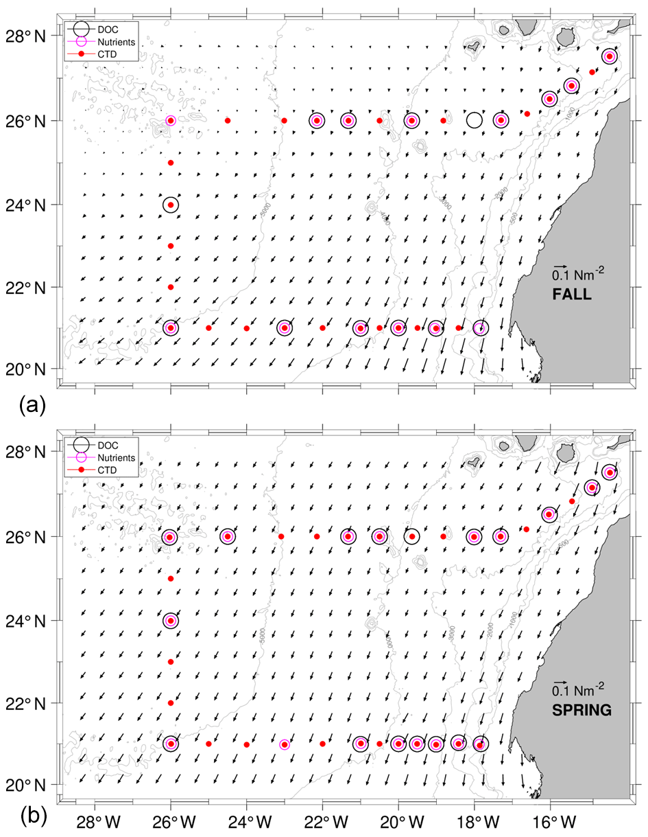
Figure 1Hydrological (red dots), inorganic nutrient (pink circles) and DOC (black circles) sampling stations during the COCA-I (a) and COCA-II (b) cruises. Time-averaged wind stress during each cruise is also represented by the inset arrow denoting the scale (shown with half of the original spatial resolution).
Table 1Summary of the number and type of measurements at stations per transect and season.
CTD data were collected from the sea surface down to 2000 m of depth with a vertical resolution of 2 dbar. In situ temperature was calibrated with 45 readings performed with a reversible digital thermometer, while salinity was calibrated by analyzing 60 water samples with the Portasal salinometer. The residuals have an average value of 0.00013±0.00400 ∘C and 0.0005±0.005 in salinity.
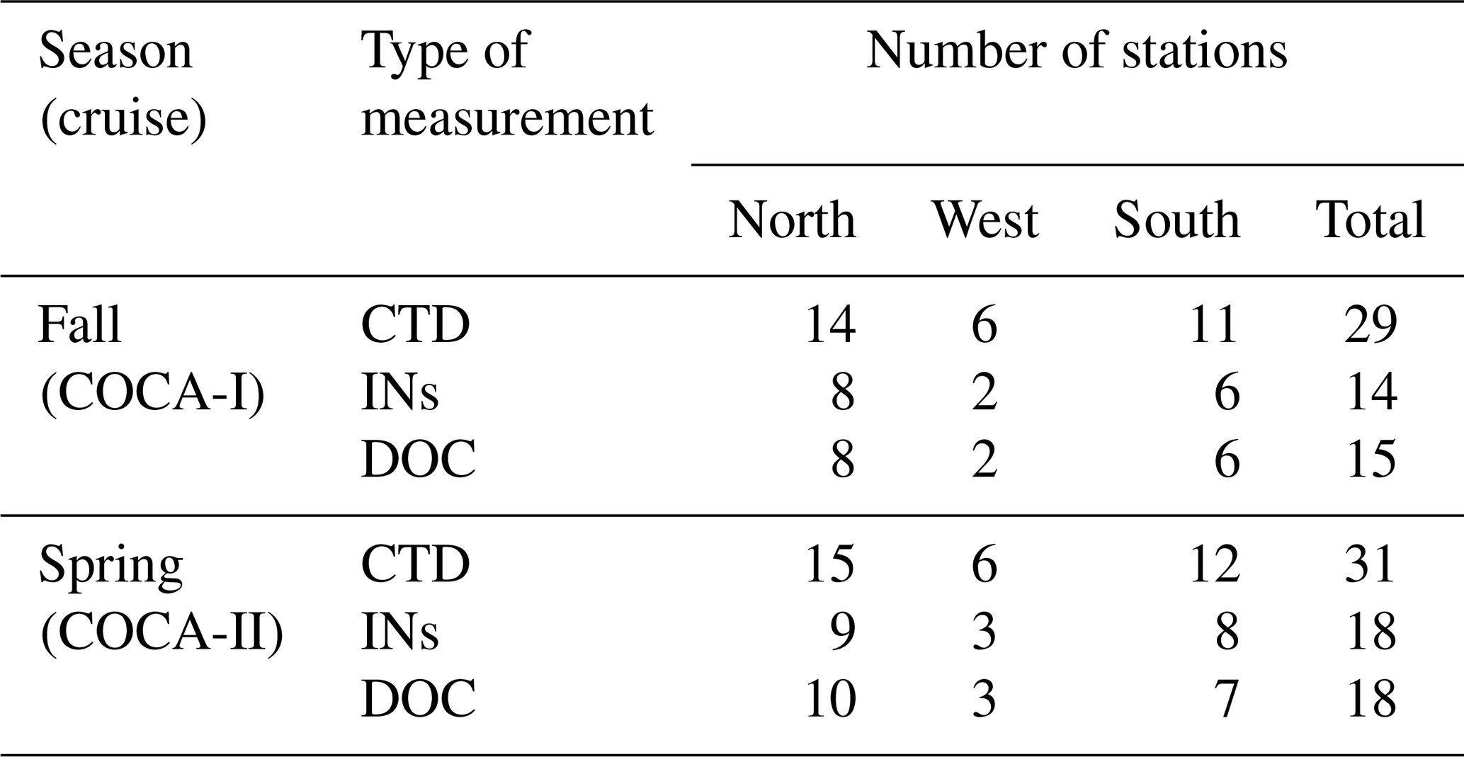
DOC was measured with a total organic carbon (TOC) analyzer (Shimadzu TOC-5000), assuming that almost all TOC was in dissolved form. Water samples (10 mL) were dispensed directly into glass ampoules previously combusted at 500 ∘C during 12 h; 50 µL of H3PO4 was immediately added to the sample, sealed and stored at 4 ∘C until analyzed. Before the analysis, samples were sparged with CO2-free air for several minutes to remove inorganic carbon. TOC concentrations were determined from standard curves (30 to 200 µM) of potassium hydrogen phthalate produced every day (Thomas et al., 1995). To check accuracy and precision, reference material from the Jonathan H. Sharp laboratory (University of Delaware) was analyzed daily. DOC distribution up to 2000 m of depth presented more representative coverage in fall than in spring (Fig. 2, green dots), despite the number of stations being higher in spring than in fall (Fig. 1, black circles; Table 1).
The three inorganic nutrients sampled were silicates (SiO2), nitrates plus nitrites (NOx) and phosphates (PO4). These samples were frozen until measured with a Bran+Luebbe AA3 autoanalyzer following the standard methodology established by Hansen and Koroleff (1999). Nutrient data covered up to 2000 m, while in fall they concentrated in the shallowest layers (<200 m; Fig. 2, pink crosses).
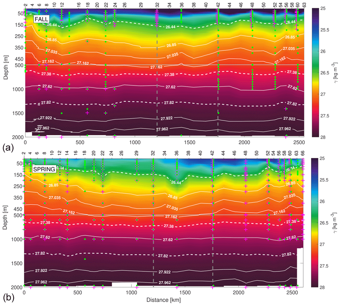
Figure 2The γn vertical sections during fall (a) and spring (b) cruises. White dashed isoneutrals limit the different water type layers. The direction chosen for the representation of the transects is the course of the vessel. Distance is calculated with respect to the first station (2). The section is divided into three transects: the northern transect from east to west (from station 2 to 32), the western transect from north to south (from station 32 to 42) and the southern transect from west to east (from stations 42 to 63–66). The three transects are separated by two vertical grey dashed lines located at stations 32 and 42. The sampling points of INs and DOC used in this work are also represented by pink crosses and green dots, respectively.
Wind data were selected from the QuikSCAT database made available by CERSAT (Centre ERS d' Archivage et de Traitement; http://www.ifremer.fr/cersat/ (last access: 20 December 2017). These wind fields were averaged weekly with a spatial resolution of 0.5∘ (shown in Fig. 1 with half of the original spatial resolution). The Smith–Sandwell database with 1 min horizontal resolution was used as the source of bathymetry data (Smith and Sandwell, 1997).
Freshwater flux data were estimated from the rates of evaporation and precipitation extracted from the Surface Marine Data 1994 of da Silva et al. (1994) (http://iridl.ldeo.columbia.edu/SOURCES/.DASILVA/.SMD94/, last access: 20 December 2017). The climatological mean depths of the neutral density field for the years 2002 and 2003 were calculated from the climatological temperature and salinity extracted from the World Ocean Atlas 2013 (WOA13; https://www.nodc.noaa.gov/OC5/woa13/woa13data.html, last access: 1 February 2018, Locarnini et al., 2013; Zweng et al., 2013).
GLORYS (GLOBAL_REANALYSIS_PHY_001_025 product) issued by the Copernicus Marine Environment Monitoring Service (CMEMS; http://marine.copernicus.eu, last access: 5 June 2018, Garric and Parent, 2018) was used as a primary source of dynamic variables. Its horizontal resolution is 1∕12∘ with 50 standard depths. Hydrological data from GLORYS were also employed to diagnose the average oceanographic conditions during each cruise. This product assimilates field observations in real time.
The SEALEVEL_GLO_PHY_L4_REP_OBSERVATIONS_008_047 product provided surface geostrophic currents estimated from sea level anomalies. These data capture the mesoscale structures and are helpful to validate the near-surface geostrophic field estimated from the inverse model.
GLORYS-BIO (GLOBAL_REANALYSIS_BIO_001_029 product) produced daily mean 3D biogeochemical fields with the same resolution as GLORYS. This reanalysis forces the biogeochemical model with the nutrient initial conditions from WOA13. IN concentrations from GLORYS-BIO (SiO2, NO3, and PO4) were used to assess nutrient transports by the model (in Sect. 5).
The data treatment, the graphical representations and the inverse model are coded in MATLAB (MATLAB, 2018). The vertical sections are produced using the “nearest” 2D interpolations, a method also employed in the estimates of the IN and DOC transports. Ocean Data View using the DIVA gridding method is employed to produce DOC concentration charts (Schlitzer, 2019).
Neutral density is used as the density reference variable, with the isoneutrals representing the surfaces where the values of γn are constant (Jackett and McDougall, 1997). The γn vertical sections contain the surface (SW), central (CW), intermediate (IW) and deepwater (DW) masses according to Macdonald (1998) for the North Atlantic at 24∘ N, represented with white dashed lines at 26.44, 27.38 and 27.82 kg m−3 (Fig. 2). The x-axis direction is selected according to the path followed by the vessel during both cruises, starting in the northeast and finishing in the southeast of the domain. The N–W and W–S corners are indicated with two vertical grey dashed lines at stations 32 and 42, respectively.
The Θ−SA diagrams exhibit four regions delimited by potential density anomaly contours of 26.39, 27.30 and 27.72 kg m−3, equivalent to the isoneutrals that separate the main water masses (Fig. 3). These three isoneutrals are approximately at 132–123, 672–700 and 1294–1305 m of depth (Fig. 2). The water masses sampled during both cruises are North Atlantic Central Water (NACW), South Atlantic Central Water (SACW), Antarctic Intermediate Water (AAIW), Mediterranean Water (MW) and North Atlantic Deep Water (NADW) (Emery and Meincke, 1986; Macdonald, 1998; Emery, 2001). Their main hydrological characteristics are summarized in Table 2. Below the mixing layer and above 700 m ( kg m−3), NACW and SACW are the dominant water masses. SACW is featured by a higher amount of nutrients, and it is 1–2 ∘C colder and 0.1–0.4 fresher than NACW (Fig. 3 and Table 2). Below, from 700 up to 1300 m ( kg m−3), the intermediate waters AAIW and MW are the dominant water masses (Hernández-Guerra et al., 2017). MW is a relatively warm and salty water mass, while AAIW is colder and fresher (Table 2). Finally, below 1300 m (γn>27.82 kg m−3) the predominant water mass is NADW, with in situ temperature and salinity values lower than 5.7 ∘C and 35.14 (Table 2).
Figure 3Θ−SA diagrams of hydrological measurements during the fall (a) and spring (b) cruises. The different water masses at the north (N, magenta dots), west (W, dark grey dots) and south (S, blue dots) transects are SW, NACW, SACW, AAIW, MW and NADW. Potential density anomaly contours equivalent to the 26.44, 27.38 and 27.82 kg m−3 isoneutrals delimit the surface, central, intermediate and deepwater levels.
Table 2Summary of water levels (CW, IW and DW) with their isoneutral limits and their water mass properties for both seasons from the sea surface to 2000 m. The properties extracted from observations are in situ temperature (T), potential temperature (θ), conservative temperature (Θ), practical salinity (SP), absolute salinity (SA) and dissolved organic carbon (DOC). The INs extracted from GLORYS-BIO are silicates (SiO2), nitrates (NO3) and phosphates (PO4).
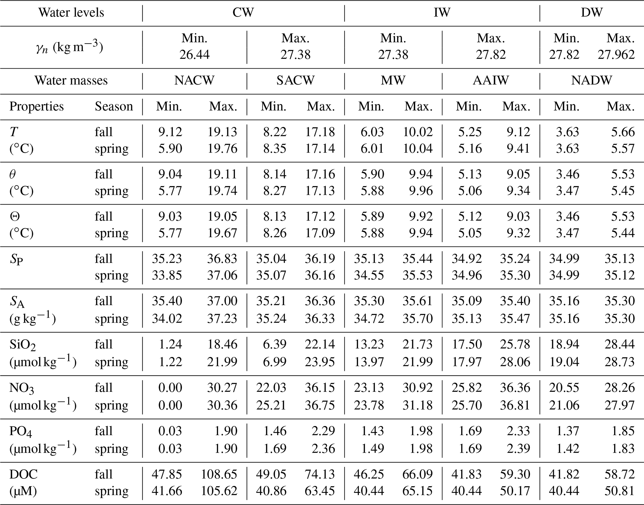
A description of the temporal variability of the water masses is also given with observations from the Θ−SA diagrams (Fig. 3). The distribution of water masses is quite similar for both cruises. There is a higher temperature variability at the surface waters during fall, with maximum values 2–3 ∘C higher than in spring. During spring, the variability observed at central waters is associated with larger fluctuations in salinity affecting the whole water column. At DW there is a higher contribution of NADW in the whole domain during fall. Finally, the surface layer is thicker in fall than in spring in all the sections made with respect to γn.
These temporal differences may also be described transect to transect. The northern transect (Fig. 2, stations 2 to 32; Fig. 3, magenta dots) is occupied by NACW, AAIW, MW and NADW in both seasons. At intermediate levels, a higher contribution of MW is observed in spring, while a slightly higher contribution of AAIW is obtained in fall. The western transect (Fig. 2, stations 32 to 42; Fig. 3, dark grey dots) has a similar distribution as the northern one, with a lower variability in the upper layers and a smaller influence of MW. In the southern transect (Fig. 2, stations 42 to 63–66; Fig. 3, blue dots), the highest spatiotemporal variability is observed. This variability at the surface and central levels is associated with the position of the CVFZ and, in turn, with the mesoscale and submesoscale structures associated with the front. The CVFZ is located where the isohaline of 36, or equivalently SA=36.15 g kg−1, intersects the 150 m isobath (Zenk et al., 1991) (Fig. 4). CVFZ is found in the southern transect in its westernmost position in fall, at stations 46–48. Hence, SACW with relatively low SA is observed above the upper limit of CW east of the CVFZ location (Fig. 4). In spring, the CVFZ shifts to a position closer to the African coast at station 52, with a water incursion of higher-salinity NACW centered at station 58 (Figs. 4 and 5). At intermediate levels, MW is registered at the northern transect, while in the southern one the predominant water mass is AAIW. Regarding the seasonal variability, the contribution of MW in the northern transect is higher in spring, while the contribution of AAIW in the southern transect is higher in fall.

Figure 4Sections of absolute salinity (SA) with respect to depth (a) and γn (b) during fall and spring. In the depth section in panel (a), the isoneutrals that delimit the transports at the surface, central, intermediate and deep water are represented by white dashed contours. In the γn section (b), the depths of 150, 672–700 and 1294–1305 m are also shown.
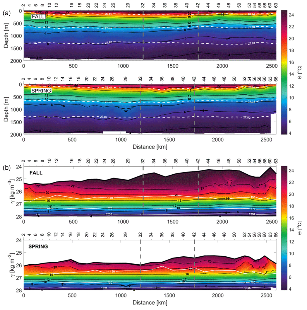
Figure 5Sections of conservative temperature (Θ) with respect to depth (top) and γn (bottom) during fall and spring. In the depth section in panel (a), the isoneutrals that delimit the transports at the surface, central, intermediate and deep water in the water column are represented by white dashed contours. In the γn section (b), the depths of 150, 672–700 and 1294–1305 m are indicated.
Although the INs have been extracted from the model and the distributions of Θ, SA and γn have been obtained from the hydrographic observations, there is a good agreement between the structures described by both datasets. The in situ concentrations of SiO2, NOx and PO4 up to 250 m of depth (black dots in Fig. 6) are represented together with the time-averaged concentrations of SiO2, NO3 and PO4 up to 2000 m of depth selected from GLORYS-BIO. In this way the IN outputs from the model are compared with in situ observations since their concentration in both cases presents an acceptable match, with the exception of NOx and PO4 concentrations at the S transect. On the other hand, the IN model outputs look like INs from historical in situ databases (not shown here).
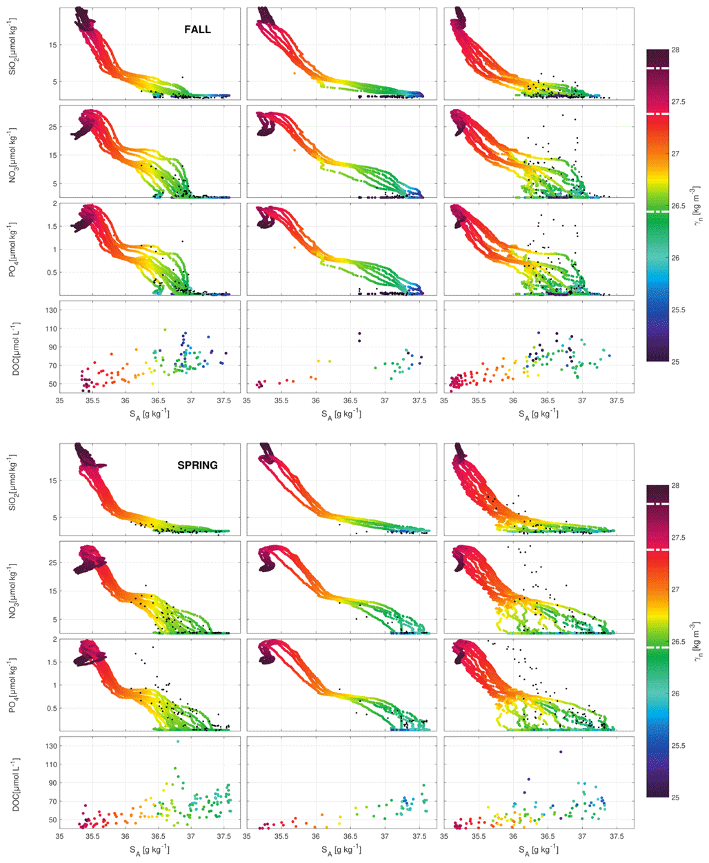
Figure 6Scatter plots for SiO2, NO3 and PO4 nutrients (µmol kg−1; extracted from GLORYS-BIO), as well as for DOC (observational data: µmol L−1) with respect to SA and γn at the north (left), west (middle) and south transects (right) in fall (top) and spring (bottom). The isoneutrals 26.44, 27.38 and 27.82 kg m−3 that limit the waters layers are indicated with white dashed lines in the color bar. The measured IN concentrations (µmol kg−1) for SiO2, NOx and PO4 until 250 m of depth are included as black dots.
At central levels, high IN concentrations have been sampled near the continental slope in both the northern (stations 10 to 18) and southern (50 to 56) transects in fall. The values observed are 1–5 µmol kg−1 for NO3 and 0.1–0.4 µmol kg−1 for PO4, which are higher values than those recorded in spring at similar places (Fig. 7). This might be related to long-lived mesoscale eddies or instabilities related to the CVFZ (Zenk et al., 1991; Sangrà et al., 2009). IN concentrations are notably high at intermediate and deep levels compared to those at central levels (Fig. 6) and have the same order of magnitude as those documented before in the domain (Pérez et al., 2001; Pérez-Hernández et al., 2013). The distributions of SiO2, NO3 and PO4 are similar during both cruises, and their concentrations increase with depth as a result of the remineralization of organic matter (Fig. 7). The area where the least nutrients are found at depth throughout the domain is the northwest corner of the box (stations 24 to 32). With respect to the IN seasonal variability at intermediate depths, the three concentrations do not present large differences between the values measured in fall and spring (Figs. 7 and 3). In both seasons the concentrations of SiO2, NO3 and PO4 are 4–6, 2–6 and 0.2–0.4 µmol kg−1 higher in AAIW than in MW (Table 2). The NADW is characterized by a moderate increase in SiO2 and a slight decrease in NO3 and PO4 with respect to the values documented here at intermediate levels. In both seasons, the maximum concentration of SiO2 is 28–29 µmol kg−1. Nevertheless, specifically in spring, the maximum concentrations of NO3 and PO4, 28 and 1.8–1.9 µmol kg−1, are lower than those recorded at intermediate levels, providing a similar vertical variability as that reported by Machín et al. (2006) (Table 2).
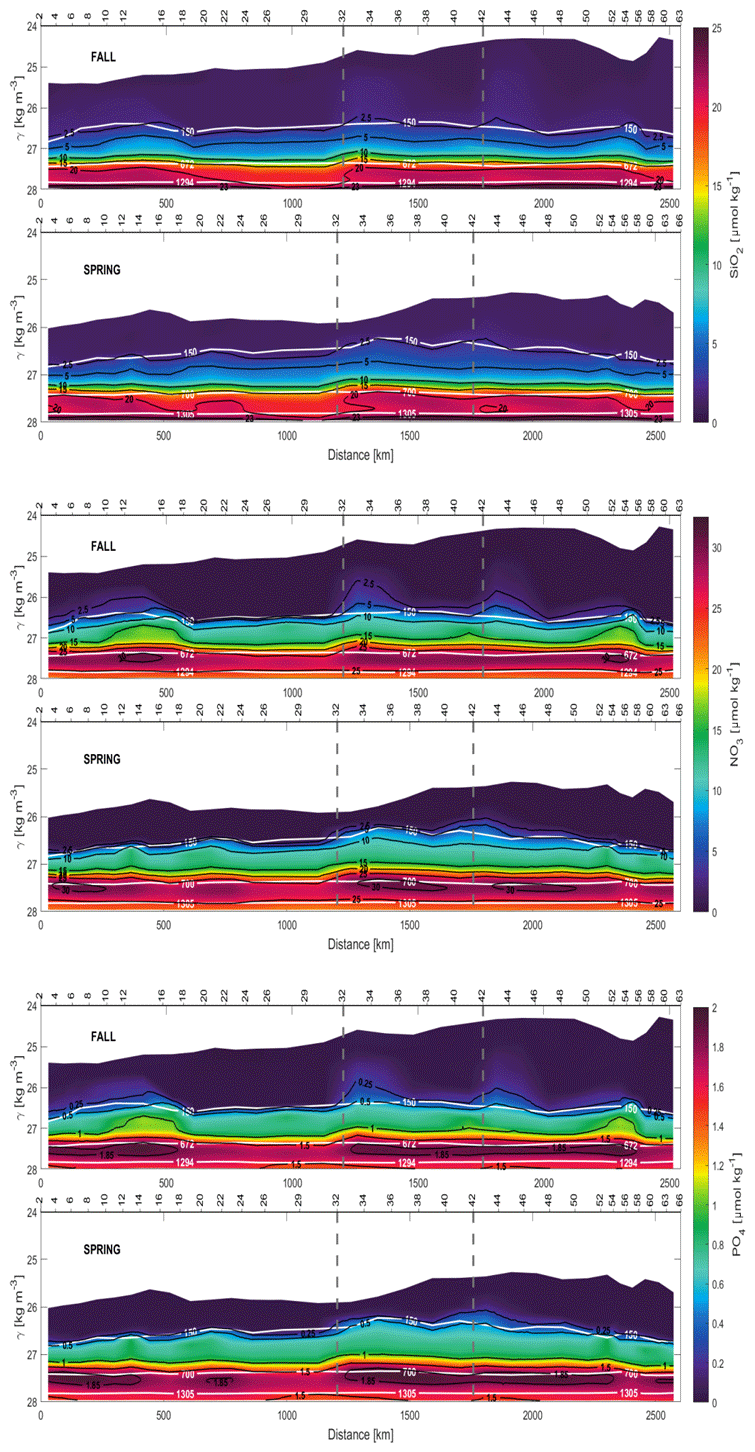
DOC concentrations are higher and more widely distributed in the water column in fall than in spring, when the DOC maximum values are more confined to surface and central waters (Figs. 8 and 6, Table 2). This fact is especially significant in the southern transect occupied by SACW (Fig. 6). SACW presents maximum concentrations of DOC 35–40 µmol L−1 lower than those found for NACW (Table 2). This difference is more pronounced in spring (Table 2). In addition, the fall DOC observations present a larger variability in central waters, as previously seen for INs. Lower DOC concentrations are observed for stations sampled in the western transect, while the highest concentrations are recorded in the stations next to the African slope with values above 100 µmol L−1 (Fig. 8). On the other hand, the high concentrations of DOC recorded at intermediate waters in the northern transect during both cruises are noteworthy (Figs. 8 and 6).

An inverse box model is applied to the hydrographic data from the two COCA cruises to provide the absolute velocity field across the three sections (Wunsch, 1978). This method has been widely applied in different areas of the Atlantic Ocean as an efficient method to obtain absolute geostrophic flows (Martel and Wunsch, 1993; Paillet and Mercier, 1997; Ganachaud, 2003a; Machín et al., 2006; Pérez-Hernández et al., 2013; Hernández-Guerra et al., 2017; Fu et al., 2018). Assuming geostrophy and the conservation of mass and other properties in the ocean bounded by the African coast and the hydrological sections, the velocity fields are obtained, allowing for an adjustment of freshwater flux and Ekman transports.
4.1 Selection of layers
The closed ocean where the inverse model is applied is divided into nine layers by means of the neutral densities defined by Macdonald (1998) and modified by Ganachaud (2003a) for the North Atlantic Ocean. This distribution is then slightly modified to include two layers instead of one between 26.85 and 27.162 kg m−3 by adding the isoneutral 27.035 kg m−3, as other authors have done previously at this side of the NASG (Comas-Rodríguez et al., 2011; Pérez-Hernández et al., 2013). The locations of the isoneutrals are represented in Fig. 2. The upper five layers group the surface and central waters, and the first layer until the isoneutral 26.44 kg m−3 is related to surface waters, while the four remaining layers between 26.44 and 27.38 kg m−3 are central waters. The intermediate waters are found in the next two layers between 27.38 and 27.82 kg m−3, while the deepest two layers below 27.82 kg m−3 contain the upper deep waters.
4.2 The system of equations
The inverse box model takes into account mass conservation per layer and also in the whole water column. The salinity is actually introduced as a salinity anomaly, which is also conservative within individual layers and in the whole water column (Ganachaud, 2003b). On the other hand, heat is introduced as a heat anomaly in the two deepest layers wherein it is also considered conservative. The salinity and heat are added as anomalies to improve the conditioning of the inverse model and get a higher rank in the system of equations by reducing the linear dependency between equations (Ganachaud, 2003b).
Therefore, the model is composed of a set of 22 equations (10 for mass conservation, 10 for salt anomaly conservation and 2 for heat anomaly conservation). Those equations are solved for 32 and 34 unknowns, comprised of 28–30 reference-level velocities in fall–spring, 3 unknowns for the Ekman transport adjustments (one unknown per section) and 1 unknown for the freshwater flux. The resulting system is undetermined and a Gauss–Markov estimator is used to select a solution by adding a priori information. This a priori information consists of the uncertainties for both the unknowns (Rxx) and the noise of the equations (Rnn).
4.2.1 Uncertainties of unknowns (Rxx)
The geostrophic velocity field is calculated in the central position between two consecutive stations. The isoneutral selected as the reference level is the deepest common γn for all the stations, 27.962 kg m−3 (Fig. 2). Initially, the reference level is considered a motionless level at which the geostrophic velocity is taken as null before applying the inversion. The variance of the velocity in the reference level at each location is used as a measure of the a priori information. These variances are calculated with an annual mean velocity extracted from the daily velocity provided by GLORYS. These velocities are interpolated to the reference-level depth. This reference-level depth is estimated from the climatological mean depth of 27.962 kg m−3 extracted from WOA13. The stations closer to the coast in the northern and southern transects have the highest variability in the velocity field. Machín et al. (2006) provide a comprehensive sensitivity analysis of the solution with respect to the a priori information in a domain just north of the one documented here. They conclude that the final mass imbalance is quite independent of both the reference level considered and the a priori uncertainties in the reference-level velocities.
The initial Ekman transports are estimated from the wind stress for both cruises. The uncertainty associated with these Ekman transports is related to the error in their measurements and the variability of the wind stress. A 50 % uncertainty is assigned to the initial estimate of Ekman transports. The initial freshwater flux is a climatological mean of 0.0171 Sv, which is also assigned an uncertainty of 50 % as reported in similar approaches (Ganachaud, 1999; Hernández-Guerra et al., 2005; Machín et al., 2006).
Both the Ekman transports and freshwater flux with their uncertainties are added to the model in the conservation equations corresponding to the shallowest layer of the mass transport and salt anomaly, as well as to the conservation equations of total mass transport and total salt anomaly.
4.2.2 Uncertainties in the noise of equations (Rnn)
The noise of each equation depends on the density field, the layer thickness and the uncertainties of the unknowns (Ganachaud, 1999, 2003b; Machín et al., 2006). In fact, Ganachaud (2003b) established that the largest source of uncertainty in conservation equations arises from the deviation of the baroclinic mass transport from the mean value at the time of the cruise. Thus, an analysis of the annual variability in the velocity field for the nine layers is performed. The velocity variability is examined in the mean depth between two successive isoneutral surfaces whose climatological mean depths are defined by WOA13. This variability is included in the inverse model as the a priori uncertainty or the noise of equations in terms of the variances of mass, salt anomaly and heat anomaly transports. The velocity variance from the annual mean velocity for each layer is estimated with GLORYS and transformed into transport values by multiplying the density and the vertical area of the section involved. These a priori transport uncertainties are presented in Table 3. Furthermore, the uncertainty assigned to the conservation equation in the total mass is the sum of the uncertainties from the rest of the nine conservative mass equations.
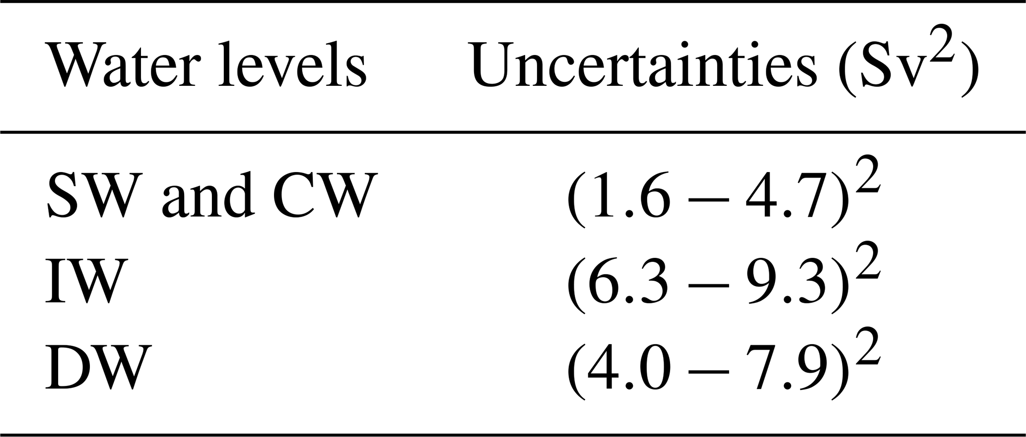
Table 3A priori noise of equations corresponding to the SW, CW, IW and DW levels at which the different water masses are transported.
The equations for salt and heat anomaly conservation depend on both the uncertainty of the mass transport and the variance of these properties (Ganachaud, 1999). In these cases, the a priori noise of each equation will not depend strictly on the water mass but on the layer considered, as shown in the following equation (Ganachaud, 1999; Machín, 2003):
where Rnn(Cq) is the uncertainty in the anomaly equation of the property (salt or heat anomaly); var(Cq) is the variance of this property; a is a weighting factor of 4 in the heat anomaly, 1000 in the salt anomaly and 106 in the total salt anomaly; and q is a given equation corresponding to a given layer.
As documented north of the Canary Islands, dianeutral velocities are of the order of 10−8 m s−1, while dianeutral diffusion coefficients are of the order of 10−6 m2 s−1 (Machín et al., 2006). The model results are much less affected by these values than by the reference velocities: a mean dianeutral velocity of 108 m s−1 would contribute only 0.01 Sv, a value much less than the lateral transports obtained from the inverse model. On the other hand, the inverse model provides information only from the box boundaries and cannot be used to infer any detailed spatial distribution of dianeutral fluxes within the box. Hence, mass transports between the layers due to dianeutral transfers are considered to be negligible compared to other sources of lateral transports and are not included in the inversion.
5.1 Velocity fields and mass transports
Figure 9 shows the reference-level velocities obtained after the inversion. The variance of these velocities is also estimated by the model. The uncertainties are much higher than the values themselves at around cm s−1. During fall all nonzero values are positive, while in spring they are negative. This difference is important mainly in the western and southern transects where the module of the velocity increases, reaching values of 0.3 and −0.16 cm s−1 in fall and spring, respectively. Furthermore, the estimated reference-level velocity values in the northern transect in spring are too small, 𝒪(10−4–10−5), while they take positive and significant values between 0.13 and 0.25 cm s−1 in some locations of this transect in fall.
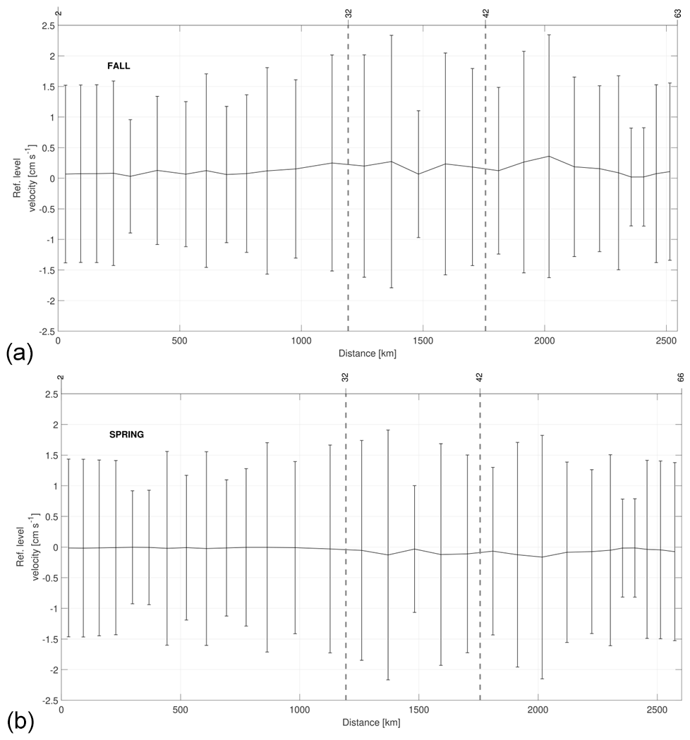
Figure 9Reference-level velocity at 27.962 kg m−3 and its standard deviation estimated by the inverse model during fall (a) and spring (b). The direction chosen for the representation is the same as in Fig. 2. The signs of the velocity are according to the geographical criterion; i.e., the velocities are positive–negative toward north–south in the northern and southern transects, and they are positive–negative toward east–west in the western transect.
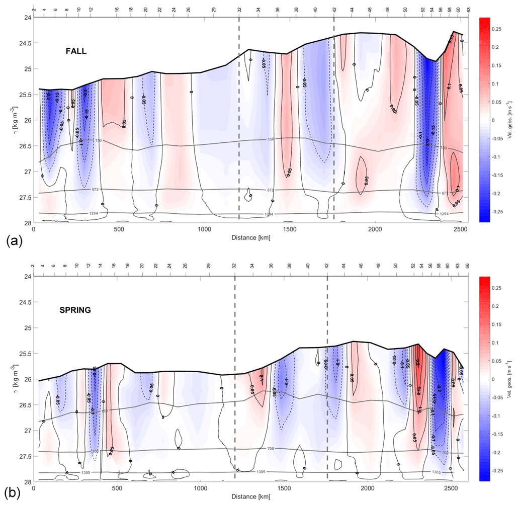
Figure 10Sections of the absolute geostrophic velocity with respect to γn during fall (a) and spring (b). The horizontal axis has the same direction as Fig. 2, and the criterion of the velocity signs is as in Fig. 9. The depths 150, 672–700 and 1294–1305 m are highlighted by grey isolines as in the γn sections in Figs. 4 and 5.
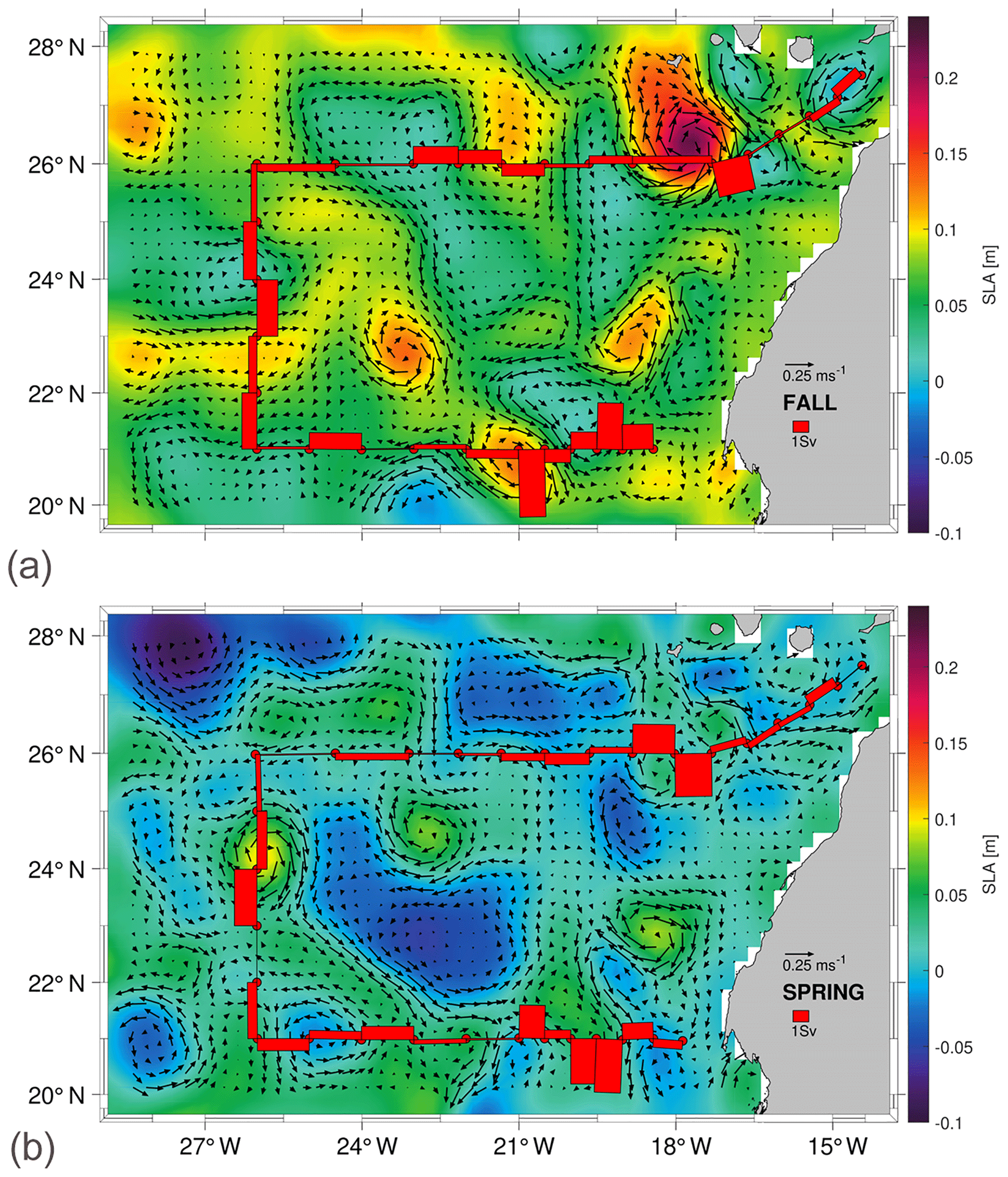
Figure 11Average derived geostrophic velocity and SLA during fall (a) in the course of the fist cruise and spring (b) in the course of the second cruise, extracted from AVISO+. The red bars represent the mass transports in the shallowest layer as estimated by the inverse model.
Once the geostrophic velocities at the reference level are estimated, they are integrated into the entire water column to obtain the absolute geostrophic velocities (Fig. 10). These results are validated by comparison with the surface geostrophic velocity and the sea level anomaly, SLA, derived from altimetry during the time period that each cruise was performed (Fig. 11). To do this, the average fields of SLA and geostrophic velocity at the sea surface are calculated during each cruise and shown as a synoptic result during both surveys. Furthermore, the mass transports at the shallowest layer (red bars in Fig. 11) are superimposed with the aim of comparing these transports with the average velocity field from altimetry. Remarkable mesoscale activity can be identified in both the absolute geostrophic velocity sections (Fig. 10) and the temporal average of SLA and the geostrophic velocity (Fig. 11). In this last case, the position of the structures at the SLA field is somewhat displaced with respect to their positions in the in situ velocity sections. For instance, an anticyclonic eddy is located between stations 10 and 16 in the N transect in both seasons. This eddy, observed in autumn with high velocities at intermediate layers, weakens in spring. This mesoscale structure could be part of the CEC (Sangrà et al., 2009). Furthermore, it coincides with the position of an anticyclonic eddy previously documented (Barceló-Llull et al., 2017a, b; Estrada-Allis et al., 2019).
In fall, two eddies are linked in the S transect, an anticyclonic one between stations 48 and 52 and a cyclonic one between stations 52 and 60, both associated with the CVFZ. In spring, two anticyclonic eddies are observed, one centered at station 36 and the other one at station 56, also associated with the CVFZ. In both seasons, mesoscale structures present a large vertical extension (Fig. 10). In fall, these structures have higher velocities at IW and DW levels and they also affect a higher extension along each transect. The SLA also shows a high-variability region with more intense structures in fall than in spring (Fig. 11).
Mesoscale structures are also visible in the vertical sections of NO3 and PO4 in fall, when their concentrations are higher than those observed in spring at similar locations (Fig. 7). Furthermore, high concentrations of DOC in fall at CW levels are recorded in the same area where the deep anticyclonic eddy is located, between stations 8 and 18 (Fig. 8). In spring, mesoscale structures in the vertical sections of INs and DOC at CW levels are less intense than in fall (Fig. 10). Nonetheless, DOC concentrations below the two anticyclonic structures at CW levels in spring are higher than in their surroundings.
The accumulated geostrophic mass transport is integrated to group the variability at different levels, with the first shallowest layer for SW, the next four layers for CW, then two layers for IW and the deepest two layers for DW (Fig. 12). The total accumulated geostrophic mass transport, integrated for all the nine layers, is also represented. The horizontal axis has the same direction as the rest of the vertical sections, and the three transects are separated by two vertical dashed grey lines. The Sverdrup (Sv) is used here as equivalent to 109 kg s−1. The positive–negative transport values indicate outward–inward transports from–to the box. The accumulated mass transports show a significant horizontal spatial variability, especially marked in the southern transect in accordance with the geostrophic velocity distribution (Fig. 10). The presence of significant mesoscale structures might be one of the sources of the total imbalances in the accumulated mass transport. In fall, the total imbalance is −1.43 Sv, and in spring it is 3.55 Sv (Table 4).
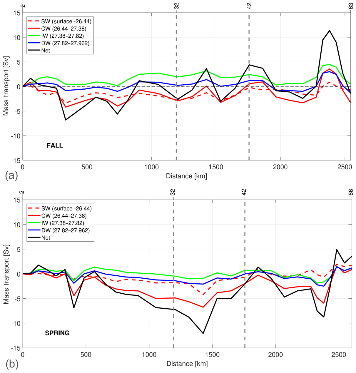
Figure 12Accumulated mass transport along the fall (a) and spring (b) cruises at the surface waters (SW, in red and dashed line), central waters (CW, in red line), intermediate waters (IW, in green line) and deep waters (DW, in blue line). The accumulated mass transport integrated for all nine layers is also represented. The horizontal axis has the same direction as Fig. 2. Negative–positive values of transports along the three transects indicate inward–outward transports in the box delimited by the three transects and the African coast.
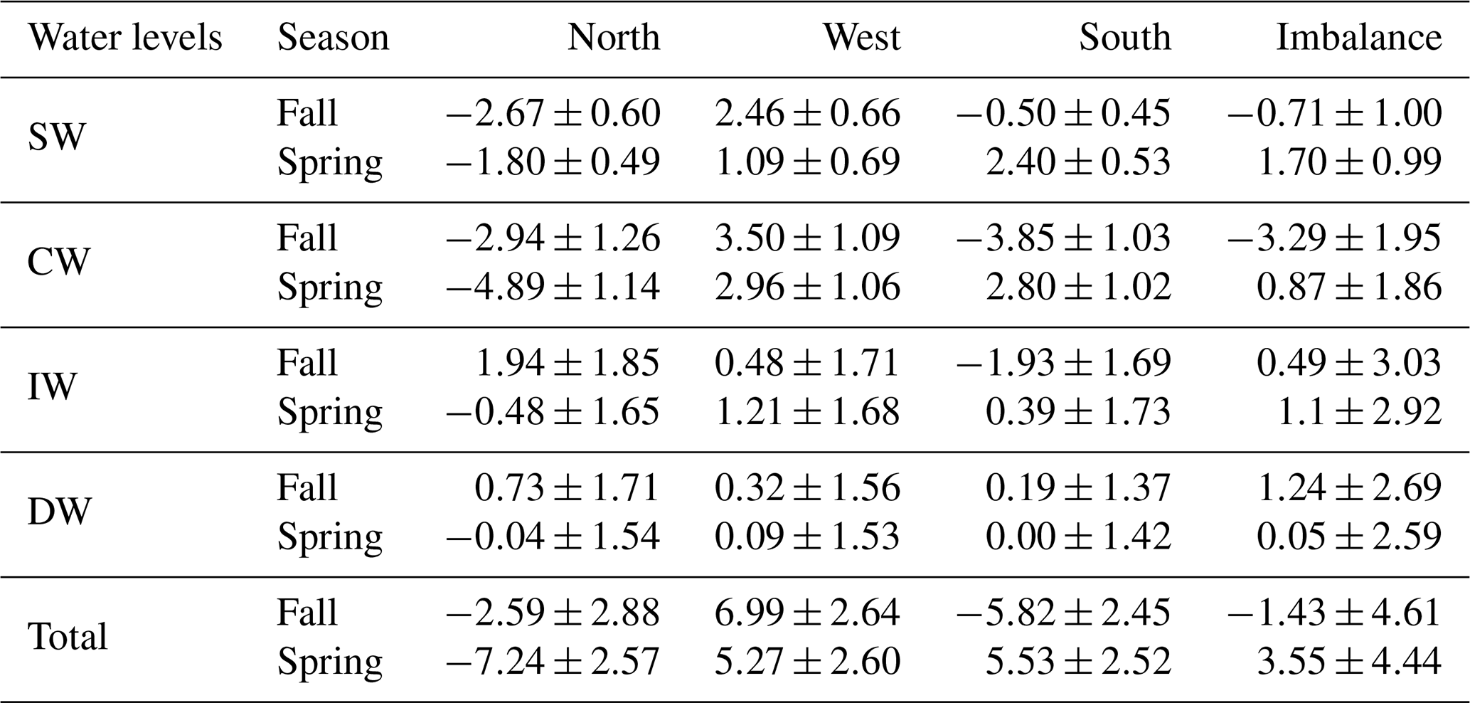
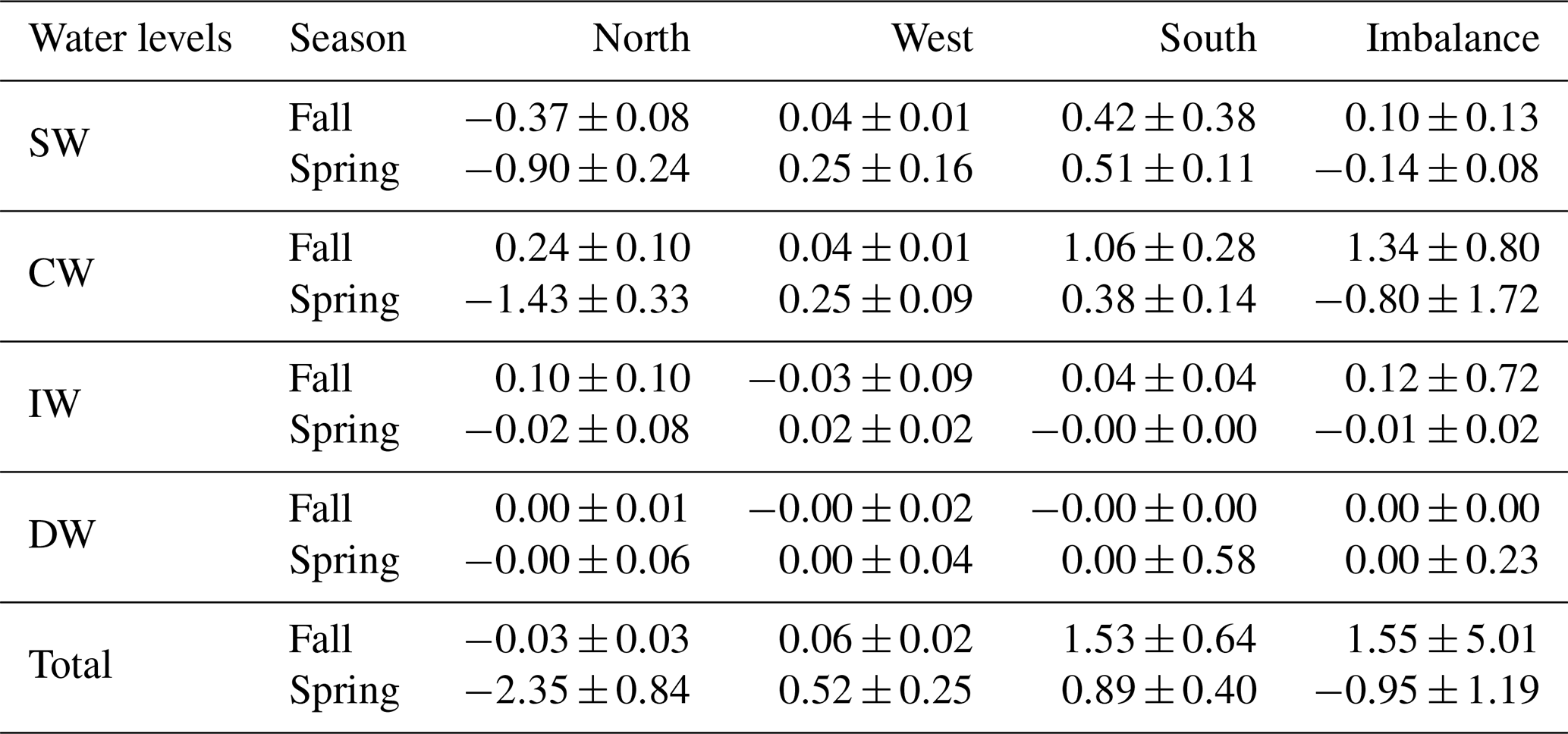
Table 4Mass transports with their errors (Sv) for SW, CW, IW and DW across the north, west and south transects for both seasons. Positive–negative values indicate outward–inward transports. The last row is the integrated transport for the entire water column in each transect, while the fourth column summarizes the imbalances in mass transport for both seasons.
On the other hand, the geostrophic mass transport can be integrated per layer and transect together with the total imbalance inside the box and the total mass transport uncertainty per layer (the black line and horizontal black bars in Fig. 13). Table 4 compiles these transports integrated for the different water levels, which are also represented geographically in Fig. 14. More than 65 % of the mass transport is given at SW and CW levels (Table 4). In fall, these water masses mostly move into the box across the northern and southern transects, with transports of and Sv, respectively; the mass leaves the box by flowing westward with a value of 5.96±1.75 Sv. In spring, water masses also move into the box mostly through the northern transect with Sv, but they leave along the western and southern transects with transports of 4.05±1.75 and 5.20±1.55 Sv, respectively. It is remarkable how the inward transport in fall across the southern transect is reversed to a net outward flow in spring at the southern transect (Fig. 13).

Figure 13Accumulated mass transports per transect at the north (N, magenta line), west (W, dark grey line) and south (S, blue line) transects during fall (a) and spring (b). See Table 2 for the γn values bounding every water layer. Negative–positive values indicate inward–outward transports as in Fig. 12. Mass conservation in the whole domain is shown by the black line. The horizontal bars represent the uncertainties estimated by the model.
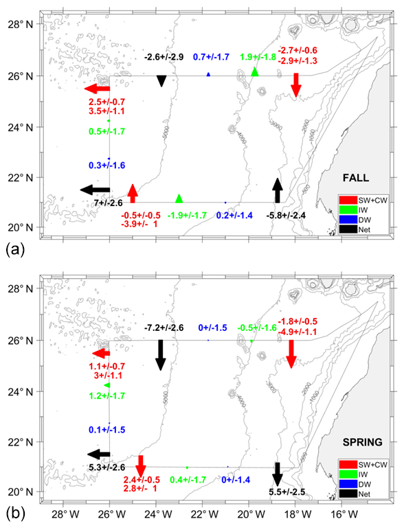
Figure 14Mass transports with their errors (Sv) at the surface and central waters (SW+CW, red arrow), intermediate waters (IW, green arrow), and deep waters (DW, blue arrow) across every transect during fall (s) and spring (b). Negative–positive values indicate inward–outward transports as in Fig. 12. The arrows in each transect are located at positions that optimize their visibility, representing the integrated transports along each transect. The values of transports at SW (dark red) are given next to the integrated values of transports at CW levels (in red).
The position of the CVFZ in both seasons could partly explain the seasonal variability in the mass transports at central levels (Fig. 15). In fall, the CVFZ is located further from the African coast, so SACW is present at almost all stations of the south transect. This location of the CVFZ prevents a latitudinal mass transport from north to south. However, in spring the CVFZ is closer to the African slope, allowing for an important mass transport from north to south.

Figure 15Mean salinity and mean geostrophic velocity at 156 m extracted from GLORYS during fall (b) and spring (b). The black line indicates the position of isohaline 36 at this depth, used to identify the CVFZ. The red bars represent mass transports in the shallowest layer as estimated by the inverse model.
Between 5 % and 30 % of the mass transport is given in intermediate levels (Table 4). In fall, the intermediate water transport is directed northward in the southern transect with Sv, and it leaves the box with 1.94±1.85 and 0.48±1.71 Sv across the northern and western transects, respectively. During spring, this transport weakens and changes its direction in the northern and southern transects with transports of and 0.39±1.73 Sv, respectively, increasing its westward transport to 1.21±1.68 Sv.
The mass transport in deepwater layers barely exceeds 3 % (Table 4). An exception is the 8 % given in the northern transect during fall when the estimated transport is 0.73±1.71 Sv. During both cruises the transport at deep levels was nearly balanced.
5.2 Nutrient and DOC transports
DOC and IN transports are obtained by multiplying their concentration by mass transports. DOC, INs and geostrophic velocities are obtained at different locations, so they need to be interpolated to a common grid. In the case of DOC, the velocities are horizontally interpolated to the locations where the concentrations of DOC are taken, and, in a second step, the concentrations of DOC are linearly interpolated to the depths of the geostrophic velocities. On the other hand, the in situ measurements of INs are scarce at IW and DW where their concentrations become higher. Therefore, instead of using the observational data, the average outputs of GLORYS-BIO are used to estimate the IN transports. SiO2, NO3 and PO4 mean concentrations are interpolated to the grid nodes for which the geostrophic velocities are estimated by the inverse model.
DOC transports are obtained by subtracting a refractory concentration of 40 µmol L−1 from the measured DOC (e.g., Santana-Falcón et al., 2017). This is done because the refractory fraction renewal is thousands of years, a period much longer than the time required in the processes we are focused on (Hansell, 2002). On the other hand, it should be emphasized that DOC transports may be underestimated due to the scarcity of available measurements.
The IN transport values are presented in the text always ordered as SiO2, NO3 and PO4 (Figs. 16 and 17). Tables 5, 6 and 7 summarize those transports integrated per water level and transect. The errors are relative to the mass transport errors and are calculated as the standard deviations of IN transports. The DOC transport estimates per layer and transect are also shown in Fig. 17 and summarized per water level and transect with their relative error (calculated as in the IN transports) in Table 8. In order to be able to compare our transport values of INs and DOC with those reported by other authors, equivalent units are employed for IN (kmol s−1) and DOC transports (×108 mol C d−1).
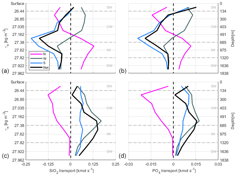
Figure 16Accumulated SiO2 and PO4 transports (kmol s−1) at transects in the north (N, magenta line), west (W, dark grey line) and south (S, blue line) during fall (a, b) and spring (c, d). See Table 2 for the γn values bounding every water layer. Negative–positive values indicate inward–outward transports as in Fig. 12. The net transport in the whole box is shown by the black line.
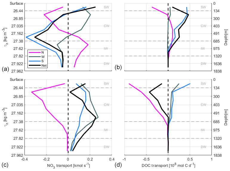
Figure 17Accumulated NO3 transports (kmol s−1) and accumulated DOC transports (108 mol C d−1) at transects in the north (N, magenta line), west (W, dark grey line) and south (S, blue line) during fall (a, b) and spring (c, d). See Table 2 for the γn values bounding every water layer. Negative–positive values indicate inward–outward transports as in Fig. 12. The net transport in the whole box is shown by the black line.
Table 5SiO2 transports and their errors (kmol s−1) for CW, IW and DW for the north, west and south transects. Positive–negative values indicate outward–inward transports. The last row is the integrated transport in the entire water column in each transect, and the last column represents the net transport for this variable inside the box.
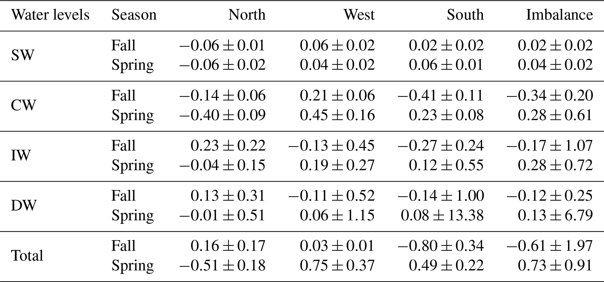
Table 6NO3 transports and their errors (kmol s−1) for CW, IW and DW for the north, west and south transects. Positive–negative values indicate outward–inward transports. The last row is the integrated transport in the entire water column in each transect, and the last column represents the net transport of this variable inside the box.
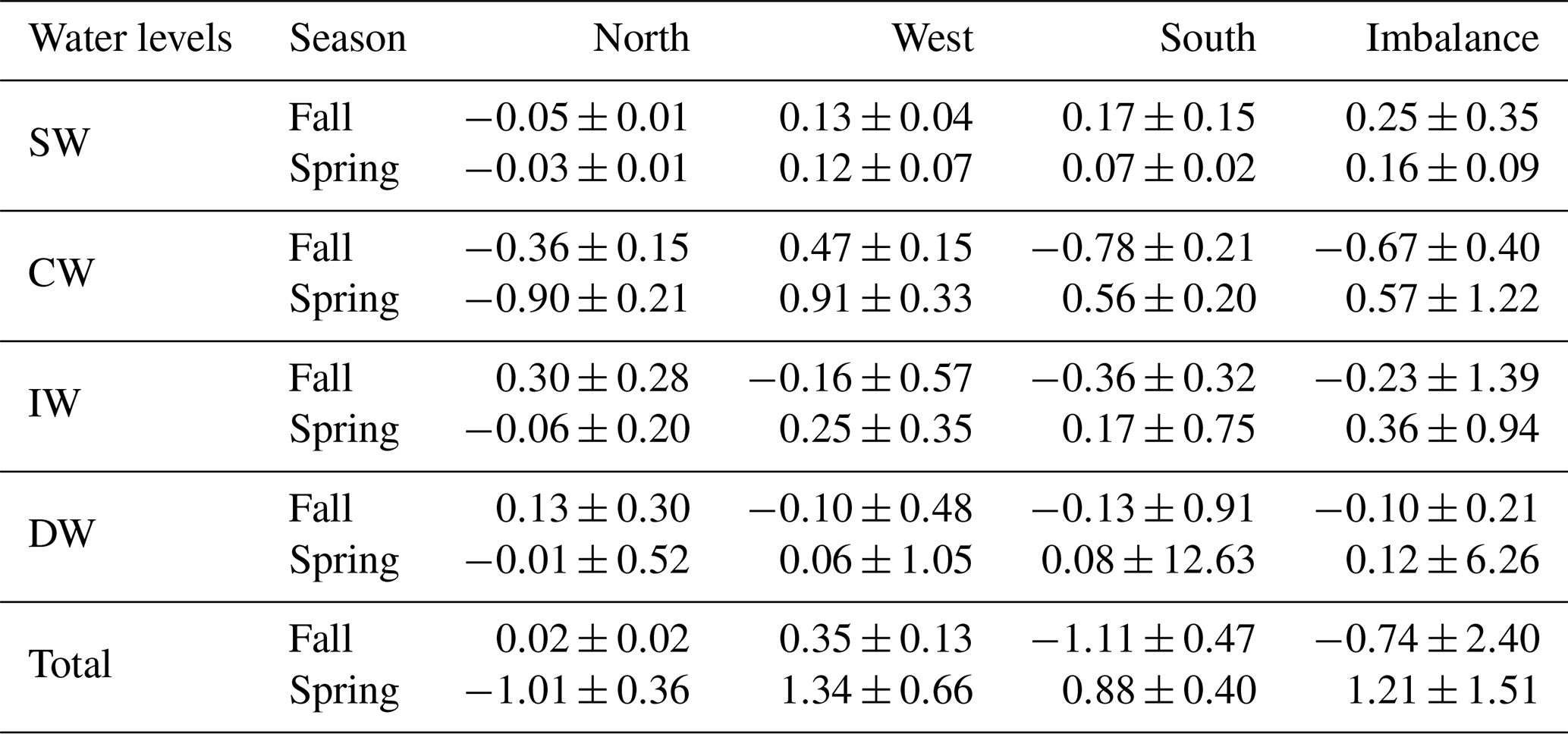
Table 7PO4 transports and their errors (kmol s−1) for CW, IW and DW for the north, west and south transects. Positive–negative values indicate outward–inward transports. The last row is the integrated transport in the entire water column in each transect, and the last column represents the net transport of this variable inside the box.
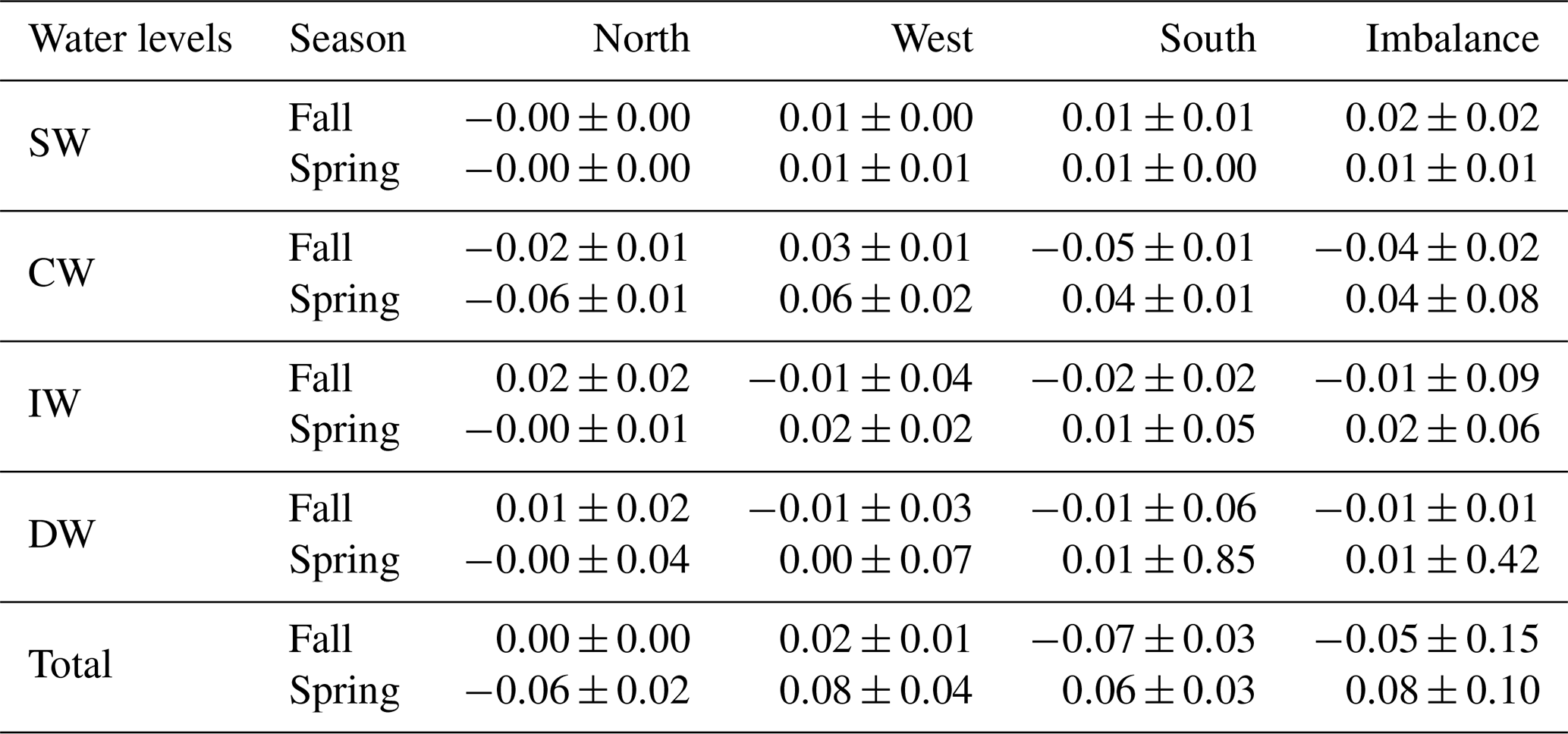
INs enter the domain both from the north and south at CW in fall. At the northern transect the transports are relatively low, while at the southern one transports double the amount coming from north, with , and kmol s−1. In spring, instead, the IN transports change their direction in the southern transect and only enter from the north, with values double those during fall, , , kmol s−1. On the other hand, IN transports at CW layers are overall westward with low values in fall, while in spring IN transports are southward and westward.
At IW levels, during fall the IN transports are inward through the southern transect, with , and kmol s−1, and to a lesser extent through the western transect. Outward transports are observed through the northern transect with 0.23±0.22, 0.30±0.28 and 0.02±0.02 kmol s−1. In spring, the INs enter weakly through the northern transect and leave the box, crossing the western and southern transects with significant values of 0.19±0.27 and 0.12±0.55 kmol s−1 for SiO2, 0.25±0.35 and 0.17±0.75 kmol s−1 for NO3, and 0.02±0.02 and 0.01±0.05 kmol s−1 for PO4. In summary, while in fall the main IN transports are in the south to north direction, in spring they are mainly southwestward like the mass transport behavior at these levels during this season (Table 4).
Finally, at DW during both seasons, the net transports of the three nutrients are similar to those at IW but with smaller values due to the low velocities at these depths, despite their high nutrient concentrations (Figs. 16 and 17). Furthermore, the relative error in these layers is always larger than the IN transport values.
In spring, DOC transports at SW and CW levels are the same order of magnitude and 1 order of magnitude higher than those at IW levels. In turn, these transports at IW levels are 1 order of magnitude higher than those at DW levels during this season. In contrast, during fall at the northern transect DOC transports have the same magnitude in SW, CW and IW, and they are 1 order of magnitude smaller than those at CW levels during spring (Table 8). In this season, DOC transports at SW and CW in the western transect have unrealistically small values likely related to the low number of measurements made in this transect during fall. DOC transports through the northern transect could also be somewhat underestimated for the same reason. However, at the southern transect during fall, the result is of the same order of magnitude as in spring.
In spring, DOC transports behave in a similar way in the entire water column. At SW and CW levels, mol C d−1 enters through the northern transect, mol C d−1 of which leaves the box through the southern transect, approximately half of it through the western transect. During fall, there is an important outward DOC transport at SW, CW and IW levels, especially southward through the southern transect at SW and CW levels, with a total of mol C d−1 (Table 8).
Table 8DOC transports and their errors (108 mol C d−1) for CW, IW and DW for the north, west and south transects. Positive–negative values indicate outward–inward transports. The last row is the integrated transport in the entire water column in each transect, and the last column represents the net transport for this variable inside the box. These values are transports of non-refractory DOC, which is obtained by subtracting an amount of 40 µmol L−1 from the measured DOC.
Two opposite trends can be observed when both cruises are compared. In fall the IN net transports are , and kmol s−1 at CW levels; , and kmol s−1 at IW levels; and , and kmol s−1 at DW levels. The amount of nutrients entering the box is larger than those leaving the box, with the exception of the shallowest level at which the INs leave the box (Tables 5, 6 and 7 and Figs. 16 and 17). On the other hand, the net DOC transports are outward for SW, CW and IW levels with mol C d−1 at SW levels, mol C d−1 at CW levels and mol C d−1 at IW (Table 8 and Fig. 17).
In contrast, during spring a net outward transport is obtained for the three INs with 0.28±0.61, 0.57±1.22 and 0.04±0.08 kmol s−1 at CW, 0.28±0.72, 0.36±0.94 and 0.02±0.06 kmol s−1 at IW, and 0.13±6.79, 0.12±6.26 and 0.01±0.42 kmol s−1 at DW (Tables 5, 6 and 7, and Figs. 16 and 17). The DOC net transports are inward with mol C d−1 at SW level; mol C d−1 at CW levels; and mol C d−1 at IW levels (Table 8 and Fig. 17).
The circulation patterns in the studied area of the Canary Basin change significantly, showing a temporal variability from fall to spring. The differences between the two seasons are reflected in the estimated mass transports for both cruises (Figs. 13 and 14 and Table 4).
Trade winds are intense all year long between the Canary Islands and Cape Blanc (26 to 21∘ N), and they generate a quasi-permanent upwelling in this region north of Cape Blanc. In contrast, the developed EBUS intensity and its offshore development change from fall to spring (Benazzouz et al., 2014). At the beginning of spring there is a strong heating that generates a sharp water stratification, particularly in the interior ocean of the NASG, and a very intense upwelling that makes the EBUS strongly develop far offshore. In early fall, the EBUS weakens and becomes a shallower front that approaches towards the coast (Pelegrí and Benazzouz, 2015a). In fact, the variability related to its location and intensity may be the reason that the estimated mass transports in the north–south direction are distributed between levels of central waters and intermediate waters in fall and that in spring these mass transports parallel to the coast are confined to the shallowest layers at central waters. On the other hand, these changes in the EBUS and the water stratification may also be related to the westward mass transports, which in fall are accentuated and confined to the levels of SW and CW as a shallow Ekman transport, while in spring the lateral westward transport is distributed from the sea surface down to IW levels (Table 4 and Fig. 13).
SW transports through the N and W transects show similar patterns, but in fall they are significantly more intense than in spring. In addition, CW level transports through these two transects also show similar patterns, with low variability between the two seasons. The largest differences are observed in the estimated transports through the S transect, which change from fall to spring; the transport is northward during fall and southward during spring. This observed variability in the transports in SW and CW levels in the southern part of the domain is likely related to the seasonal changes in the position of the CVFZ, which is in turn related to the seasonal changes in the North Atlantic tropical gyre (NATG) south of the domain (Pelegrí et al., 2017). The fact that the Intertropical Convergence Zone moves southward in winter and northward in summer affects the circulation patterns south and north of Cape Blanc (Lázaro et al., 2005; Stramma et al., 2008; Peña-Izquierdo et al., 2012). While in fall the CVFZ crosses the S transect in its westernmost position, in spring it moves closer to the African coast. The output of the GLORYS model matches the observations during both seasons (Fig. 15). In addition, the dynamics described by the geostrophic field of GLORYS also agree with the velocity field and the mass transports at CW levels estimated by the inverse model in the S transect for both seasons.
GLORYS velocity outputs also reproduce mesoscale and submesoscale features associated with the CVFZ (Pérez-Rodríguez et al., 2001; Martínez-Marrero et al., 2008), which are observed directly in the S transect of the velocity sections (Fig. 10) and in the accumulative mass transport (black line in Fig. 13). Specifically during fall, the reported eddies significantly boost transport at the SW and CW levels from south to north. All these results at CW levels are consistent with the late summer and fall growth of the Mauritania Current and of the PUC, as well as with the decrease in the NATG currents and the weakening of the Guinea Dome in winter and spring (Siedler et al., 1992; Lázaro et al., 2005; Peña-Izquierdo et al., 2012; Pelegrí and Peña-Izquierdo, 2015; Pelegrí and Benazzouz, 2015a). The estimated transports at IW also show seasonal changes between fall and spring. This region is featured by a late summer northward progression of AAIW observed in fall and by a weak southward flow of MW in spring (Machín et al., 2010). The northward significant mass transports observed in fall at the north and south transects is consistent with the northward spreading documented for AAIW (Machín and Pelegrí, 2009; Machín et al., 2010).
In general, the estimated transport of the three INs shows similar patterns, marked by the mass transport variability during both seasons. The level with the highest transport for all the nutrients in both seasons is the deepest CW layer. This is quite in agreement with the local maximum of remineralization found for all tracers in the upper intermediate layer by Fernández-Castro et al. (2018).
CW levels are featured by a relatively high biological production and therefore a nutrient deficit, as well as by large geostrophic velocities. During fall the amount of INs that enters the box through the N and S transects is larger than the IN quantity that leaves the box through the W transect. In spring, on the other hand, the amount of INs transported outward through the W and S transects is larger than the INs that enter from the north.
At IW levels the concentrations of INs are high and stable, related to the dominant remineralization process. During spring, the spatial distribution of the three IN transports are the same as at CW levels, with smaller values. In this season the transports of INs are directed westward through the W transect towards the oligotrophic open ocean. In fall, the IN transports at IW levels have a behavior different than at CW levels, which is the main transport in the south–north direction.
The most significant differences between the DOC transports in fall and spring are obtained in the first and second shallowest layers in which there are high lateral velocities and the euphotic layer. During fall, the DOC quantity that enters by the north transect is a third of the amount that leaves the region by the south. In the spring, however, the large amount of DOC that enters the domain from the north is double the quantity that leaves it by the S transect, while a quarter leaves by the western transect.
In spring, when the stratification is less marked, the most significant and deepest transports of INs are observed toward the open ocean in central and intermediate water levels. However, in fall, when the water column is more stratified and the upwelling process is the main physical forcing for nutrient supply at CW levels (Pastor et al., 2013), the IN transports toward the oligotrophic interior ocean are less than in spring. In fact, while in the western transect during spring the IN transports increase with depth to their maximum values at the deepest central layer, in fall the opposite occurs, since the westward IN transports decrease with depth until canceling at the last central layer; these transports reverse towards the coast at the two intermediate layers (grey line in Figs. 16 and 17).
On the other hand, DOC transports are deeper and more intensified toward the open ocean during spring than in fall. Nonetheless, in fall there is an important and deeper transport of INs in a direction parallel to the coast. In fact, at IW DOC concentrations accumulate next to the African coast in the upwelling region. Furthermore, inside the upwelling region at the N and S transects in fall, the two observed mesoscale anticyclonic eddies could enhance this process.
The variability in the intensity of the stratification, the strength of upwelling, and the position of the boundary between the upwelling and the oligotrophic interior ocean, together with important mesoscale and submesoscale structures, control the nutrient availability at CW and IW waters. It is also deduced from DOC transport estimates that the upwelling drives the changes in the size of the high-production domain and, equivalently, the position of the eastern boundary of the oligotrophic region in this area (Pastor et al., 2013).
The estimated transports of INs and DOC tell us that in fall there is a pronounced import of INs into the domain (with the exception of the SW layer) and a moderate export of DOC, especially at CW and IW levels. On the other hand, during spring there is a pronounced export of INs from the domain at CW and IW levels and a slight import of DOC at the shallowest CW levels and at the SW layer.
The observations used so far provide nutrient fluxes during two cruises performed only in two seasons of the years 2002 and 2003. Thus, the full seasonal variability cannot be addressed with in situ observations from those years. Instead, in this section the seasonal variability is analyzed based on numerical modeling outputs to depict the context in which the in situ nutrient fluxes are evaluated. To do so, the time span that contains both cruises of the COCA project from 1 July 2002 to 30 June 2003 is analyzed with a climatological approach: summer comprises the months from July to September, fall from October to December, winter from January to March and finally spring from April to June.
The analyses are performed at three different key points located in each transect during both cruises (Fig. 18). The northern point is located between stations 18 and 20, the western one between stations 36 and 38, and the southern point between stations 50 and 52. These locations are chosen as the most representative points of each transect. Nutrient profiles at each transect are analyzed for both seasons, and the key points are selected for which the three nutrient profiles are consistent with their average distribution. In the case of the northern and southern transects, the key points are located at the intermediate point between the upwelling area and the oligotrophic open ocean, where the nutrient concentrations remain fairly stable among seasons. At the western transect, the middle position is considered to be the representative point since all nutrient profiles are markedly homogeneous along this transect, and, in addition, nutrient concentrations are rather constant from fall to spring (middle column in Fig. 6).
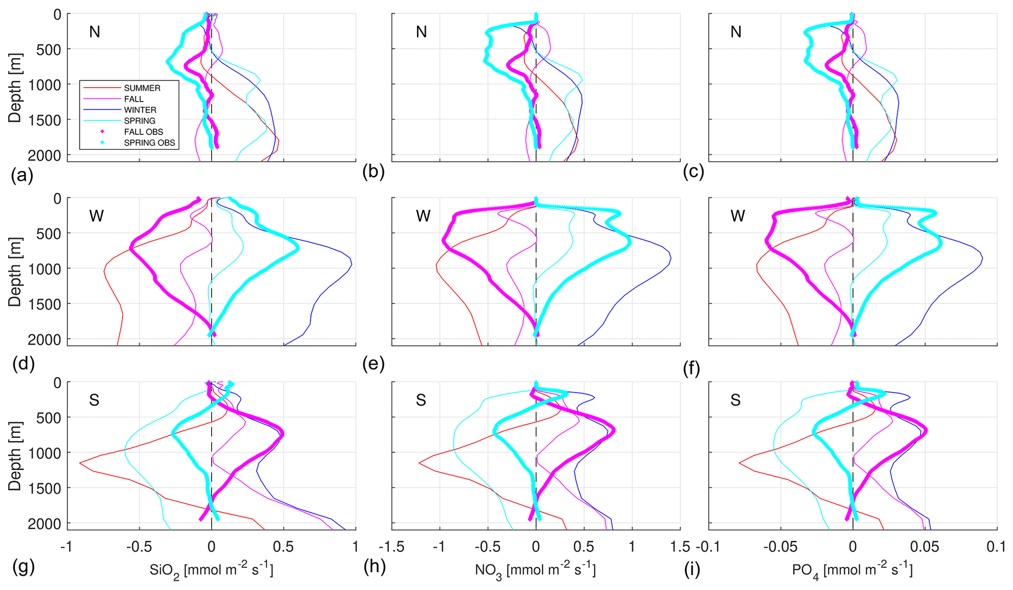
Figure 18Numerical modeling of seasonal SiO2 (a, d, g), NO3 (b, e, h) and PO4 (c, f, i) fluxes (mmol m−2 s−1) at the three key points (N: in the north transect, a, b, c; W: in the west transect, d, e, f; S: in the south transect, g, h, i). The following are represented: summer, from July to September, by the thin red line; fall, from October to December, by the thin magenta line; winter, from January to March, by the thin blue line; and spring, from April to June, by the thin cyan line. The three nutrient fluxes observed in situ in fall (magenta) and spring (cyan) are also plotted with thicker dotted lines.
The biogeochemical model is combined with the physical model to obtain the seasonal nutrient fluxes at the three key points (Fig. 18). Overall, nutrient fluxes are negligible at the surface, where nutrients are depleted as a result of photosynthetic activity. On the other hand, nutrient fluxes usually present their largest values in the depth range from 500 to 1000 m, as a combination of relatively large currents and nutrient concentrations. Nutrient fluxes at the northern point present a somewhat complex vertical structure, with opposite patterns above and below approximately 600 m of depth. Above 600 m of depth, nutrient fluxes are northward in fall, while they are southward in the rest of the seasons. Below that depth, nutrient fluxes are southward in fall, while they are northward for the remaining seasons. Once the nutrient fluxes from in situ observations are considered, some differences arise from both datasets. On the one hand, during spring both results indicate a southward nutrient flux above 500 m, while below that depth nutrient fluxes are southward for the in situ observations and northward for the numerical results. On the other hand, in fall the nutrient fluxes are southward in the entire water column for the in situ observations, while for the numerical results they are northward in the upper 500 m of depth and southward in the remaining water column. In any case, the intensities in the nutrient fluxes from in situ data and from numerical modeling outputs are quite similar.
At both the western and southern points, the fluxes present a much simpler vertical structure. At the western point, nutrient fluxes in the whole water column are westward in winter and spring, while they are eastward in summer and fall. Maximum nutrient fluxes are obtained for winter and summer seasons, while minimum values are estimated for the spring and fall seasons. Nutrient fluxes estimated from in situ observations present the same direction as those estimated by the numerical model in both seasons, though somehow the in situ results duplicate the numerical values. At the southern point, nutrient fluxes are southward in fall and winter, while they are mainly northward in spring and summer. The southward nutrient flux modeled in summer in the upper 500 m of depth might be noteworthy. Nutrient fluxes from the in situ observations largely coincide with the numerical results, particularly in their directions below 300 m of depth. In this case, the intensity from the numerical result is double that from the in situ observation in spring, while roughly the opposite occurs in fall.
An inverse box model has been applied in the eastern North Atlantic to estimate mass, nutrient and organic matter transports during spring and fall. The currents estimated are largely affected by mesoscale features related to the Canary Eddy Corridor and to the Cape Verde Frontal Zone. The net mass transport at SW+CW levels coincides in both seasons in the N transect with a southward flow of 5.61±1.86 Sv in fall that increases in spring to 6.69±1.63 Sv. In the W transect the net westward mass transport at the SW+CW levels weakens from a value of 5.96±1.75 Sv in fall to 4.05±1.75 Sv in spring. The most remarkable change in the net mass transport at SW+CW layers occurs in the southern transect where in fall the net mass transport is northward with a value of 4.35±1.48 Sv, while in spring it is southward with a value of 5.20±1.55 Sv.
At IW layers, the net transport in the south–north direction is intense and northward in fall at 1.94±1.85 Sv, while it weakens and reverses southward in spring to 0.48±1.65 Sv. In the W transect, the net westward mass transport at IW layers is less intense in fall at 0.48±1.71 Sv than in spring at 1.21±1.68 Sv. Finally, the net mass transport at DW levels is small compared to the other water levels, with the exception of the 0.73±1.71 Sv estimated in the N transect during fall.
This geographical distribution of the mass transports is consistent with a southwestward flow mainly fed by the Canary Current. On the other hand, the temporal variability of mass transports in the southern section is likely related to a zonal shift of the CVFZ, which might be located in its westernmost position in fall, bolstering the presence of waters from the South Atlantic in the domain considered. At intermediate levels the significant northward transport observed at both the north and south transects during fall must be highlighted.
With regard to the IN and DOC net transports, in fall the domain works as a nutrient sink, with a total IN net import of 0.61±1.97, 0.74±2.40 and 0.05±0.15 kmol s−1 for SiO2, NO3 and PO4, respectively, while in spring it works as a source of nutrients, with a total nutrient net export of 0.73±0.91, 1.21±1.51 and 0.08±0.1 kmol s−1. It is also observed that the net DOC outward transport is mol C d−1 in fall when the domain acts as a source of DOC, while the net inward value of mol C d−1 describes it as a DOC sink in spring.
With respect to the lateral transports of both INs and DOC to the open ocean through the W transect, during spring there is a continuous westward IN transport of 0.75±0.37, 1.34±0.66 and 0.08±0.04 kmol s−1 for SiO2, NO3 and PO4, respectively, in the entire water column. These transports coincide with an important westward transport of DOC of mol C d−1, mainly at SW and CW levels. In fall, these transports weaken at CW and reverse at IW, which means that the net westward transport of INs is smaller than in spring, with values of 0.03±0.01, 0.35±0.13 and 0.02±0.01 kmol s−1 for SiO2, NO3 and PO4. Westward transports of DOC during fall are lower than in spring, with only mol C d−1.
Overall, nutrient fluxes estimated with in situ observations compare well with those estimated from numerical modeling outputs. The main differences in their directions are obtained in the northern section, while the differences in the western and southern sections are mainly related to their intensity.
It is still necessary to continue building an understanding of physical and biogeochemical processes and the interactions between the productive EBUS and the interior ocean in its vicinity, especially in dynamically complex regions such as this area where the EBUS interacts with both the CVFZ and mesoscale features. Larger and more robust hydrological and biogeochemical databases would help to achieve this goal.
To access the COCA data, please contact the main researchers of the project: Javier Arístegui (javier.aristegui@ulpgc.es) and Carlos Manuel Duarte (carlos.duarte@kaust.edu.sa).
JA and CMD collected and analyzed the biogeochemical data from the two COCA oceanographic cruises. NB conceived the analysis of the physical variables and associated physical processes. NB carried out the transport calculations and developed the comparison of the in situ versus modeling results with the support of FM. NB prepared the paper with contributions from FM. All authors participated in the scientific interpretation and discussed the main results.
The authors declare that they have no conflict of interest.
This work has been done thanks to the project COCA (REN2000-U471-CO2-02-MAR), which is funded by the Spanish National Research Program and the European Regional Development Fund (MINECO/FEDER). Currently, Nadia Burgoa is working on her PhD, with a fellowship funded by the Spanish Ministry of Economy and Competitiveness.
This research has been supported by the Spanish National Research Program, the European Regional Development Fund (MINECO/FEDER) through project FLUXES (project no. CTM2015-69392-C3-3-R).
This paper was edited by Eric J.M. Delhez and reviewed by Aissa Benazzouz and one anonymous referee.
Alonso-González, I. J., Arístegui, J., Vilas, J. C., and Hernández-Guerra, A.: Lateral POC transport and consumption in surface and deep waters of the Canary Current region: A box model study, Global Biogeochem. Cy., 23, GB2007, https://doi.org/10.1029/2008GB003185, 2009. a
Álvarez, M. and Álvarez-Salgado, X. A.: Chemical tracer transport in the eastern boundary current system of the North Atlantic, Cienc. Mar., 35, 123–139, 2009. a
Álvarez-Salgado, X. A., Arístegui, J., Barton, E. D., and Hansell, D. A.: Contribution of upwelling filaments to offshore carbon export in the subtropical Northeast Atlantic Ocean, Limnol. Oceanogr., 52, 1287–1292, https://doi.org/10.4319/lo.2007.52.3.1287, 2007. a
Arístegui, J., Sangrá, P., Hernández-León, S., Cantón, M., Hernández-Guerra, A., and Kerling, J.: Island-induced eddies in the Canary Islands, Deep-Sea Res. Pt. I, 41, 1509–1525, 1994. a
Arístegui, J., Barton, E. D., Álvarez-Salgado, X. A., Santos, A. M. P., Figueiras, F. G., Kifani, S., Hernández-León, S., Mason, E., Machú, E., and Demarcq, H.: Sub-regional ecosystem variability in the Canary Current upwelling, Prog. Oceanogr., 83, 33–48, 2009. a
Azam, F.: Microbial control of oceanic carbon flux: the plot thickens, Science, 280, 694–696, 1998. a
Barceló-Llull, B., Sangrà, P., Pallàs-Sanz, E., Barton, E. D., Estrada-Allis, S. N., Martínez-Marrero, A., Aguiar-González, B., Grisolía, D., Gordo, C., Rodríguez-Santana, Á., Marrero-Díaz, Á., and Arístegui, J.: Anatomy of a subtropical intrathermocline eddy, Deep-Sea Res. Pt. I, 124, 126–139, 2017a. a, b
Barceló-Llull, B., Pallàs-Sanz, E., Sangrà, P., Martínez-Marrero, A., Estrada-Allis, S. N., and Arístegui, J.: Ageostrophic Secondary Circulation in a Subtropical Intrathermocline Eddy, J. Phys. Oceanogr., 47, 1107–1123, https://doi.org/10.1175/JPO-D-16-0235.1, 2017b. a
Barton, E. D.: The poleward undercurrent on the eastern boundary of the subtropical North Atlantic. Poleward flows along eastern ocean boundaries, Springer, New York, NY, 82–95, 1989. a
Barton, E. D., Arístegui, J., Tett, P., Canton, M., García-Braun, J., Hernández-León, S., Nykjaer, L., Almeida, C., Almunia, J., Ballesteros, S., Basterretxea, G., Escanez, J., García-Weill, L., Hernández-Guerra, A., López-Laatzen, F., Molina, R., Montero, M. F., Navarro-Peréz, E., Rodríguez, J. M., Van Lenning, K., Vélez, H., and Wild, K.: The transition zone of the Canary Current upwelling region, Prog. Oceanogr. 41, 455–504, https://doi.org/10.1016/S0079-6611(98)00023-8, 1998. a, b, c
Benazzouz, A., Pelegrí, J. L., Demarcq, H., Machín, F., Mason, E., Orbi, A., Peña-Izquierdo, J., and Soumia, M.: On the temporal memory of coastal upwelling off NW Africa, J. Geophys. Res.-Oceans, 119, 6356–6380, https://doi.org/10.1002/2013JC009559, 2014. a
Candela, J: Mediterranean water and global circulation, International Geophysics, Academic Press, 419-XLVIII, 2001. a
Comas-Rodríguez, I., Hernández-Guerra, A., Fraile-Nuez, E., Martínez-Marrero, A., Benítez-Barrios, V. M., Pérez-Hernández, M., and Vélez-Belchí, P.: The Azores Current System from a meridional section at 24.5∘ W, J. Geophys. Res., 116, C09021, https://doi.org/10.1029/2011JC007129, 2011. a
Copin-Montegut, C. and Copin-Montegut, G.: Stoichiometry of carbon, nitrogen, and phosphorus in marine particulate matter, Deep-Sea Res., 30, 31–46, 1983. a
da Silva, A., Young, C., and Levitus, S.: Atlas of Surface Marine Data 1994, vol. 4: Anomalies of fresh water fluxes, NOAA Atlas NESDIS, vol. 9., 1994. a
Del Giorgio, P. A. and Duarte, C. M.: Respiration in the open ocean, Nature, 420, 379–384, 2002. a
Ekman, V. W.: Über Horizontalzirkulation bei winderzeugten Meeresströmungen, R. Friedländer & Sohn, Berlin, 1923. a
Emery, W. J.: Water types and water masses, Encyclopedia of ocean sciences, 6, 3179–3187, 2001. a
Emery, W. J. and Meincke, J.: Global water masses: summary and review, Oceanol. Acta, 9, 383–391, 1986. a
Estrada-Allis, S., Barceló-Llull, B., Pallàs-Sanz, E., Rodríguez-Santana, A., Souza, J., Mason, E., McWilliams, J., and Sangrà, P.: Vertical Velocity Dynamics and Mixing in an Anticyclone near the Canary Islands, J. Phys. Oceanogr., 49, 431–451, 2019. a
Falkowski, P. G., Barber, R. T., and Smetacek, V.: Biogeochemical controls and feedbacks on ocean primary production, Science, 281, 200–206, 1998. a
Fernández-Castro, B., Mouriño-Carballido, B., and Álvarez-Salgado, X. A.: Non-redfieldian mesopelagic nutrient remineralization in the eastern North Atlantic subtropical gyre, Prog. Oceanogr., 171, 136–153, 2018. a, b
Fiekas, V., Elken, J., Muller, T. J., Aitsam, A., and Zenk, W.: A view of the Canary Basin thermocline circulation in winter, J. Geophys. Res., 97, 12495–12510, https://doi.org/10.1029/92JC01095, 1992. a
Fu, Y., Karstensen, J., and Brandt, P.: Atlantic Meridional Overturning Circulation at 14.5∘ N in 1989 and 2013 and 24.5∘ N in 1992 and 2015: volume, heat, and freshwater transports, Ocean Sci., 14, 589–616, https://doi.org/10.5194/os-14-589-2018, 2018. a
Ganachaud, A.: Large-scale mass transports, water mass formation, and diffusivities estimated from World Ocean Circulation Experiment (WOCE) hydrographic data, J. Geophys. Res., 108, 3213, https://doi.org/10.1029/2002JC001565, 2003a. a, b, c
Ganachaud, A.: Error budget of inverse box models: The North Atlantic, J. Atmos. Ocean. Tech., 20, 1641–1655, 2003b. a, b, c, d, e
Ganachaud, A. and Wunsch, C.: Large-scale ocean heat and freshwater transports during the world ocean circulation experiment, J. Climate, 16, 696–705, 2002. a
Ganachaud, A. S.: Large Scale Oceanic Circulation and Fluxes of Freshwater, Heat, Nutrients and Oxygen, PhD thesis, Massachusetts Institute of Technology and Woods Hole Oceanographic Institution, Woods Hole, https://doi.org/10.1575/1912/4130, 1999. a, b, c, d
García-Muñoz, M., Arístegui, J., Montero, M. F., and Barton, E. D.: Distribution and transport of organic matter along a filament-eddy system in the Canaries – NW Africa coastal transition zone region, Prog. Oceanogr., 62, 115–129, https://doi.org/10.1016/j.pocean.2004.07.005, 2004. a
García-Muñoz, M., Arístegui, J., Pelegrí, J. L., Antoranz, A., Ojeda, A., and Torres, M.: Exchange of carbon by an upwelling filament off Cape Ghir (NW Africa), J. Marine Syst., 54, 83–95, https://doi.org/10.1016/j.jmarsys.2004.07.005, 2005. a
Garric, G. and Parent, L.: Product User Manual For Global Ocean Reanalysis Product GLOBAL-REANALYSIS-PHY-001-025, available at: http://cmems-resources.cls.fr/documents/PUM/CMEMS-GLO-PUM-001-025-011-017.pdf, last access: 5 June 2018. a
Hagen, E.: Northwest African upwelling scenario, Oceanol. Acta, 24, 113–128, https://doi.org/10.1016/S0399-1784(00)01110-5, 2001. a
Halkin, D. and Rossby, T.: The structure and transport of the Gulf Stream at 73 W, J. Phys. Oceanogr., 15, 1439–1452, 1985. a
Hansell, D. A.: Chapter 15, DOC in the Global Ocean Carbon Cycle, Biogeochemistry of Marine Dissolved Organic Matter, Academic Press, 685–715, 2002. a
Hansen, H. P. and Koroleff, F.: Chapter 10. Determination of nutrients, in: Methods of Seawater Analysis, edited by: Grasshof, K., Kremling, K., and Ehrhardt, M., WILEY-VCH, Weil-heim, 159–228, 1999. a
Haynes, R., Barton, E. D., and Pilling, I.: Development, persistence, and variability of upwelling filaments off the Atlantic coast of the Iberian Peninsula, J. Geophys. Res., 98, 22681–22692, https://doi.org/10.1029/93JC02016, 1993. a
Hempel, G.: The Canary current:studies of an upwelling system: a symposium held in Las Palmas, 11–14 April 1978, Secretariat of the International Council for the Exploration of the Sea, Copenhagen, ISSN 0074-4336, 1982. a
Hernández-Guerra, A., Arístegui, J., Cantón, M., and Nykjaer, L.: Phytoplankton pigment patterns in the Canary Islands area as determined using Coastal Zone Colour Scanner data, Int. J. Remote Sens., 14, 1431–1437, 1993. a
Hernández-Guerra, A., Fraile-Nuez, E., López-Laatzen, F., Martínez, A., Parrilla, G., and Vélez-Belchí, P.: Canary Current and North Equatorial Current from an inverse box model, J. Geophys. Res., 110, C12019, https://doi.org/10.1029/2005JC003032, 2005. a, b
Hernández-Guerra, A., Espino-Falcón, E., Vélez-Belchí, P., Pérez-Hernández, M. D., Martínez-Marrero, A., and Cana, L.: Recirculation of the Canary Current in fall 2014, J. Marine Syst., 174, 25–39, https://doi.org/10.1016/j.jmarsys.2017.04.002, 2017. a, b, c
Hernández-León, S., Putzeys, S., Almeida, C., Bécognée, P., Marrero-Díaz, A., Arístegui, J., and Yebra, L.: Carbon export through zooplankton active flux in the Canary Current, J. Marine Syst., 189, 12–21, https://doi.org/10.1016/j.jmarsys.2018.09.002, 2019. a
Hughes, P. and Barton, E. D.: Stratification and water mass structure in the upwelling area off northwest Africa in April/May 1969, Deep-Sea Research and Oceanographic Abstracts, 21, 611–628, https://doi.org/10.1016/0011-7471(74)90046-1, 1974. a
Jackett, D. R. and McDougall, T. J.: A Neutral Density Variable for the World's Oceans, J. Phys. Oceanogr., 27, 237–263, 1997. a
Käse, R. H. and Siedler, G.: Meandering of the subtropical front south-east of the Azores, Nature, 300, 245–246, 1982. a, b
Käse, R. H., Price, J. F., Richardson, P. L., and Zenk, W.: A Quasi-Synoptic Survey of the Thermocline Circulation and Water Mass Distribution Within the Canary Basin, J. Geophys. Res., 91, 9739–9748, 1986. a
Lázaro, C., Fernandes, M. J., Santos, A. M. P., and Oliveira, P.: Seasonal and interannual variability of surface circulation in the Cape Verde region from 8 years of merged T/P and ERS-2 altimeter data, Remote Sens. Environ., 98, 45–62, https://doi.org/10.1016/j.rse.2005.06.005, 2005. a, b
Locarnini, R. A., Mishonov, A. V., Antonov, J. I., Boyer, T. P., Garcia, H. E., Baranova, O. K., Zweng, M. M., Paver, C. R., Reagan, J. R., Johnson, D. R., Hamilton, M., and Seidov, D.: World Ocean Atlas 2013, vol. 1: Temperature, edited by: Levitus, S. and Mishonov, A., NOAA Atlas NESDIS 73, 40 pp., 2013. a
Luyten, J., Pedlosky, J., and Stommel, H.: The ventilated thermocline, J. Phys. Oceanogr., 13, 292–309, 1983. a
Macdonald, A. M.: The global ocean circulation: A hydrographic estimate and regional analysis, Prog. Oceanogr., 41, 281–382, https://doi.org/10.1016/S0079-6611(98)00020-2, 1998. a, b, c
Machín, F.: Variabilidad espacio temporal de la Corriente de Canarias, del afloramiento costero al noroeste de África y de los intercambios atmósfera-océano de calor y agua dulce, PhD thesis, Universidad de Las Palmas de Gran Canaria, 2003. a
Machín, F. and Pelegrí, J. L.: Northward penetration of Antarctic intermediate water off Northwest Africa, J. Phys. Oceanogr., 39, 512–535, 2009. a, b
Machín, F., Hernández-Guerra, A., and Pelegrí, J. L.: Mass fluxes in the Canary Basin, Prog. Oceanogr., 70, 416–447, https://doi.org/10.1016/j.pocean.2006.03.019, 2006. a, b, c, d, e, f, g
Machín, F., Pelegrí, J. L., Fraile-Nuez, E., Vélez-Belchí, P., López-Laatzen, F., and Hernández-Guerra, A.: Seasonal Flow Reversals of Intermediate Waters in the Canary Current System East of the Canary Islands, J. Phys. Oceanogr., 40, 1902–1909, https://doi.org/10.1175/2010JPO4320.1, 2010. a, b, c
Martel, F. and Wunsch, C.: The North Atlantic Circulation in the Early 1980s-An Estimate from Inversion of a Finite-Difference Model, J. Phys. Oceanogr., 23, 898–924, 1993. a
Martínez-Marrero, A., Rodríguez-Santana, A., Hernández-Guerra, A., Fraile-Nuez, E., López-Laatzen, F., Vélez-Belchí, P., and Parrilla, G.: Distribution of water masses and diapycnal mixing in the Cape Verde Frontal Zone, Geophys. Res. Lett., 35, L07609, https://doi.org/10.1029/2008GL033229, 2008. a, b, c
MATLAB: version R2018b, The MathWorks Inc., Natick, Massachusetts, available at: https://www.mathworks.com/products/matlab.html (last access: 15 July 2019), 2018. a
Mittelstaedt, E.: The upwelling area off Northwest Africa–A description of phenomena related to coastal upwelling, Progress in Oceanography, 12, 307–331, 1983. a
Mittelstaedt, E.: The ocean boundary along the northwest African coast: Circulation and oceanographic properties at the sea surface, Prog. Oceanogr., 26, 307–355, https://doi.org/10.1016/0079-6611(91)90011-A, 1991. a
Paillet, J. and Mercier, H.: An inverse model of the eastern North Atlantic general circulation and thermocline ventilation, Deep-Sea Res. Pt. I, 44, 1293–1328, https://doi.org/10.1016/S0967-0637(97)00019-8, 1997. a
Pastor, M. V., Pelegrí, J. L., Hernández-Guerra, A., Font, J., Salat, J., and Emelianov, M.: Water and nutrient fluxes off Northwest Africa, Cont. Shelf Res., 28, 915–936, 2008. a
Pastor, M. V., Palter, J. B., Pelegrí, J. L., and Dunne, J. P.: Physical drivers of interannual chlorophyll variability in the eastern subtropical North Atlantic, J. Geophys. Res.-Oceans, 118, 3871–3886, https://doi.org/10.1002/jgrc.20254, 2013. a, b
Pelegrí, J. L. and Benazzouz, A.: Chapter 3.4. Coastal upwelling off North-West Africa, Oceanographic and biological features in the Canary Current Large Marine Ecosystem, IOC-UNESCO, Paris, France, IOC Technical Series No. 115, 93–103, 2015a. a, b
Pelegrí, J. L. and Benazzouz, A.: Chapter 4.1, Inorganic nutrients and dissolved oxygen in the Canary Current large marine ecosystem. Oceanographic and biological features in the Canary Current Large Marine Ecosystem, IOC-UNESCO, Paris, France, IOC Technical Series No. 115, 133–142, 2015b. a
Pelegrí, J. L. and Peña-Izquierdo, J.: Chapter 3.3, Eastern Boundary currents off north-west Africa. Oceanographic and biological features in the Canary Current Large Marine Ecosystem, IOC-UNESCO, Paris, France, IOC Technical Series No. 115, 81–92, 2015. a, b
Pelegrí, J. L., Arístegui, J., Cana, L., González-Dávila, M., Hernández-Guerra, A., Hernández-León, S., Marrero-Díaz, A., Montero, M. F., Sangrà, P., and Santana-Casiano, M.: Coupling between the open ocean and the coastal upwelling region off northwest Africa: Water recirculation and offshore pumping of organic matter, J. Marine Syst., 54, 3–37, https://doi.org/10.1016/j.jmarsys.2004.07.003, 2005. a
Pelegrí, J. L., Marrero-Díaz, A., and Ratsimandresy, A. W.: Nutrient irrigation of the North Atlantic, Prog. Oceanogr., 70, 366–406, https://doi.org/10.1016/j.pocean.2006.03.018, 2006. a, b, c, d
Pelegrí, J. L., Peña-Izquierdo, J., Machín, F., Meiners, C., and Presas-Navarro, C.: Chapter 3, Oceanography of the Cape Verde Basin and Mauritanian Slope Waters. Deep-Sea Ecosystems Off Mauritania, Off Mauritania, Springer, Dordrecht, 119–153, 2017. a
Peña-Izquierdo, J., Pelegrí, J. L., Pastor, M. V., Castellanos, P., Emelianov, M., Gasser, M., Salvador, J., and Vázquez-Domínguez, E.: The continental slope current system between Cape Verde and the Canary Islands, Sci. Mar., 76, 65–78, https://doi.org/10.3989/scimar.03607.18C, 2012. a, b
Pérez, F. F., Mintrop, L., Llinás, O., Glez-Dávila, M., Castro, C. G., Alvarez, M., Körtzinger, A., Santana-Casiano, M., Rueda, M. J., and Ríos, A. F.: Mixing analysis of nutrients, oxygen and inorganic carbon in the Canary Islands region, J. Marine Syst., 28, 183–201, https://doi.org/10.1016/S0924-7963(01)00003-3, 2001. a
Pérez-Hernández, M. D., Hernández-Guerra, A., Fraile-Nuez, E., Comas-Rodríguez, I., Benítez-Barrios, V. M., Domínguez-Yanes, J. F., Vélez-Belchí, P., and De Armas, D.: The source of the Canary current in fall 2009, J. Geophys. Res.-Oceans, 118, 2874–2891, https://doi.org/10.1002/jgrc.20227, 2013. a, b, c, d
Pérez-Rodríguez, P., Pelegrí, J. L., and Marrero-Díaz, A.: Dynamical characteristics of the Cape Verde frontal zone, Sci. Mar., 65, 241–250, https://doi.org/10.3989/scimar.2001.65s1241, 2001. a, b
Ruiz, S., Pelegrí, J., Emelianov, M., Pascual, A., and Mason, E.: Geostrophic and ageostrophic circulation of a shallow anticyclonic eddy off Cape Bojador, J. Geophys. Res.-Oceans, 119, 1257–1270, 2014. a, b
Sangrà, P., Auladell, M., Marrero-Díaz, A., Pelegrí, J. L., Fraile-Nuez, E., Rodríguez-Santana, A., Martín, J. M., Mason, E., and Hernández-Guerra, A.: On the nature of oceanic eddies shed by the Island of Gran Canaria, Deep-Sea Res. Pt. I, 54, 687–709, https://doi.org/10.1016/j.dsr.2007.02.004, 2007. a
Sangrà, P., Pascual, A., Rodríguez-Santana, Á., Machín, F., Mason, E., McWilliams, J. C., Pelegrí, J. L., Dong, C., Rubio, A., Arístegui, J., Marrero-Díaz, Á., Hernández-Guerra, A., Martínez-Marrero, A., and Auladell, M.: The Canary Eddy Corridor: A major pathway for long-lived eddies in the subtropical North Atlantic, Deep-Sea Res. Pt. I., 56, 2100–2114, https://doi.org/10.1016/j.dsr.2009.08.008, 2009. a, b, c, d, e, f, g
Santana-Falcón, Y., Álvarez-Salgado, X. A., Pérez-Hernández, M. D., Hernández-Guerra, A., Mason, E., and Arístegui, J.: Organic carbon budget for the eastern boundary of the North Atlantic subtropical gyre: Major role of DOC in mesopelagic respiration, Scientific Reports, 7, 10129, https://doi.org/10.1038/s41598-017-10974-y, 2017. a, b
Schlitzer, R.: Ocean Data View, available at: https://odv.awi.de/, last access: 5 February 2019. a
Siedler, G., Zangenberg, N., and Onken, R.: Seasonal Changes in the Tropical Atlantic Circulation: Observation and Simulation of the Guinea Dome, J. Geophys. Res., 97, 703–715, 1992. a
Smith, W. H. F. and Sandwell, D. T.: Global Sea Floor Topography from Satellite Altimetry and Ship Depth Soundings, Science, 277, 1956–1962, https://doi.org/10.1126/science.277.5334.1956, 1997. a
Stramma, L.: Geostrophic transport in the warm water sphere of the eastern subtropical North Atlantic, J. Mar. Res., 42, 537–558, https://doi.org/10.1357/002224084788506022, 1984. a, b, c
Stramma, L. and Siedler, G.: Seasonal changes in the North Atlantic subtropical gyre, J. Geophys. Res., 93, 8111, https://doi.org/10.1029/JC093iC07p08111, 1988. a
Stramma, L., Brandt, P., Schafstall, J., Schott, F., Fischer, J., and Körtzinger, A.: Oxygen minimum zone in the North Atlantic south and east of the Cape Verde Islands, J. Geophys. Res., 113, C04014, https://doi.org/10.1029/2007JC004369, 2008. a
Thomas, C., Cauwet, G., and Minster, J.-F.: Dissolved organic carbon in the equatorial Atlantic Ocean, Mar. Chem., 49, 155–169, 1995. a
Tomczak, M.: The CINECA experience, Mar. Policy, 3, 59–65, https://doi.org/10.1016/0308-597X(79)90040-X, 1979. a
Tomczak, M. and Godfrey, J. S.: Regional oceanography, an introduction, 2nd edn., Elsevier, Daya, New Delhi, 2003. a
Wunsch, C.: North Atlantic general circulation west of 50∘ W determined by inverse methods, Rev. Geophys., 16, 583–620, 1978. a
Wunsch, C.: The ocean circulation inverse problem, Cambridge University Press, Cambridge, New York, 1996. a
Zenk, W., Klein, B., and Schroder, M.: Cape Verde Frontal Zone, Deep-Sea Res., 38, S505–S530, https://doi.org/10.1016/S0198-0149(12)80022-7, 1991. a, b, c, d
Zweng, M. M., Reagan, J. R., Antonov, J. I., Locarnini, R. A., Mishonov, A. V., Boyer, T.P., Garcia, H. E., Baranova, O.K. Johnson, D.R.Seidov, D. and Biddle, M. M.: World Ocean Atlas 2013, vol. 2: Salinity, edited by: Levitus, S. and Mishonov, A., NOAA Atlas NESDIS 74, 39 pp., 2013. a