Variability in high-salinity shelf water production in the Terra Nova Bay polynya, Antarctica

Terra Nova Bay in Antarctica is a formation region for high-salinity shelf water (HSSW), which is a major source of Antarctic Bottom Water. Here, we analyze spatiotemporal salinity variability in Terra Nova Bay with implications for the local HSSW production. The salinity variations in the Drygalski Basin and eastern Terra Nova Bay near Crary Bank in the Ross Sea were investigated by analyzing hydrographic data from instrumented moorings, vessel-based profiles, and available wind and sea-ice products. Near-bed salinity in the eastern Terra Nova Bay (∼660 m) and Drygalski Basin (∼1200 m) increases each year beginning in September. Significant salinity increases (>0.04) were observed in 2016 and 2017, which is likely related to active HSSW formation. According to velocity data at identical depths, the salinity increase from September was primarily due to advection of the HSSW originating from the coastal region of the Nansen Ice Shelf. In addition, we show that HSSW can also be formed locally in the upper water column (<300 m) of the eastern Terra Nova Bay through convection supplied by brine from the surface, which is related to polynya development via winds and ice freezing. While the general consensus is that the salinity of the HSSW was decreasing from 1995 to the late 2000s in the region, the salinity has been increasing since 2016. In 2018, it returned to values comparable to those in the early 2000s.

1 Introduction

The strength of the global meridional overturning circulation is closely associated with the production of Antarctic Bottom Water (AABW) (Jacobs, 2004; Johnson, 2008; Orsi et al., 1999, 2001), and approximately 25 % of the AABW is produced in the Ross Sea (Orsi et al., 2002). In the western Ross Sea, as a result of the strong tidal movement of the Antarctic Slope Front across the shelf break and eddy interaction with the slope's bathymetry, Circumpolar Deep Water (CDW) intrudes onto the continental shelf to balance the high-salinity shelf water (HSSW) off-continental-shelf flow (Dinniman et al., 2003; Budillon et al., 2011; St-Laurent et al., 2013; Stewart and Thompson, 2015; Jendersie et al., 2018). Model results suggest that the modified CDW (MCDW) is advected as far south as Crary Bank east of Terra Nova Bay (TNB) (Dinniman et al., 2003; Jendersie et al., 2018), although this has yet to be confirmed by observation. AABW is formed by the mixing of HSSW and CDW or MCDW (Budillon and Spezie, 2000; Budillon et al., 2011; Cincinelli et al., 2008; Gordon et al., 2009). Therefore, HSSW is the major and densest parent water mass of AABW (Budillon and Spezie, 2000; Gordon et al., 2009).

Of the HSSW in the Ross Sea, 33 % is produced in the Terra Nova Bay polynya (TNBP) (Fusco et al., 2009; Rusciano et al., 2013; Jendersie et al., 2018). TNBP is a coastal latent-heat polynya (Fusco et al., 2002). The Drygalski Ice Tongue (DIT), which forms the southern boundary of TNBP, blocks sea ice moving in from the south (Stevens et al., 2017). Katabatic winds that blow from the Nansen Ice Shelf (NIS) remove the heat from the polynya (Fusco et al., 2009; Tamura et al., 2016; Toggweiler and Samuels, 1995), producing as much as 3 %–4 % of the total sea ice in the Antarctic coastal polynyas (Tamura et al., 2016). The release of brine as a result of sea-ice production initiates the formation of HSSW and determines its properties (Fusco et al., 2009; Rusciano et al., 2013).

HSSW is mainly produced during the austral winter (April–October) when TNBP most efficiently produces sea ice in response to the persistent katabatic winds (van Woert, 1999; Rusciano et al., 2013; Sansiviero et al., 2017; Aulicino et al., 2018). TNBP can open in the austral summer, but HSSW is rarely formed during this period due to the cessation of sea-ice production in the upper layer, along with ice-melting processes (Rusciano et al., 2013). According to historical observations and numerical modeling, the densest HSSW is formed from August to October when the maximum salinity of the HSSW increases to approximately 34.86 (Buffoni et al., 2002; Fusco et al., 2009; Mathiot et al., 2012; Rusciano et al., 2013). Studies suggest that convection led by polynya activity is the primary mechanism for producing HSSW. In addition to the polynya activity, both CDW transport in the Ross Sea continental shelf and water masses that flow from the southern part of the DIT have also been suggested to affect the HSSW properties (Fusco et al., 2009; Stevens et al., 2017).

The coastal region of the NIS is considered to be the primary location of HSSW formation in TNB because this region is relatively shallow and katabatic winds blowing from across the NIS first encounter the ocean surface here. Thus, salinity variations in the western part of the Drygalski Basin (DB) rather than the eastern TNB have received some attention (Fusco et al., 2009; Rusciano et al., 2013; Fig. 1). However, the shape of TNBP has varied over time (Ciappa et al., 2012; Aulicino et al., 2018), suggesting that polynya activity varies both spatially and temporally. Moreover, as suggested by model results, water masses in the deepest parts of the DB and eastern TNB may interact with water masses in the western Ross Sea via cyclonic circulation over Crary Bank (Jendersie et al., 2018; Fig. 1). This suggests that the HSSW accumulates in the deepest parts of the DB and eastern TNB before being predominantly transported north towards the shelf break. As a result, the formation of HSSW in the region may be spatially and temporally modulated by influences from bathymetry, sea-ice formation, and winds.

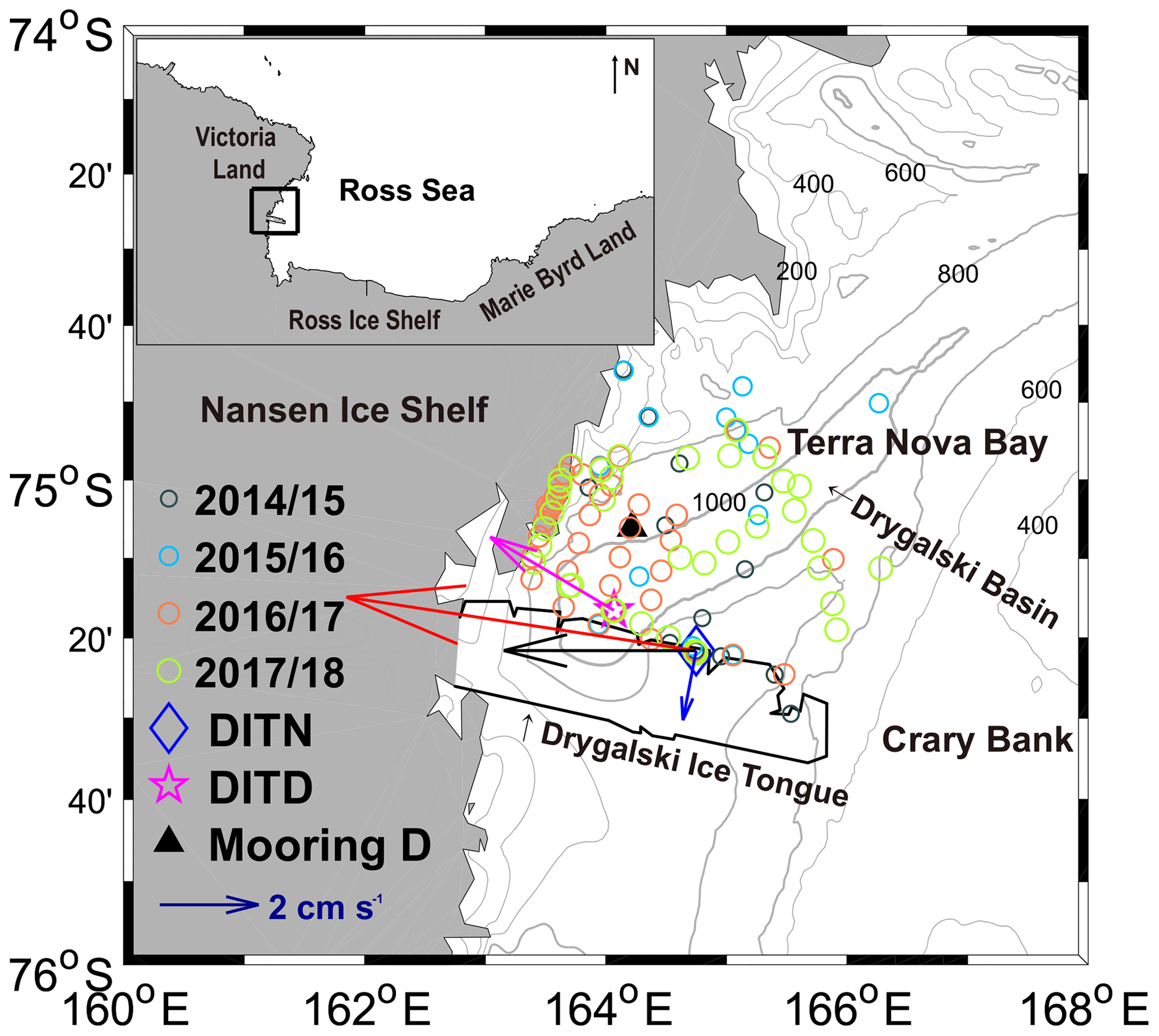
Figure 1 A topographic map of Terra Nova Bay (TNB). The location of TNB in the Ross Sea is shown in the upper left inset. The bold gray line indicates the 1000 m isobaths, and the interval between the thinner gray lines is 200 m. Conductivity–temperature–depth (CTD) stations in the austral summers (i.e., 2014, 2015, 2017, and 2018) are denoted by open circles. The averaged current vector from August to November at 660 m in the eastern TNB (DITN) (1222 m in the Drygalski Basin, DITD) is denoted by a blue (magenta) arrow. The red (black) arrow indicates the mean current vector from June to November at 75 m (273 m) in the DITN. The blue arrow in the bottom left indicates the reference velocity (2 cm s⁻¹).

This study combines ship-based in situ data collected in the austral summer (December–March) and instrumented mooring data collected in the DB and eastern TNB during December 2014–March 2018 to explore sub-polynya-scale (tens of kilometers) dynamics. In particular, we seek to answer the following research questions: (1) how does the nature of the circulation in TNB influence HSSW variation? (2) Is there any difference between the salinity variation in the western (nearshore) and eastern (offshore) parts of TNB? (3) Does katabatic wind variability play an important role in salinity variation? We then propose a sequence of typical mechanistic scales for HSSW production.

2 Data and methods

2.1 Hydrographic measurements

We examined the spatiotemporal variations in HSSW production using time series data from mooring stations in the eastern TNB (DITN) and the deepest depth level of the DB (DITD) (Fig. 1). Time series of water temperature, salinity, pressure, and ocean currents at three depths were measured using SBE37SM (Sea-Bird Scientific, Bellevue, WA, USA), RCM9 (Xylem, Inc., Rye Brook, NY, USA), and Aquadopp (Nortek, Norway) current meters attached to the DITN mooring (Fig. 2 and Table 1). The DITN mooring has been continuously maintained with annual turnarounds since December 2014 (Table 1). During the second leg of the DITN, the pressure sensor of the deepest SBE37SM failed, necessitating that a nominal sensor depth of 660 m be used. The DITD mooring was deployed at the 1230 m isobath for a single year during February 2017–March 2018, with instruments below 1200 m (Fig. 2 and Table 1). The DITN and DITD are located 32 km southeast and 20 km south of mooring D, respectively (Fig. 1). Mooring D was deployed near the NIS from 1995 to 2007, performing observations of various ocean variables at depths of up to 1000 m for 13 years (Rusciano et al., 2013).

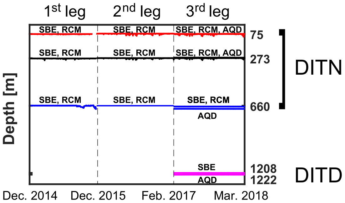
Figure 2 The recorded sensor depths during the three observation legs. The red, black, and blue lines show the depth time series for sensors at the upper, middle, and deep layer of the DITN. A magenta line also shows the recorded sensor depths of the DITD. The SBE, RCM, and AQD represent the SBE37SM, RCM9, and Aquadopp current meters, respectively (see details in Table 1).

Table 1 Information from the four oceanographic surveys and data from the DITN and DITD. U, V, T, C, and P represent the east–west current speed, north–south current speed, temperature, conductivity, and pressure, respectively. S, R, and A are the instrument abbreviations for the SBE37SM, RCM9, and Aquadopp current meters, respectively.

The temperature and salinity parameters obtained from two moorings (DITN and DITD) were validated and corrected with conductivity–temperature–depth (CTD) casts before recovery and after deployment. The salinity time series contains the short-term fluctuations induced by tidal motions and ocean currents such that the magnitude of the salinity change suggested in Sect. 3.3 was calculated after applying a 160 h (∼7 d) low-pass filter to the time series using a sixth-order Butterworth filter. The horizontal current direction was corrected for the magnetic declination. Current data collected with the RCM9 at the DITN were used for consistency of the data analysis, except for the uppermost current data of the third leg of the DITN. Current data from the RCM9 at 75 m were recorded until 1 August 2017; thereafter, an Aquadopp current meter was used. The mean differences in the current direction (speed) between observed data from the RCM9 and Aquadopp current meters at 75, 273, and 660 m were 2, 3, and 8^∘ (1.8, 0.2, and −1.2 cm s⁻¹), respectively, during the third leg of the DITN. The velocities were averaged monthly to investigate the mean advection speed and direction on monthly and seasonal timescales.

Full-depth CTD profile measurements were conducted in December 2014, December 2015, January–February 2017, and March 2018 (Table 1) aboard the ice-breaking research vessel ARAON (Korea Polar Research Institute, KOPRI). The profiles were recorded using an SBE 911 (Sea-Bird Electronics) with dual temperature and conductivity sensors. The sensor calibration dates were within 7 months of the observation dates. They were processed using standard methods recommended by SBE (Sea-Bird Electronics, Inc., 2014). The locations of CTD casts varied annually depending on sea ice and cruise priorities (Fig. 1).

To directly compare this study with results from previous studies (Budillon and Spezie, 2000; Budillon et al., 2002, 2011; Orsi and Wiederwohl, 2009), we used the practical salinity scale, rather than results based on the thermodynamic equation of seawater, i.e., TEOS-10 (McDougall and Barker, 2017). The practical salinity is smaller than the absolute salinity by about 0.17 in TNB. Potential densities (σ_θ) over 28 kg m⁻³ were used as criteria for the properties of the HSSW to distinguish the HSSW from TNB ice shelf water (TISW). TISW is characterized by its potential temperatures being lower than the freezing point at the surface ($\mathit{\theta }<-\mathrm{1.93}{}^{\circ }\mathrm{C}$) and a salinity of approximately 34.73 (Budillon and Spezie, 2000). TISW is the product of mixing between meltwater from ice-shelf melting and HSSW (Rusciano et al., 2013).

Vertical profiles of horizontal currents (5 m depth interval) were measured using a lowered acoustic Doppler current profiler (LADCP) attached to the CTD frame. The LADCP data were processed (Thurnherr, 2004) and velocities lower than the error velocity were excluded. The error velocity indicates uncertainty in the velocity estimated using the LADCP profile (Thurnherr, 2004). In addition, the horizontal currents were de-tided using all 10 available tidal components from the CATS2008 (Circum-Antarctica Tidal Simulation) model (Padman et al., 2002). The mean speeds of tidal currents during each survey were 1.0, 1.8, 0.7, and 0.7 cm s⁻¹, which were weaker than the velocities observed from the moorings and LADCP. The mean tidal ranges during each survey were 0.22, 0.45, 0.20, and 0.17 m.

2.2 Wind and sea-ice data

Hourly time series of wind and air temperature (2014–2018) recorded at the automatic weather station (AWS) Manuela (Ciappa et al., 2012; Fig. 3) were used to investigate katabatic winds blowing over TNB and estimate the sensible heat flux. The AWS Manuela is managed by the Automatic Weather Station Program of the Antarctic Meteorological Research Center at the University of Wisconsin–Madison. A katabatic wind event is defined as a period in which the wind direction is between 225 and 315^∘ (westerly) and the wind speed exceeds 25 m s⁻¹. The AWS Manuela is located within the main pathway of the katabatic winds along Reeves Glacier, making it the best option to detect the katabatic winds over TNB (Ciappa et al., 2012; Sansiviero et al., 2017).

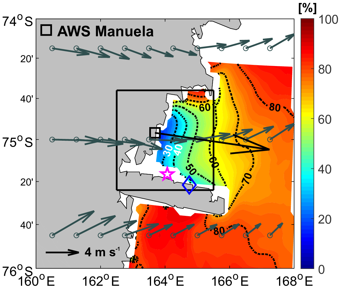
Figure 3 Spatial distributions of averaged sea-ice concentrations from July 2014 to March 2018. The interval of the dotted contour lines is a concentration of 10 %. The black square indicates the automatic weather station (AWS) Manuela. The blue diamond and magenta star are for the DITN and DITD. The dark gray and black arrows are mean wind vectors for July 2014–March 2018 using ERA-Interim data and data from AWS Manuela, respectively. The black box denotes the region over which the sea-ice concentrations are averaged in Fig. 9.

Time series of the wind and air temperature at heights of 10 and 2 m, with an interval of 3 h and a grid size of $\mathrm{0.75}{}^{\circ }\times \mathrm{0.75}{}^{\circ }$, provided by the ERA-Interim reanalysis dataset (Dee et al., 2011) were used to identify atmospheric conditions in TNB from January 2014 to March 2018 (Fig. 3). The averaged wind at the AWS Manuela was approximately 4 times faster than that provided by the ERA-Interim reanalysis data, but its direction was nearly identical to that at the grid located near Manuela (an approximately 6^∘ difference) (Fig. 3). ERA-Interim is a spatially smoothed product with a grid that is generally too coarse to resolve steep glacial slopes, which may be the reason for the large difference in wind speed compared to the observed data (Fusco et al., 2002; Dee et al., 2011). However, variations in the westerly ($\mathrm{225}{}^{\circ }\le \mathit{\theta }\le \mathrm{315}{}^{\circ }$) wind speed at Manuela had a significant correlation (99 % confidence level) with ERA-Interim retrieved values from TNB from July 2014 to March 2018 (correlation coefficient, (r)>0.70). Westerly winds detected at the Manuela station were similar to the wind in all regions of TNB in terms of the occurrence and speed variability, despite slower offshore wind speeds (Fig. 3). In this paper, all significant r values have a 99 % confidence level.

For sea-ice concentrations, we use the daily product from the Arctic Radiation and Turbulence Interaction Study with a grid spacing of 3.125 km resolved from the Advanced Microwave Scanning Radiometer 2 dataset (Spreen et al., 2008). The selected data period was from July 2014 to March 2018 in a domain within the McMurdo Sound (Fig. 3). We applied the same continental masking obtained from recent data and defined regions of sea-ice concentrations below 20 % as open water (Parkinson et al., 1999; Zwally et al., 2002). Finally, the topographic data were derived from the International Bathymetric Chart of the Southern Ocean.

3 Results

3.1 Near-bed salinity variations in TNB

Salinity observed at the deepest sensor (660 m) at the DITN mooring located in the eastern TNB (Fig. 1) exhibited interannual variations during 2015–2017 (Fig. 4a) and increased from 34.80 to 34.85. The annual cycle of salinity begins to increase from September (Fig. 4a), in association with which the change in salt contents (Fusco et al., 2009) is estimated as 2.84, 7.64, and 5.23 $\mathrm{\mu }\mathrm{g}\mathrm{salt}{\mathrm{m}}^{-\mathrm{3}}{\mathrm{s}}^{-\mathrm{1}}$ (0.007, 0.019, and 0.013 psu per month) from September to October during 2015, 2016, and 2017, respectively. Southward currents were observed when the salinity increased at the corresponding depth (Fig. 4b). The mean current direction was southwestward (191^∘), with a mean speed of approximately 1.5 cm s⁻¹ during the August–November period over the 3-year study period (Fig. 1).

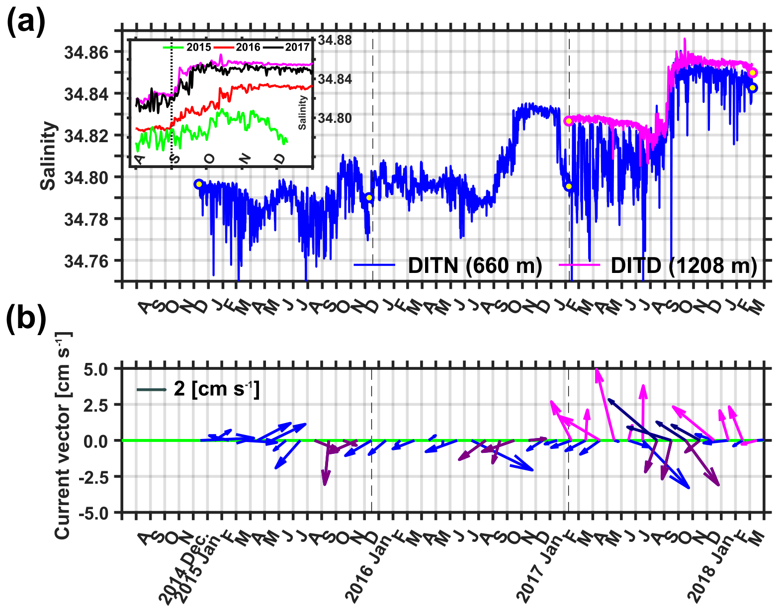
Figure 4 (a) Time series of the near-bed salinity observed in the DITN (blue) and DITD (magenta) from December 2014 to March 2018. The blue (magenta) circles filled with yellow indicate the averaged salinity in a 5 m layer at the bottom obtained using CTD data collected near the DITN (DITD). The black dashed line divides periods of each leg in the moorings (see details in Table 1). A zoomed-in plot for the 1 d moving average near-bed salinity time series from August to December of each year is shown in the small upper left inset. The magenta time series in the inset is also for the DITD. (b) Monthly mean current vectors at 660 m in the DITN and 1222 m in the DITD are indicated by blue and magenta arrows. Mean current vectors from August to November in the DITN and DITD are emphasized using purple and navy arrows, respectively.

Consistent salinity variation was observed at the other mooring (DITD) located in the DB (Figs. 1 and 4a). The salinity in the deepest part of TNB also begins to increase from September, and the salt change from September to October 2017 is estimated as 6.66 $\mathrm{\mu }\mathrm{g}\mathrm{salt}{\mathrm{m}}^{-\mathrm{3}}{\mathrm{s}}^{-\mathrm{1}}$ (0.017 psu per month) (Fig. 4a). The maximum salinity measured at the DITD is larger (∼0.006) than that at the DITN (Fig. 4a). In contrast to those observed at the DITN, northwestward currents are observed at a similar depth of salinity as that from the DITD (1222 m) during the observation periods (Fig. 4b). The mean direction of the current is northwestward (300^∘), and its mean speed is approximately 3.0 cm s⁻¹ during August–November 2017 (Fig. 1).

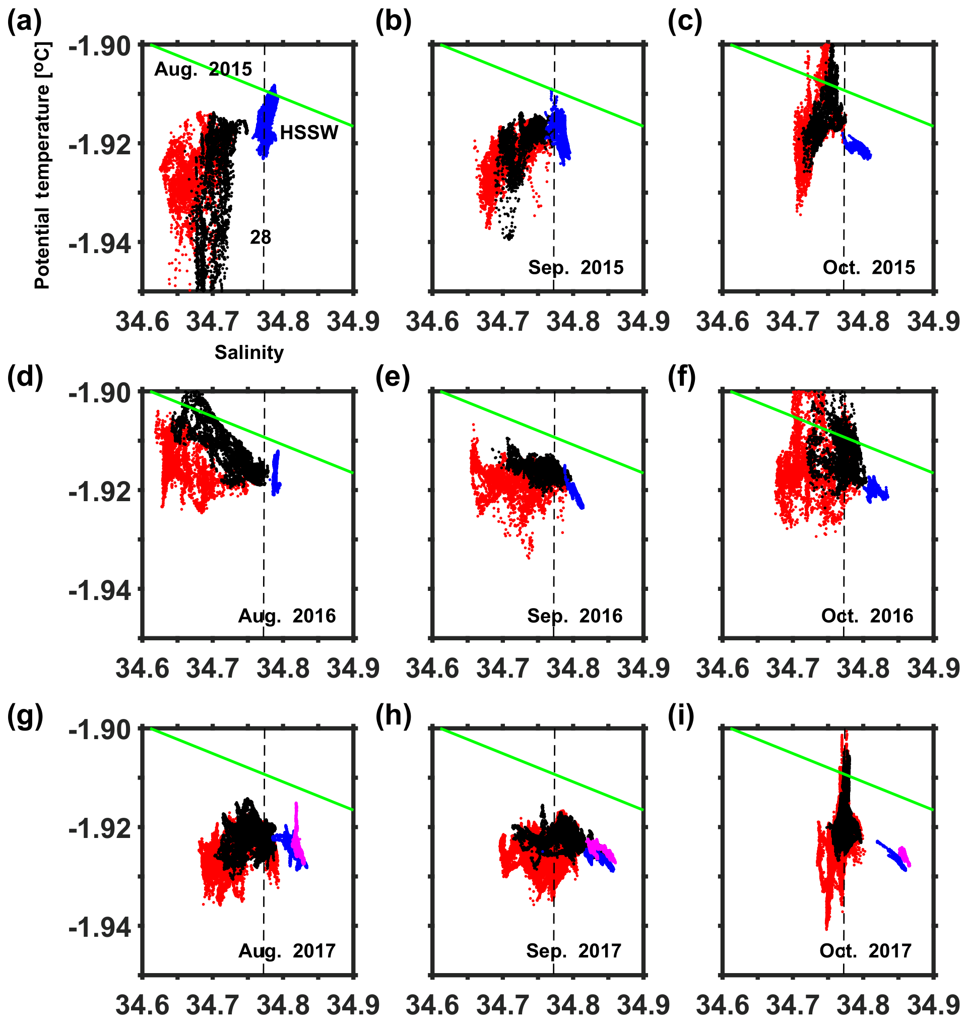
Figure 5 (a) A magnified version of the θ–S (potential temperature–salinity) diagram for data from the DITN and DITD in August 2015. Red, black, and blue dots are θ–S at 75, 273, and 660 m, respectively. The thin green line denotes the freezing point at the surface depending on the salinity, while the black dashed line indicates σ_θ=28.00 kg m⁻³. (b) The same as Fig. 5a, but for September 2015. (c) The same as Fig. 5a, but for October 2015. (d–f) The same as Fig. 5a–5c, but for August–October 2016. (g–i) The same as Fig. 5a–c, but for August–October 2017. Magenta dots are θ–S at 1208 m.

Seawater properties (temperature and salinity) observed from the DITN and DITD during August–October correspond to the HSSW properties (Fig. 5), so the relatively large changes in salt during 2016 and 2017 are an indication of active HSSW formation during the austral winter in TNBP. Evidence of HSSW formation from April to October of 2016 and 2017 was still observed 3 to 5 months later, in January 2017 and March 2018, respectively (Fig. 6). The maximum salinity in the HSSW during January–February 2017 (2016/17) and in March 2018 (2017/18) was close to those observed in the preceding October in 2016 and 2017, respectively (Figs. 4a and 6). The mean salinity in the HSSW (${\mathit{\sigma }}_{\mathit{\theta }}>\mathrm{28}\mathrm{kg}{\mathrm{m}}^{-\mathrm{3}}$) was also calculated as 34.788 (σ=0.002), 34.785 (0.005), 34.801 (0.009), and 34.815 (0.016) for each survey.

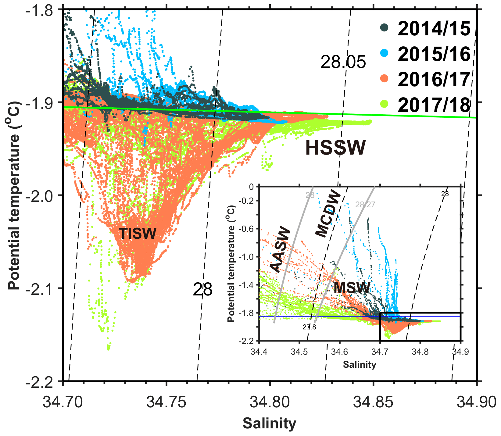
Figure 6 A zoomed-in plot of the θ–S diagram for CTD data collected in TNB during each observation period. The solid green line denotes the freezing point at the surface depending on the salinity, and the black dashed lines indicate isopycnals. The full-range θ–S diagram is shown in the inset. The black box and blue line in the inset indicate the ranges of the magnified plot and the −1.85 ^∘C isotherm, respectively. The gray solid lines denote 28 and 28.27 kg m⁻³ neutral density (γⁿ) surfaces. AASW, MCDW, MSW, TISW, and HSSW represent Antarctic Surface Water, modified Circumpolar Deep Water, modified shelf water, Terra Nova Bay ice shelf water, and high-salinity shelf water, respectively.

Vertical profiles of salinity and potential density also had features consistent with the θ–S diagram (Fig. 7). The properties in a quasi-homogeneous bottom layer below 800 m (Fig. 7) represent the properties of HSSW formed just before the austral winter. The salinity of this layer was relatively high in the 2016/17 and 2017/18 surveys (Fig. 7a; peak salinities of 34.83 and 34.85, respectively) and was similar to that observed in the early 2000s when HSSW transport was relatively large (>1.2 Sv) in TNB during 1995–2006 (Fig. 7a; Fusco et al., 2009).

Figure 7 (a) Vertical salinity profiles at each observation period. The black solid line indicates 34.8. The asterisks indicate salinity at ∼900 m of depth in TNB observed during 1995–2006 from Fusco et al. (2009) (b) The same as Fig. 7a, but for potential density (σ_θ); the black solid line indicates 28.0 kg m⁻³.

3.2 Upper-ocean salinity variations in the eastern TNB

Salinity in the upper water column of the eastern TNB shows a more distinct seasonal variation compared to the salinity at 660 m (Fig. 8a). The salinity at both 75 and 273 m decreased, while the salinity at 75 m decreased to below 34.0 in February of each year (Fig. 8a). Thereafter, the salinity of the two layers started mixing, as the salinity increased at 75 m and decreased at 273 m. The salinity at both depths then increased in tandem until September (Fig. 8a). Note that the vertically well-mixed period gets longer over the 3 years. The well-mixed period, defined as a period in which the difference in σ_θ between the two layers is less than 0.1 kg m⁻³ (Dong et al., 2008), was initiated in early May 2015, at the end of April 2016, and in early April 2017 (Fig. 8b). In December, the mixing of the two layers ceases, and their salinity difference becomes larger again (Fig. 8a). The restratification is due to changes in buoyancy as a result of ice melting at the surface during the austral summer.

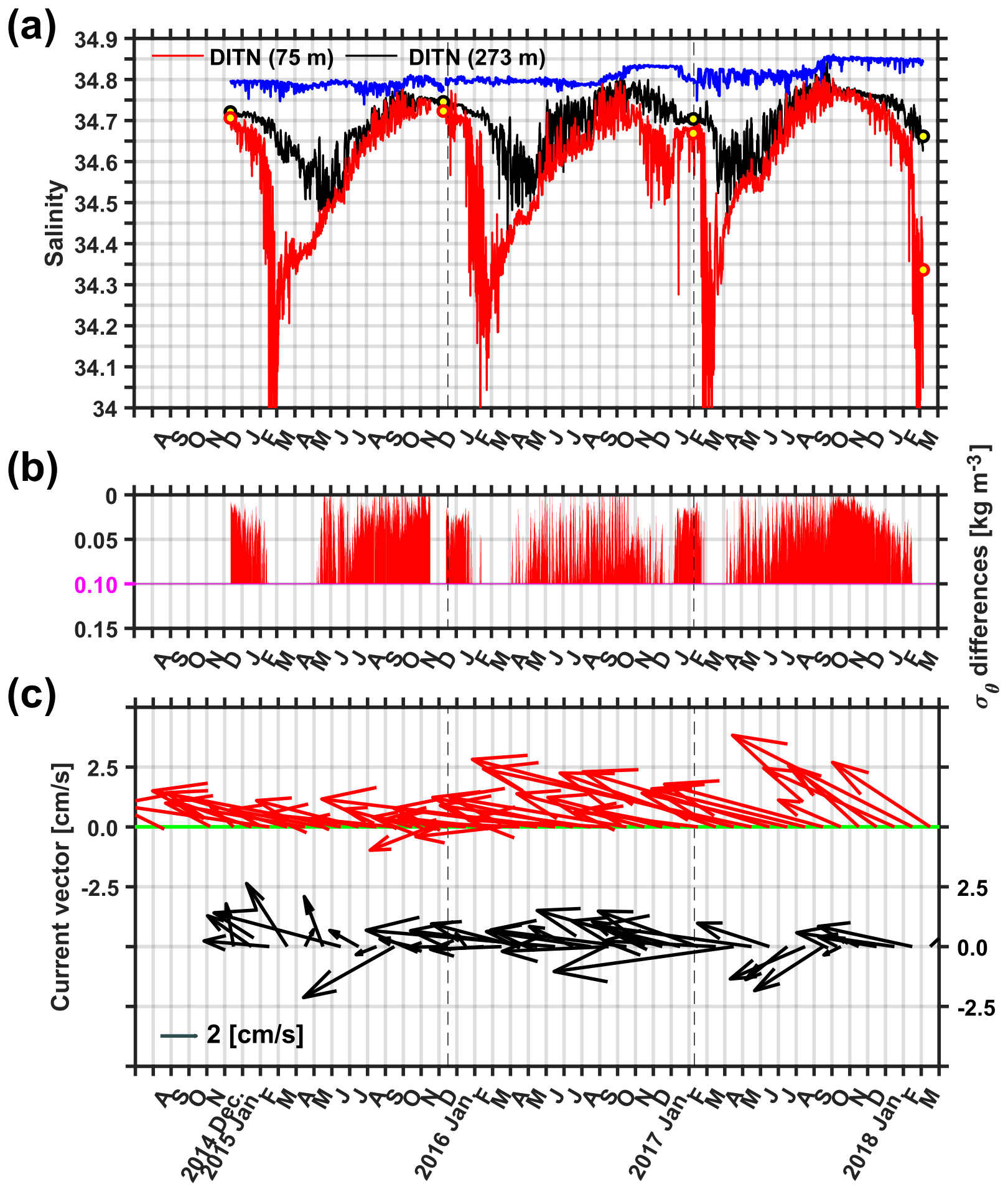
Figure 8 (a) Salinity time series at three depths from the DITN. The red (black) circles filled with yellow are the averaged salinity in a 5 m layer at 75 m (273 m) obtained using CTD data collected near the DITN. The black dashed line divides periods of each leg at the moorings (see details in Table 1). (b) Potential density (σ_θ) differences lower than 0.10 kg m⁻³ for σ_θ at 75 and 273 m are shown. The magenta line indicates a 0.10 kg m⁻³ difference. (c) Monthly mean current vectors at 75 and 273 m of the DITN are indicated by red and black arrows.

The maximum salinity observed at depths of 75 and 273 m during September–October also increased from 2015 to 2017 (34.774, 34.804, and 34.849, respectively), which is consistent with the trend of maximum salinity observed at deeper depths as presented in the previous subsection (Figs. 4a, 6, 7, and 8a). Water properties corresponding to the HSSW were detected even in the upper parts during the months of August to October in 2016 and 2017 (Fig. 5d–i), suggesting that the HSSW can be locally formed through convective processes in the eastern TNB. The averaged salinity in the upper water column during September–October in 2016 and 2017 was lower (∼0.05) than that observed at 660 m (Figs. 5 and 8a), so it is not responsible for the salinity increase at the near-bed level of the eastern TNB (Fig. 4a). In contrast, HSSW formation was rarely observed from August to October 2015, when the increase in salinity was relatively small compared with the increases during the same period in 2016 and 2017 (Figs. 4a and 5a–c).

During December 2014–March 2018, westward currents were dominant at the two depths (Fig. 8c), with an average current speed (direction) from June to November of 7.4 cm s⁻¹ (279^∘, westward) at 75 m and 4.0 cm s⁻¹ (270^∘, westward) at 273 m (Fig. 1). The westward currents suggest that the upper water column of the DITN was affected by seawater advected from the eastern part of TNB.

3.3 The role of wind in TNBP

The wind in TNB is primarily westerly, which on average creates an L-shaped polynya along the NIS and DIT, as shown by the contour line that represents a sea-ice concentration of 50 % in Fig. 3. Westerly winds at Manuela effectively opened TNBP during the austral winters (April–October) of the 3-year study period (Fig. 9). The daily wind speed and the percentage of open water during the austral winter are significantly correlated (r=0.46) during 2015–2017 (Fig. 9). In the austral winter during each year, r was 0.49, 0.50, and 0.37, respectively, and all values were significant.

Katabatic wind events most frequently occurred from April to October 2017 (210 events) at Manuela station. The mean duration of a single katabatic wind event during these 7 months in 2015, 2016, and 2017 was 6.5, 7.0, and 7.7 h, respectively. Moreover, the average length of time for which the polynya was open (i.e., >20 % open water in Fig. 9) during the same periods was 5.8 d (2015), 6.7 d (2016), and 7.7 d (2017). In short, the polynya opens for a longer time period with more persistent katabatic winds during the 2017 austral winter than during the other 2 years.

From June to September of 2016 and 2017, a footprint of HSSW production via convective processes was found in the upper water column in the eastern TNB (Fig. 8a). This indicates that katabatic winds – considered vital to the development of a polynya (Fig. 9) – induce convection by a supply of brine related to new ice production in the eastern polynya. The total magnitude of the salinity increase during the katabatic wind events from June to September was the largest in 2017 at both 75 and 273 m among the 3 years. At 75 m (273 m), salinity increases of 0.082, 0118, and 0.120 (0.065, 0.050, and 0.142) were observed in 2015, 2016, and 2017, respectively. Salinity increases due to katabatic wind events accounted for 54 % and 76 % of the total salinity increase observed at 75 and 273 m during June–September in 2017.

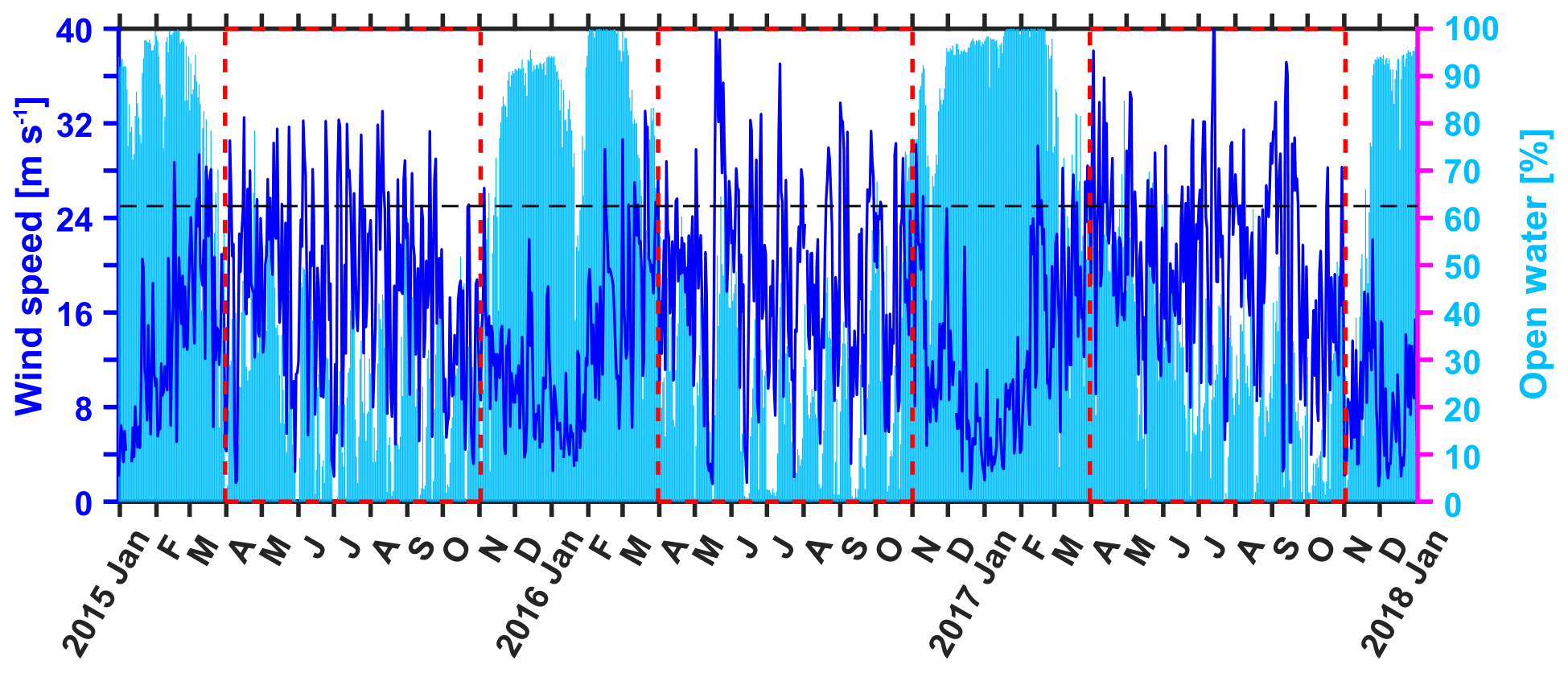
Figure 9 Time series from 2015 to 2017 for daily westerly ($\mathrm{225}{}^{\circ }<\mathit{\theta }<\mathrm{315}{}^{\circ }$) wind speeds from Manuela (blue line), as well as the daily percentage of open water averaged from the black box shown in Fig. 3 (sky blue bar). Red dashed boxes indicate a time period from April to October. The black dashed line indicates a wind speed of 25 m s⁻¹.

4 Discussion

Despite being a small, confined polynya, TNBP generates a substantial proportion of the global AABW. Understanding the supply of HSSW, and ultimately AABW, requires a focus on small-scale processes from a regional perspective. Here, we investigate the evolution of HSSW in TNB through the spatiotemporal variations in salinity observed in the eastern TNB and DB.

4.1 Present data in the context of previous analyses

Data from mooring D (Fig. 1) in TNBP show seasonal variation in the stratification of the water column and interannual variation in the HSSW properties, which are closely associated with polynya activity (Rusciano et al., 2013). This implies that HSSW production occurs during the austral winter, and favorable katabatic wind events control the properties of the HSSW.

Data gathered for this study have revealed that the HSSW can also form at the surface of the eastern TNB. The salinity (density) variations in the upper layers at the DITN exhibit HSSW formation in the polynya via convection led by a supply of brine from the surface, as suggested by modeling studies on TNBP (Fig. 8a; Buffoni et al., 2002; Mathiot et al., 2012). Water masses farther away from TNB are less saline due to mixing with the CDW or the intrusion of MCDW into the western Ross Sea (Fusco et al., 2009; Orsi and Wiederwohl, 2009; Budillon et al., 2011), so the advection of seawater from the eastern part of TNB (Fig. 8c) would hardly contribute to the salinity increase in the upper water column of the DITN.

In addition, we found that large salinity increases (>0.04), related to active HSSW formation, were observed in the deepest part of the DB and eastern TNB from September to October (Fig. 4a); however, the salinity increase was observed at the DITN and DITD approximately 1–2 months later than at mooring D. The salinity observed at 550 m at mooring D increased since the beginning of July due to HSSW production (Rusciano et al., 2013). Rusciano et al. (2013) suggested that HSSW formed near the NIS advected towards the center of TNB along the 800–1000 m isobaths. Therefore, the salinity increase from September at the DITN and DITD (Fig. 4a) would be due to HSSW advection from the NIS but not from the sinking of HSSW directly from the surface at the mooring locations.

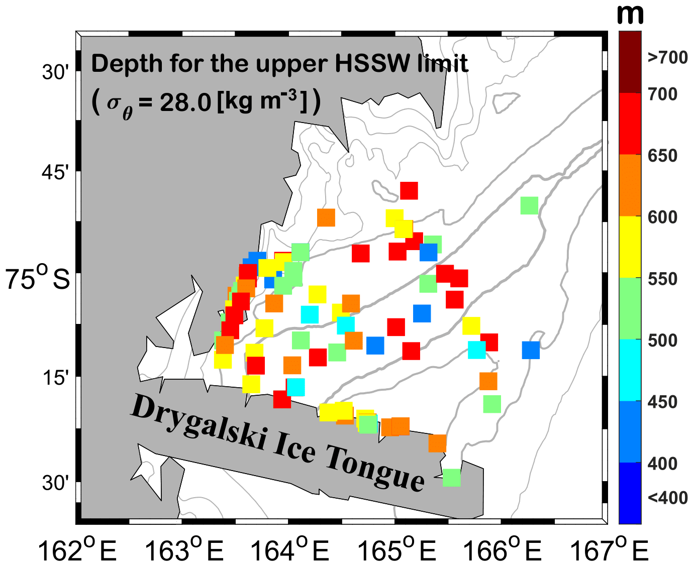
Figure 10 Distributions of depth (m) for the upper HSSW limit (σ_θ=28 kg m⁻³) in vertical CTD profiles during the four hydrographic surveys (see details in Table 1). The bold gray line indicates the 1000 m isobaths and the interval between the thinner gray lines is 200 m.

The HSSW formed in the austral winter arrives at the deepest part of the DB and eastern TNB within a few months. Thus, the HSSW is evenly distributed over TNB during the austral summer (Fig. 10). The depths for the upper HSSW limit (σ_θ=28 kg m⁻³) are within a range from 400 to 700 m over TNB (Fig. 10), so the HSSW occupies a 500–800 m water column from the seabed in the austral summer. In addition, the average salinity of the HSSW in the eastern part at 164.5^∘ E (34.802) shows no difference from that in the western part at 164.5^∘ E (34.802) during the CTD observation periods. According to vertical sections of salinity from the 2017/18 survey, the salinity in the deep layer (>600 m) was nearly identical between the western and eastern part of TNB (Fig. 11a), with a distributed salinity over 34.80 at greater depths (>800 m) of the DB (Fig. 11b). In the upper parts of the HSSW (σ_θ<28 kg m⁻³), modified shelf water and Antarctic Surface Water were dominantly distributed over TNB during the austral summer (Fig. 11). Water properties corresponding to the MCDW were rarely seen for the austral summer (Figs. 6 and 11), implying that MCDW's effect on salinity changes throughout TNB seems to be limited.

Figure 11 (a) Vertical section of salinity along the Drygalski Ice Tongue (blue-filled squares in the inset) observed during the 2017/18 survey. The color bar for salinity is denoted in Fig. 11b and its interval is 0.01. The black contour lines indicate isopycnals (kg m⁻³). AASW, MSW, and HSSW represent Antarctic Surface Water, modified shelf water, and high-salinity shelf water, respectively. (b) The same as Fig. 11a, but for the section along the Drygalski Basin (red circles in the inset of Fig. 11a).

Furthermore, the role of wind in TNBP was investigated by statistics of katabatic winds during 2015–2017. We showed that the number of katabatic wind events was the largest in the 2017 austral winter (April–October) among the 3 years. The mean duration of katabatic wind events and the mean time for which the polynya was open were also the longest during the austral winter of 2017. The longer the polynya is exposed to wind, the more heat would be removed from the water column. Thus, these results support more active formation of the HSSW in 2017 than in 2015 and 2016 (Figs. 6 and 7). The upper-ocean salinity increases estimated during the katabatic wind events of each year also suggest that more brine was released from ice formation during more persistent katabatic winds in 2017 and contributed to a larger salinity increase in the upper water column in the eastern TNB and to local HSSW formation. Rusciano et al. (2013) have suggested that HSSW formation is more dependent on the duration of a single katabatic wind event than on its frequency during the austral winter. However, for the 3-year study period, both the duration and frequency of katabatic wind events are important factors for active HSSW formation in TNBP.

4.2 Circulations in TNBP

For the austral summer (December–March), westward currents flowing along the DIT and northward currents flowing along the NIS were observed based on the de-tided LADCP current data averaged over a depth range of 400–700 m (Fig. 12a). The currents resemble a cyclonic pattern together with the southeastward currents in the northeastern TNB, despite southward currents that flow toward the DIT (Fig. 12a). The current speed is relatively weaker at the center of the DB than in other TNB regions, and southeastward currents that cross over from the NIS to the DIT were not observed.

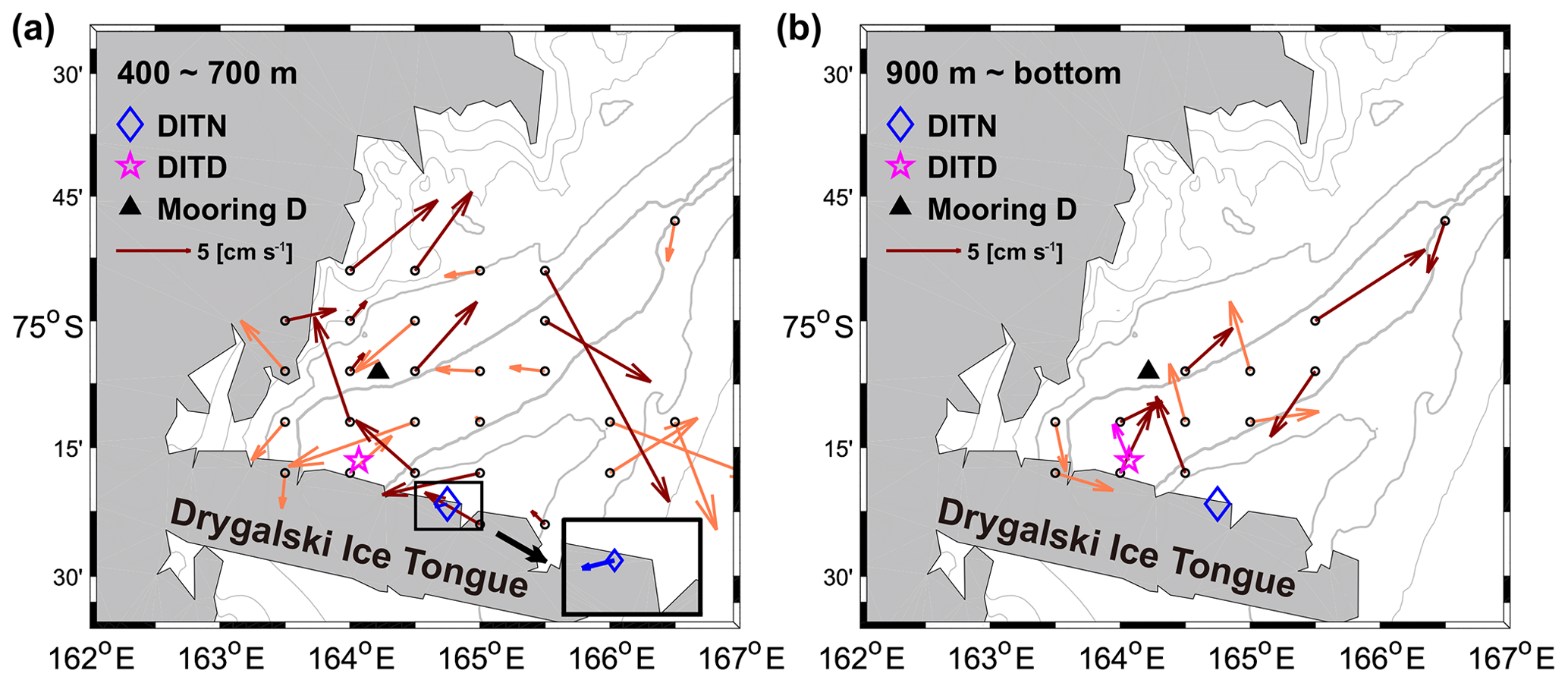
Figure 12 (a) Mean currents in a range of 400–700 m during four hydrographic surveys (see details in Table 1). The LADCP data are arranged by averaging the data on a ${\mathrm{0.5}}^{\circ }\times {\mathrm{0.1}}^{\circ }$ grid. The averaged current vector from January to February at 660 m in the DITN is denoted by a blue arrow. The inset shows the current vectors of the DITN. The current vectors mainly discussed in Sect. 4.2 are highlighted by dark red. The bold gray line indicates the 1000 m isobaths, and the interval between the thinner gray lines is 200 m. A scale arrow is denoted in the left part of the figure. (b) The same as Fig. 12a, but for the range of 900 m–bottom. A magenta arrow shows the averaged current vector from January to February at 1222 m in the DITD.

The wind-driven cyclonic gyre in the upper layer of TNBP (van Woert et al.,  2001) may induce an upwelling in the center of TNB, so it would hinder the development of horizontal flows in the central region of the gyre. The upwelling feature is visible in the vertical sections of the 2017/18 survey as upward-bending isopycnals in the upper layers (>400 m) of the midpoint of TNB (Fig. 11b). Similarly, depths for the upper HSSW limit seem to be shallower in the center of TNB than other regions of TNB (Fig. 10).

If we assume that the circulation pattern was maintained throughout the year, then the HSSW formed near the NIS would circulate clockwise rather than directly flowing southeastward toward the DITN. The southward currents observed at 660 m at the DITN mooring during periods of the salinity increase (Fig. 4b) would also be thought of as the southern rim of the cyclonic circulation in TNB. Thus, we can conclude that the deep salinity in the eastern TNB has increased since September due to the advection of HSSW originating from the NIS. In addition, the reason why the salinity increase at the DITN occurs later (1–2 months) than at mooring D is that the HSSW flows along the cyclonic circulation. The distance from the DITN to mooring D is so short (∼32 km) that a water parcel from mooring D can arrive at the DITN within 13 d with average 3 cm s⁻¹ southeastward currents.

As HSSW salinity observed at the DITD is larger than that at the DITN (Fig. 5g–i), the salinity increase at the DITD (Fig. 4a) is not related to the northwestward HSSW advection from the eastern TNB along the cyclonic circulation (Fig. 12a). The near-bed ocean currents in the DB flow under the influence of gravity (Jendersie et al., 2018); however, it is still unclear how the HSSW at greater depths circulates around the DB. The LADCP data for December–March might provide an indication of the circulation in the deeper parts of the DB (>1000 m) because the current direction at the DITD remains approximately northwestward for about 1 year (Fig. 4b).

The southwestward currents appear in the northeastern part of the DB, while the northwestward and northeastward currents appear in the southern and western region of the DB, according to the currents averaged from 900 m to the seafloor during the austral summer (Fig. 12b). The currents resemble an abyssal cyclonic circulation confined within the DB, not the upper cyclonic circulation in TNB (van Woert et al., 2001). The northwestward current observed at 1222 m at the DITD mooring during the salinity increase period (Fig. 4b) is considered to be a part of the abyssal circulation, thus suggesting that the HSSW flowing into the DB from the NIS circulated cyclonically in this region and can be detected at the sensors of the DITD mooring from September to October. The DB is an export pathway for HSSW formed in the Ross Sea polynya and TNBP, so the circulation pattern in this region requires further investigation by acquiring more in situ ocean current data and ocean circulation model developments.

4.3 Characteristics of the TISW

The TISW, which is colder than −1.93 ^∘C, was observed at depths between 300 and 600 m in January–February 2017 (2016/17) and March 2018 (2017/18) but was not observed during December surveys (2014/15 and 2015/16) (Figs. 6 and 13a). It seems that the TISW was formed when the HSSW was actively produced in TNB (Fig. 6); however, the presence of the TISW is dependent on the observation period. For example, the TISW becomes colder (∼0.05 ^∘C) and less saline (∼0.02) from late January (2016/17) to March (2017/18) (Figs. 6 and 13a). The TISW, with over 200 m thickness, was only found near the NIS in late January (Fig. 13b), but, in March, it was distributed from the NIS to the northeastern TNB (Fig. 13c). It seems that the TISW near the NIS advects with the cyclonic circulation in TNB (Figs. 12a and 13c). Therefore, meltwater outflow from nearby ice shelves may occur from late January to March. Compared with the previous observations, the TISW becomes much colder (>0.1 ^∘C) than the potential temperature of the TISW observed in the late 1990s (Budillon and Spezie, 2000). The colder TISW could contribute to more sea-ice production at the surface of TNB, so the characteristics and variability of the TISW merit further studies.

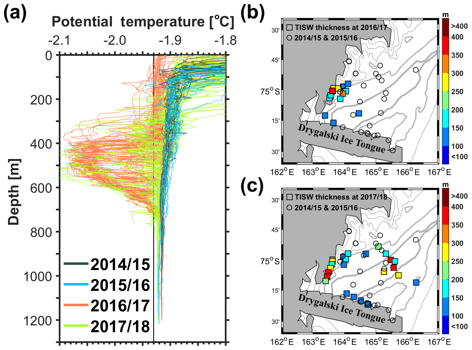
Figure 13 (a) The same as Fig. 7a, but for potential temperature; the black solid line denotes $-\mathrm{1.93}{}^{\circ }\mathrm{C}$. (b) Distributions of Terra Nova Bay ice shelf water (potential temperature $<-\mathrm{1.93}{}^{\circ }\mathrm{C}$) thickness (m) in vertical CTD profiles during the 2016/17 survey (see details in Table 1). The bold gray line indicates the 1000 m isobaths, and the interval between the thinner gray lines is 200 m. (c) The same as Fig. 13b, but for the 2017/18 survey.

4.4 Mixed-layer development in the eastern TNB

As shown in Sect. 3.2, the time in which the upper (at least to 273 m) water column becomes homogenous is the earliest in 2017 throughout the 3-year study period (Fig. 8a and b). This suggests that the salinity at the two depths was characterized by rapid mixing during March–April 2017, with a long-lasting covariation time until October 2017 (Fig. 8a). The mean wind speed (number of katabatic wind events) from March to May during 2015, 2016, and 2017 was calculated as 18.6, 20.2, and 21.0 m s⁻¹ (74, 85, and 96), respectively. These wind statistics indicate that wind-driven mixing (mechanical mixing between two layers) was the strongest between March and May 2017. Thus, katabatic winds would also play a role in mixed-layer development before inducing HSSW production through the convective process in the eastern TNB. However, the magnitude of the salinity increase at 75 m was much larger than that of the salinity decrease at 273 m during March–May of each year, so the surface buoyancy flux from heat loss and/or sea-ice production contributed more to the mixing in this period. For example, the salinity at 75 m increased over 0.5 from March to May 2017, whereas the salinity at 273 m decreased about 0.15 in the same period.

4.5 TNBP mechanical scales

HSSW produced near the NIS spreads horizontally into the eastern TNB and DB at current speeds lower than 5 cm s⁻¹ in less than 2 months (from July to September) (Figs. 1, 4, 8, and 12; Rusciano et al., 2013). If we assume that the circulation in TNBP has a radius of 25 km (approximately one longitudinal degree) (Fig. 12a), the circumference of the circulation is about 160 km. Then we can deduce that the HSSW circulates cyclonically about 80 km ($\sim \mathrm{160}/\mathrm{2}$ km) from the NIS to the eastern parts of TNB, which takes about 1 month at a current speed of 3 cm s⁻¹.

TNBP usually forms as an L shape, similar to a model-derived polynya (Sansiviero et al., 2017; Fig. 3). This indicates that the open water is predominantly formed along the coasts near NIS (DIT) for approximately 40^′ (latitudinal) over 75 km (2^∘ longitude being equivalent to 55 km). The average area for polynya activity is approximately 1300 km² ($\mathrm{75}\mathrm{km}\times \mathrm{10}\mathrm{km}+\mathrm{55}\mathrm{km}\times \mathrm{10}\mathrm{km}$) based on the assumption that the width of the open water is 10 km from the coast using the 40 % sea-ice concentration contour line (Fig. 3). This accounts for about 4 % of the sea-ice production area in the Ross Ice Shelf polynya (Cheng et al., 2017). The opening of TNBP by westerly winds that blow from across the NIS occurs over the span of a day (Fig. 9). During this time, the percentage of open water can vary by up to ±40 % (Fig. 9). The mean duration of the polynya opening is about 7 d during the austral winter in the analysis period.

4.6 Quantification of sea-ice production

The link between katabatic winds and HSSW formation can be described as follows: (i) katabatic winds move sea ice into the offshore region, (ii) the polynya opens, (iii) katabatic winds and atmospheric cooling remove the heat from the polynya, (iv) sea ice is produced in the surface, (v) brine is rejected, (vi) stratification breaks down, and (vii) HSSW accumulates. Thus, precise quantification of sea-ice production and brine formation in the polynya region is required for an in-depth understanding of HSSW formation processes. However, current data for the brine supply from sea-ice formation in the polynya provided insufficient constraints. In this part, we attempt to estimate the net heat flux from only the sensible heat flux by assuming that it is the main component for determining the net heat flux in TNB (Fusco et al., 2009). The sensible heat flux was calculated by using the AWS Manuela daily wind and air temperature data (Budillon et al., 2000), and the sea surface temperature was assumed to be near the freezing point (−1.9 ^∘C). The daily air temperature observed at Manuela was also significantly correlated (r>0.90) with ERA-Interim retrieved values from TNB from July 2014 to March 2018.

According to the calculations, the mean sensible heat flux was −178, −182, and $-\mathrm{232}\mathrm{W}{\mathrm{m}}^{-\mathrm{2}}$ during katabatic wind events from April to October in 2015, 2016, and 2017, respectively. In 2015 and 2016, sea-ice production of 32 and 33 km³ and HSSW transport of 1.6 and 1.6 Sv were estimated using the heat flux parameterization (Fusco et al., 2009). Higher sea-ice production of 42 km³ and HSSW transport of 1.9 Sv were obtained due to more sensible heat loss in 2017. The estimated sensible heat flux, sea-ice production, and HSSW transport during April–October 2017 were very similar to values in 2003 when the largest sea-ice production occurred during 1990–2006 (Fusco et al., 2009). Moreover, in January of 2004, the averaged salinity in a 10 m layer at a depth of 900 m was observed to be 34.837 (Fusco et al., 2009), which is almost the same as the value (34.838) observed in March 2018 (2017/18 survey) (Table 1). Since it is a rough estimation for sea-ice production, in situ data should be continuously collected to clarify spatial and temporal relationships among wind speed, heat flux, sea-ice production, and brine release in TNBP.

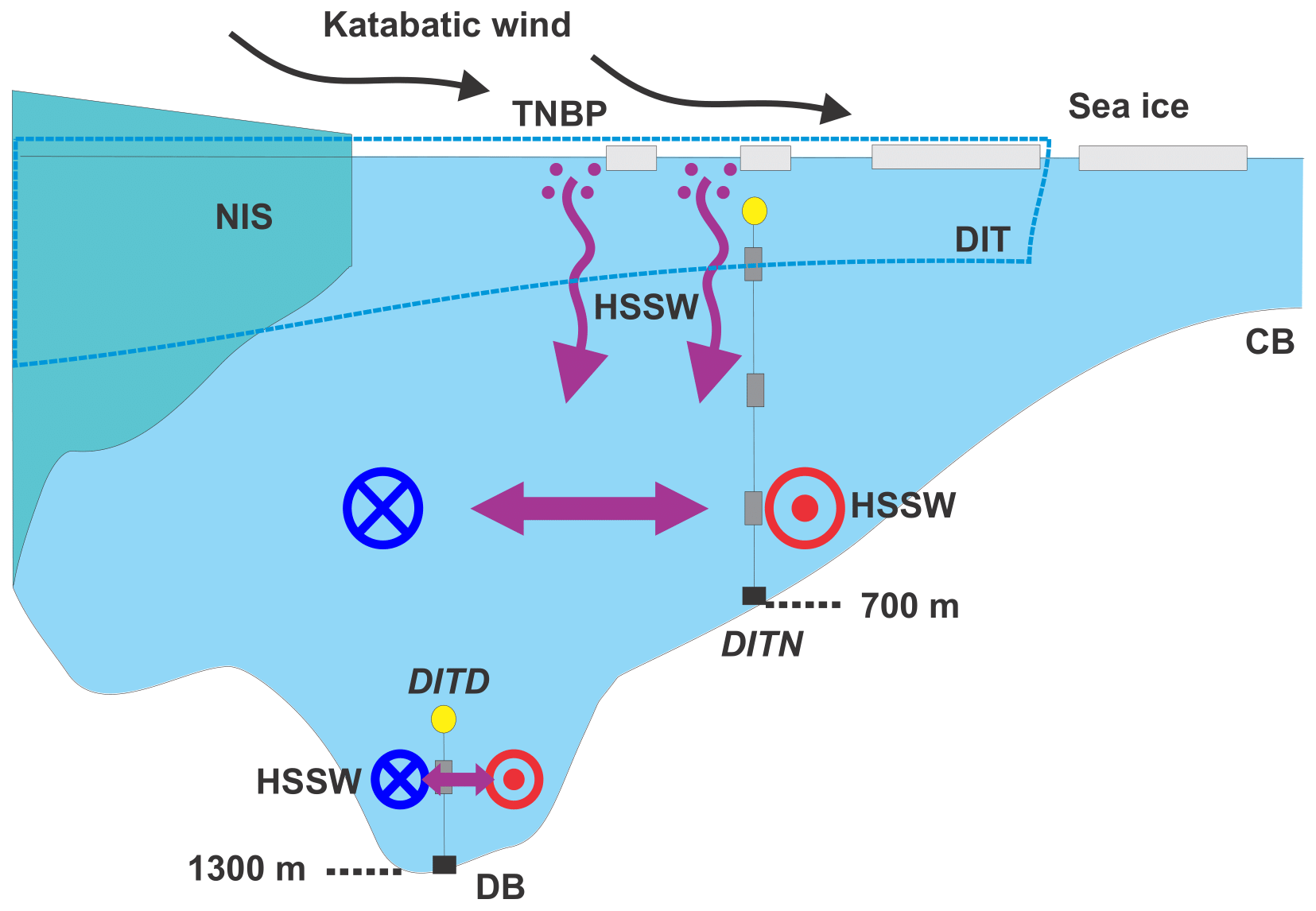
Figure 14 A schematic of the spatiotemporal variations in the production of HSSW in TNBP. The downward arrows show HSSW formation through convection from brine rejection (dots) during sea-ice formation at the surface in the polynya opened by off-shelf katabatic winds. The horizontal bidirectional arrows indicate that the HSSW that formed near the Nansen Ice Shelf (NIS) advects at the deepest depths of both the eastern Terra Nova Bay (DITN) and Drygalski Basin (DITD) via cyclonic pattern flows in TNBP. The blue and red circles represent flow into and out of the polynya. DB, CB, and DIT denote the Drygalski Basin, Crary Bank, and Drygalski Ice Tongue, respectively.

5 Conclusions

This study investigated the spatial patterns and temporal changes in HSSW formation in TNBP during a period from December 2014 to March 2018 using a comprehensive in situ observational dataset. In response to the three research questions listed in Section 1 our analyses suggest the following: (1) HSSW formed near the NIS flows cyclonically in the deeper parts of TNBP, ultimately reaching the eastern TNB from September to October (Fig. 14). The HSSW formed near the NIS also reaches the greatest depth in the DB from September to October and is horizontally distributed by the cyclonic circulation in the DB (Fig. 14). (2) The salinity increase occurs in the western (nearshore) parts of TNB first from July to September and then in the eastern (offshore) parts about 2 months later from September to October; however, there are no significant salinity differences between the eastern and western parts during the austral summer (Figs. 10 and 11). (3) The katabatic winds that blow from across the NIS drive general salinity increases and episodic HSSW formation through ice production and brine release in the upper parts of the eastern TNB (Fig. 14). These answers complement the previous results on HSSW formation in TNBP well.

Large-scale freshening of AABW sources (including HSSW) has been reported in the Ross Sea and TNB in recent decades (Jacobs et al., 2002; Fusco et al., 2009; Jacobs and Giulivi, 2010), which may be relevant to the findings presented herein. We showed higher (>0.025) salinity values near 900 m of depth in January–February 2017 and March 2018 than in December 2014 and December 2015 (Table 1), implying more active HSSW formation in TNBP that was comparable to that in the early 2000s (Fig. 7a; Fusco et al., 2009). The HSSW formed in TNB can flow off the shelf break along Victoria Land (Cincinelli et al., 2008; Jendersie et al., 2018) and potentially affect the volume or properties of AABW in the western Ross Sea. Most recently, the rebound of HSSW salinity was reported from observations in the western Ross Sea (Castagno et al., 2019). These recent findings have roughly suggested that active sea-ice formation in TNBP and the Ross Ice Shelf polynya and a decrease in freshwater input from the Amundsen Sea contribute to this salinity rebound. Also, our findings have implications for the response of the overturning circulations in the Southern Ocean to regional anomalies in buoyancy forcing (Rintoul, 2018) as local HSSW formation may significantly contribute to the response and requires additional studies.