the Creative Commons Attribution 4.0 License.
the Creative Commons Attribution 4.0 License.
 | 07 Oct 2020
Coastal sea level rise at Senetosa (Corsica) during the Jason altimetry missions
Yvan Gouzenes
Fabien Léger
Anny Cazenave
Florence Birol
Pascal Bonnefond
Marcello Passaro
Fernando Nino
Rafael Almar
Olivier Laurain
Christian Schwatke
Jean-François Legeais
Jérôme Benveniste
In the context of the ESA Climate Change Initiative project, we are engaged in a regional reprocessing of high-resolution (20 Hz) altimetry data of the classical missions in a number of the world's coastal zones. It is done using the ALES (Adaptive Leading Edge Subwaveform) retracker combined with the X-TRACK system dedicated to improve geophysical corrections at the coast. Using the Jason-1 and Jason-2 satellite data, high-resolution, along-track sea level time series have been generated, and coastal sea level trends have been computed over a 14-year time span (from July 2002 to June 2016). In this paper, we focus on a particular coastal site where the Jason track crosses land, Senetosa, located south of Corsica in the Mediterranean Sea, for two reasons: (1) the rate of sea level rise estimated in this project increases significantly in the last 4–5 km to the coast compared to what is observed further offshore, and (2) Senetosa is the calibration site for the TOPEX/Poseidon and Jason altimetry missions, which are equipped for that purpose with in situ instrumentation, in particular tide gauges and a Global Navigation Satellite System (GNSS) antenna. A careful examination of all the potential errors that could explain the increased rate of sea level rise close to the coast (e.g., spurious trends in the geophysical corrections, imperfect inter-mission bias estimate, decrease of valid data close to the coast and errors in waveform retracking) has been carried out, but none of these effects appear able to explain the trend increase. We further explored the possibility that it results from real physical processes. Change in wave conditions was investigated, but wave setup was excluded as a potential contributor because the magnitude was too low and too localized in the immediate vicinity of the shoreline. A preliminary model-based investigation about the contribution of coastal currents indicates that it could be a plausible explanation of the observed change in sea level trend close to the coast.
- Article
(7786 KB) - Full-text XML
- BibTeX
- EndNote


Since the early 1990s, satellite altimetry has provided invaluable observations of the global mean sea level and its regional variability. In recent years, this data set has generated abundant literature on the processes causing sea level change at global and regional scales, as well as on closure of the sea level budget (e.g., Church et al., 2013; Stammer et al., 2013; Dieng et al., 2017; Nerem et al., 2018; WCRP, 2018; SROCC, 2019). In addition to the global mean rise and superimposed regional trends, changes in small-scale processes, such as local atmospheric effects, baroclinic instabilities, coastal trapped waves, shelf currents, waves and fresh water input from rivers in estuaries, can substantially modify the rate of sea level change at the coast compared to open sea regions (Woodworth et al., 2019; Melet et al., 2018; Piecuch et al., 2018; Dodet et al., 2019; Durand et al., 2019). In addition, ground subsidence may amplify the rate of sea level change at the coast (Woppelmann and Marcos, 2016). In terms of societal impacts, what really matters in the coastal zone is indeed the sum of the global mean sea level rise plus the regional trends and the local processes.
Until recently, due to land contamination of radar echoes and less precise geophysical corrections, classical altimetry did not provide reliable sea level data in a band of 10–15 km along coastlines. However, different studies have shown that using adapted reprocessing of altimetry measurements and improving geophysical corrections allow the retrieval of a large amount of valid sea level data close to the coast (e.g., Cipollini et al., 2018; Passaro et al., 2015; Marti et al., 2019). In addition, despite having a much higher noise level than the classical 1 Hz altimetry data, high-resolution 20 Hz measurements allow us to recover more information on coastal sea level variations (Birol and Delebecque, 2014; Leger et al., 2019).
In the context of the Climate Change Initiative (CCI) project of the European Space Agency (ESA), we have initiated a reprocessing of high-resolution (20 Hz) altimetry data of the Jason-1 and Jason-2 missions along coastal zones of western Africa, northern Europe and the Mediterranean Sea. The ALES (Adaptive Leading Edge Subwaveform) retracker (Passaro et al., 2014) was applied to estimate the satellite–sea surface distance (called range) which was further combined with the X-TRACK processing chain dedicated to improving geophysical corrections at the coast (Birol et al., 2017). This allowed us to derive along-track sea level anomaly (SLA) time series (Leger et al., 2019) from which coastal sea level trends were estimated. Results show that in a number of sites, coastal sea level rates computed over a 14-year time span (2002–2016) significantly deviate from the open-ocean rate within 5 km of the coast (Marti et al., 2019).
In the present study, we focus on a particular site, Senetosa, located south of Corsica in the Mediterranean Sea (41∘33′ N, 8∘48′ E), for two reasons: (1) in this region, the computed rate of sea level rise increases significantly in the last 3–5 km to the coast, and (2) there is a Jason satellite track that crosses land at Senetosa, a calibration site for altimetry missions chosen at the launch of the TOPEX/Poseidon mission in 1992 and equipped for that purpose with in situ instrumentation, in particular tide gauges and a Global Navigation Satellite System (GNSS) antenna (Bonnefond et al., 2019). This calibration site provides an independent reference to explore the near-shelf signal observed in altimetry data.
As presented in detail in Marti et al. (2019) and Léger et al. (2019), here we use the regional X-TRACK/ALES along-track 20 Hz SLA data derived from the Jason-1 and Jason-2 missions (DOI: https://doi.org/10.5270/esa-sl_cci-xtrack_ales_sla-200201_201610-v1.0-201910). This product is based on new ranges and new sea state bias (ssb) corrections estimated using the ALES retracker (see details on the retracking methodology in Passaro et al., 2014) and is further combined with the X-TRACK software developed at CTOH (Center of Topography of the Ocean and the Hydrosphere) at LEGOS (Laboratoire d'Études en Géophysique et Océanographie Spatiales).
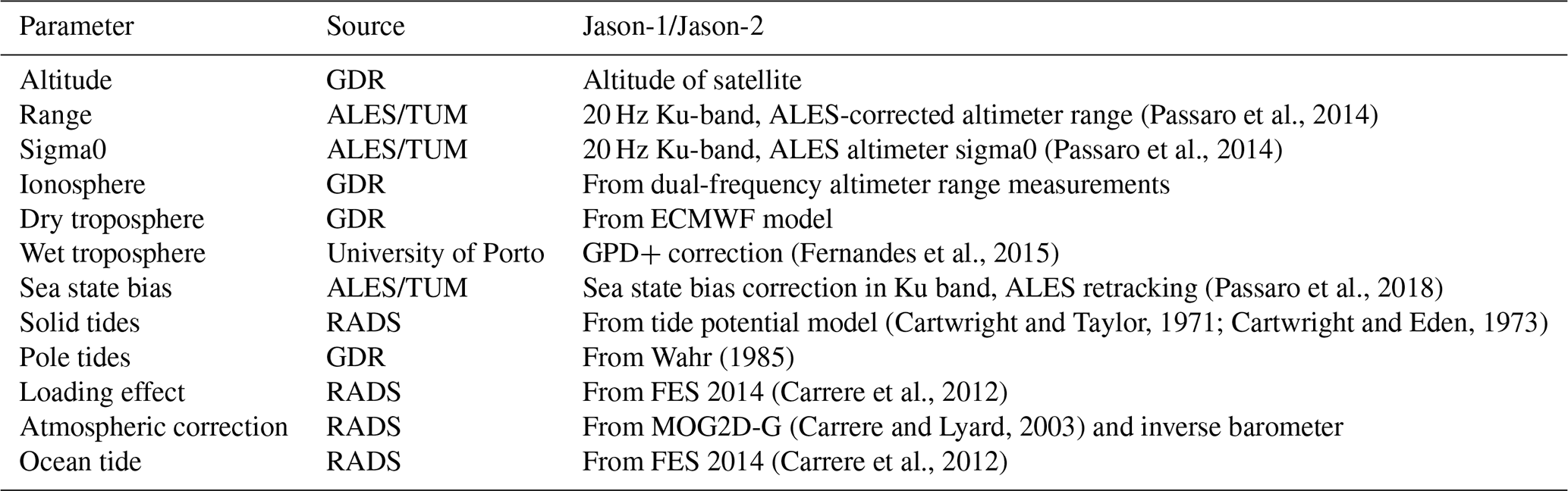
The new X-TRACK/ALES processing system first downloads from the altimetry database hosted by the French National Observations Service for altimetry called CTOH (http://ctoh.legos.obs-mip.fr/, last access: 17 September 2020) all parameters needed to compute the sea level anomaly (orbit solution, altimeter range, and instrumental, environmental, and geophysical corrections). These parameters come from the Geophysical Data Records (GDRs) data sets distributed by the space agencies for the different altimetry missions. ALES range and ssb products come from the Technical University of Munich (TUM). Additional geophysical corrections are provided by the RADS altimeter database (http://rads.tudelft.nl/rads/rads.shtml, last access: 17 September 2020) and the University of Porto (for the GPD+ wet tropospheric correction; Fernandes et al., 2015). Concerning the geophysical corrections, we used the standards defined in the ESA CCI sea level project (http://www.esa-sealevel-cci.org/, last access: 17 September 2020). These are summarized in Table 1.
Table 1List of altimetry parameters and geophysical corrections used in the computation of the coastal sea level products.
A dedicated editing strategy was further applied to eliminate noisy data. For each orbit cycle, the temporal behavior of each geophysical correction was analyzed along the satellite track. Abrupt changes were considered spurious and removed (Birol el al., 2017). This strategy has proved to be very efficient in recovering a significant amount of valid altimeter measurements that were otherwise flagged in the standard GDR products (Jebri et al., 2016). In a second step, all corrections were recomputed at the 20 Hz high rate using only the valid data through interpolation/extrapolation methods. The sea level data of each cycle were further projected onto fixed points along a nominal ground track and converted into SLAs by subtracting a reference mean sea surface height. At this stage of the processing, a regional data set of SLA time series with a spatiotemporal resolution of 10 d and 20 Hz (∼0.3 km) was produced for each Jason mission. To obtain a single multi-mission product, an inter-mission bias was estimated and removed. This was done at regional level by computing the mean sea level differences between the two missions over their overlapping period (calibration phase). The resulting SLAs were further averaged on a monthly basis at every 20 Hz point, and additional editing was performed to remove outliers (details in Marti et al., 2019).
In this study, we focus on the section of Jason track 85 located off the southwestern coast of Corsica island (western Mediterranean Sea) (see Fig. 1).
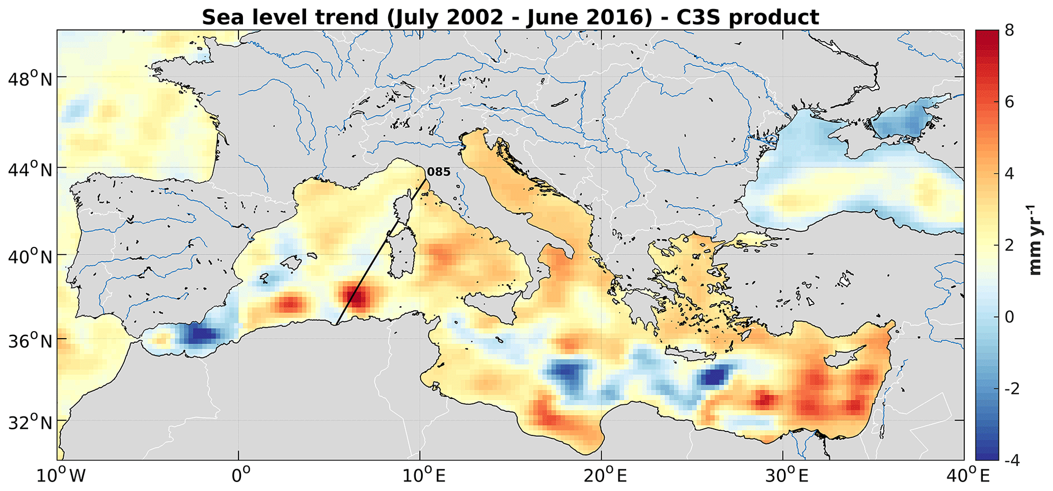
Figure 1Location of Jason track 85 crossing Corsica at the Senetosa site (straight black line). The background map shows sea level trends over 2002–2016 based on gridded altimetry data from the Copernicus Climate Change Service (C3S; https://climate.copernicus.eu/sea-level, last access: 17 September 2020).
Since 1998, a calibration site of the TOPEX/Poseidon and Jason missions has operated near the Senetosa lighthouse with support from CNES (Centre National d'Études Spatiales, France), NASA (National Aeronautics and Space Administration, USA) and the Observatoire de la Côte d'Azur (France). It is equipped with different in situ instrumentation, including weather stations, several tide gauges and a GNSS antenna. Since 1998, this calibration site has been widely used to validate the altimetry-based sea surface height data (Bonnefond et al., 2003a, b, 2010, 2011). Figure 2 is a Google Earth image of the coast showing the geographical configuration of the Senetosa calibration site with the location of the tide gauges, the GNSS antenna and the Jason track. Three tide gauges were operating during our study period (M3, M4 and M5). M4 and M5, a few tens of centimeters apart, are located on the western part of the coastline sheltered from northwesterly wind forcing. M3, 1.7 km east of M4 and M5, is more exposed to open sea conditions from the west.
Vertical land motion time series are available from the GNSS reference receiver located close to the lighthouse (G0 reference marker in Fig. 2). The tide gauges have been regularly leveled relative to the G0 reference marker with no relative motion detected so far at the millimeter level over 10 years. Trends in sea level and vertical land motions derived from these instruments at Senetosa are discussed in Sect. 5.
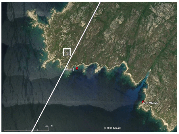
Figure 2© Google Earth image of the Senetosa calibration site. The two tide gauge sites (referred as M4/M5 and M3) are shown by the red dots. The G0 reference marker (G0) is indicated by a white square and the Jason ground track by the straight white line.
4.1 Coastal sea level trends derived from altimetry data
Following the data processing described above, we focus on monthly SLA time series sampled at 20 Hz (∼350 m in the along-track direction) from 15 km offshore to the coastline. Examples of along-track SLA time series at coastal points, located at 1, 1.6, 2.2, 5 and 15 km from the coast, are shown in Fig. 3.
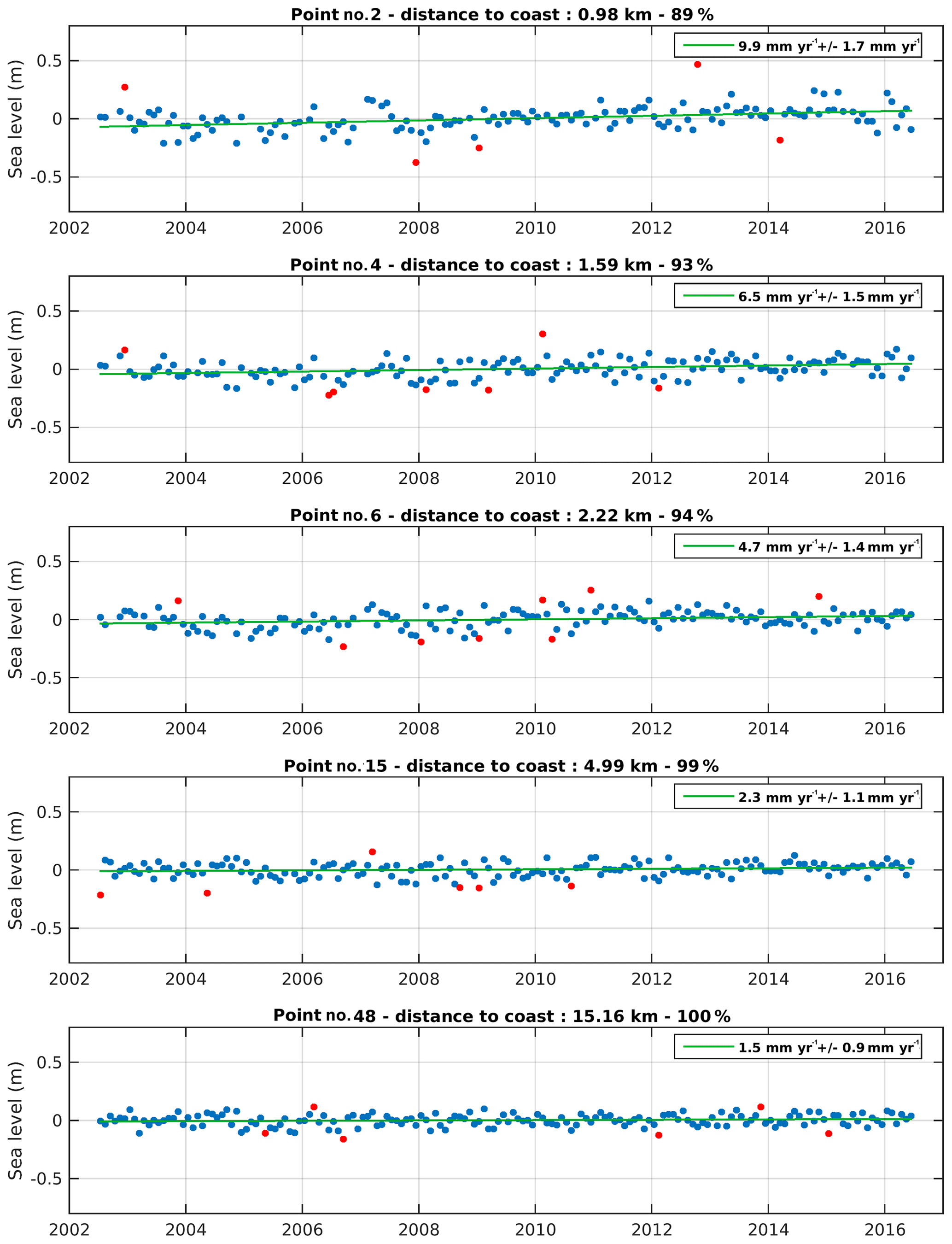
Figure 3Examples of sea level anomaly time series for 20 Hz points located at different distances from the coast. The distance to the coast, percentage of valid data and sea level trends are indicated on each plot. The green curve is the regression line adjusted to the data. The red points on the time series correspond to outliers detected using a simple 2σ filter (sigma corresponding to the SLA standard deviation). These are not considered to compute the regression line.
For each 20 Hz point, we have then computed the regression line of the resulting SLA time series and the associated standard deviation (1σ) based on the least squares fit to estimate sea level trends over the study time span. Corresponding along-track sea level trends against the distance to the coast (from 15 km offshore) are shown in Fig. 4.
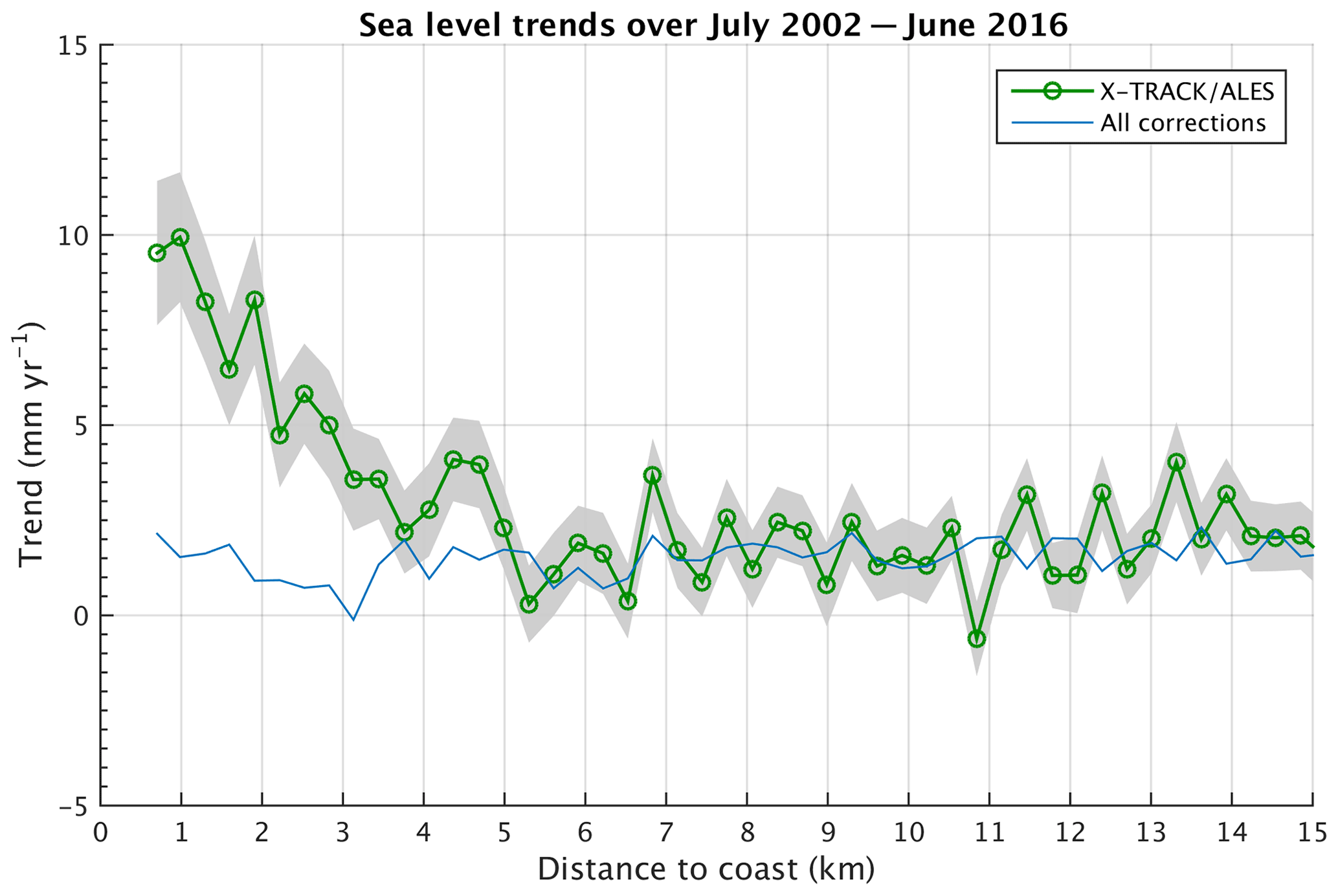
Figure 4Altimetry-based sea level trends over July 2002–June 2016 around Senetosa against the distance to the coast. Shaded area corresponds to the trend uncertainty range. The light blue curve is the sum of trends in individual corrections.
As shown in Fig. 4, beyond ∼5 km from the coast towards the open sea, the trend over 2002–2016 is relatively stable and on average on the order of 2–3 mm yr−1. High frequency oscillations around this value are observed between adjacent points, but these are likely due to noise, and we note they are of the same order of magnitude or only slightly larger than the standard deviation of trend estimates at each point (of ∼1.5 mm yr−1).
As also shown in Fig. 4, we note an almost continuous increase in the trend in the last ∼4–5 km to the coast. The corresponding trend uncertainties (standard deviation) are not significantly larger than offshore (<2 mm yr−1).
4.2 Robustness of the computed coastal trends
In coastal areas, the precision of sea surface height from altimetry is limited by inaccuracies in some of the applied geophysical corrections (including sea state bias, wet tropospheric correction, dynamical atmospheric correction and ocean tides) and from the distorted shape of the radar waveforms as the satellite approaches land (Vignudelli et al., 2011; Cipollini et al., 2018).
The corresponding altimetry measurements are often discarded by the processing chains or flagged in the data sets as potentially erroneous, leading to low confidence sea level trend estimates near the coastline. These estimates can also be impacted by the lower percentage of valid data in the coastal zone, as well as by the uncertainty in the bias estimate between the two successive missions Jason-1 and Jason-2. In order to check whether the sea level trend increase close to the coast reported in Sect. 4.1 is associated with one of these factors, each of them is independently examined.
4.2.1 Coastal errors in the geophysical corrections
We first computed and plotted the geophysical correction trends against the distance to the coast for the sea state bias, wet atmospheric correction, atmospheric loading (called DAC, dynamic atmospheric correction), and ocean and loading tide correction (Fig. 5).
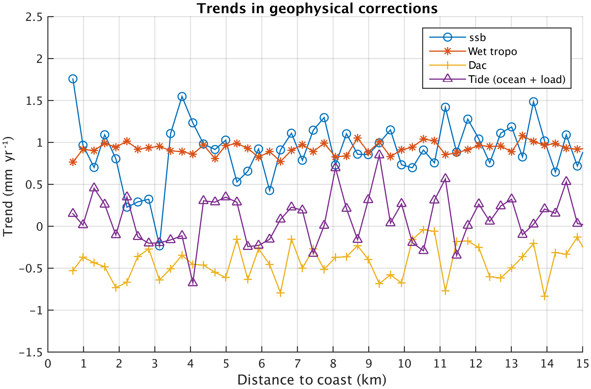
Figure 5Trends in the geophysical corrections (ssb, wet tropospheric correction, dynamic atmospheric correction, DAC, and ocean tide plus ocean loading tide) as a function of distance to the coast. Note that the vertical scale is different from Fig. 4.
Trends in the geophysical corrections are rather small, and their amplitude is in the range of ±1 mm yr−1 except for the ssb that shows a larger trend within 4 km of the coast but always less than 2 mm yr−1. It is worth mentioning that the ssb is a function of significant wave height (SWH) and backscatter coefficient sigma0 (both related to wind speed). In the ALES retracking, the ssb is recomputed for each 20 Hz point. So a trend in ssb may be due either to a different behavior of the SWH and wind speed at the coast or to changes in backscatter properties.
The sum of these geophysical correction trends is plotted in Fig. 4 (blue line). Even if the geophysical corrections, and especially the ssb, are more uncertain close to the coast, Fig. 4 suggests that the continuous increase in the sea level trends observed in the last ∼4 km to the coast may not be due to trends in the geophysical corrections. It remains that the empirical formulation used for the ssb correction may not be valid close to the coast where waves could have a different behavior compared to the open sea. This will be discussed in Sect. 6.1.
4.2.2 Coastal changes in the percentage of valid data
We next examined the possible impact on the trend estimation of the decrease in valid data in the last 3–4 km to the coast. The original percentage of valid data at each 20 Hz point decreases with distance from the coast, as shown in Fig. 6. We resampled the along-track sea level records, keeping only the 80 % of data common to all along-track positions at a given time.
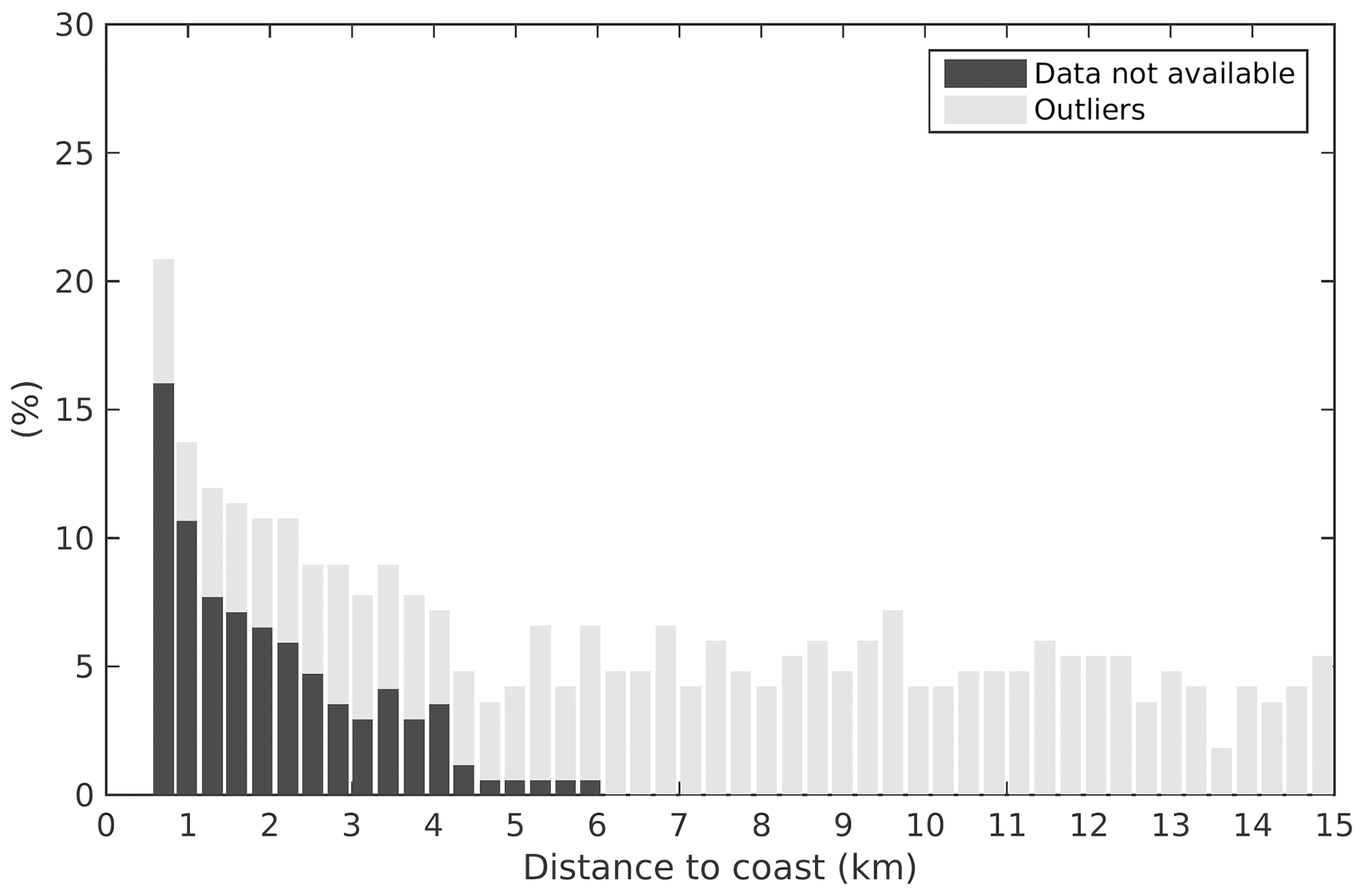
The along-track sea level trends were recomputed with the new sampling (80 % of the original data kept) (Fig. 7). For comparison, in Fig. 7 we superimpose the trends computed with the original sampling. Trends compare well in both cases. Even if the trend values are slightly lower in the band of 0–5 km, keeping only 80 % of the valid data does not significantly change the coastal trend behavior. We conclude that the lower amount of valid near-shore altimetry data does not explain the trend increase observed as the distance to the coast decreases.
4.2.3 Effect of inter-mission bias estimation
As discussed in detail in Marti et al. (2019), in the X-TRACK/ALES sea level product, the bias applied to combine the Jason-1 and Jason-2 data in a single sea level time series was estimated at a regional scale. In the case of our study region, it was estimated over the whole Mediterranean Sea. In order to investigate a possible impact of this approach on the sea level trend estimates, we tested other bias calculation methods. We first recomputed the inter-mission bias along Jason track 85 (using only measurements of this particular track). In another test, the bias was computed from data included in a 1∘×1∘ box around the Senetosa site. The sea level trends derived from the corresponding Jason-1 and Jason-2 time series are shown in Fig. 8a for these two cases, which are superimposed on the regional bias case shown in Sect. 4.1. Here again we can see that there is almost no difference between the results of the three approaches, indicating that inadequate inter-mission bias estimate does not explain the coastal trend increase. To complete these tests, we also recomputed SLA trends as a function of distance to the coast using as reference a local geoid computed for altimetry mission calibration purposes (P. Bonnefond, personal communication, 2019). Figure 8b shows the geoid profile as a function of latitude, together with the along-track mean sea surface height computed with the altimetry data. Both references compare well. Thus, as expected, exactly the same trend increase behavior against the distance to the coast is observed when the reference geoid is used (figure not shown as it is similar to Fig. 4). We conclude that the reference has no impact on the computed trends.
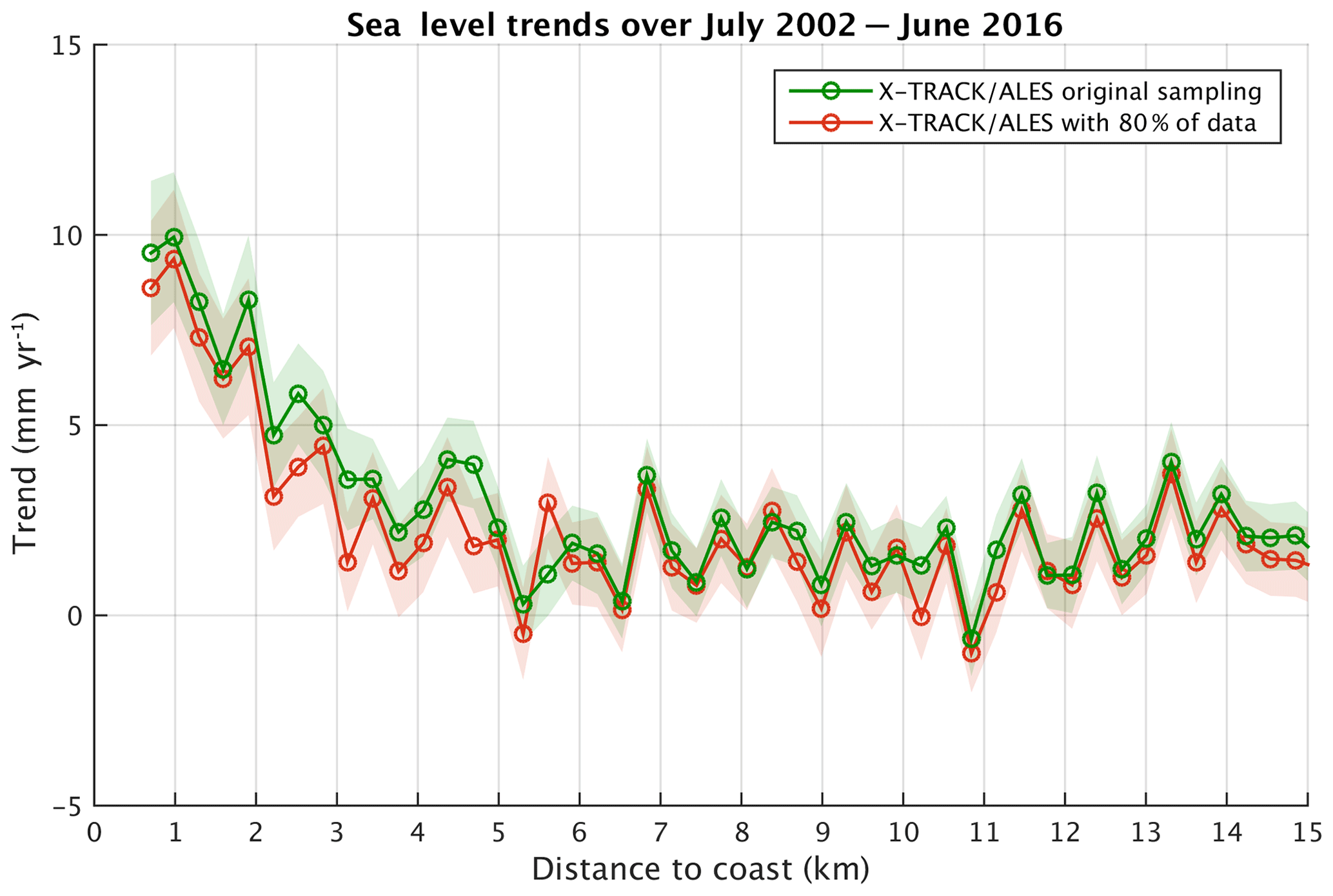
Figure 7Sea level trends against the distance to the coast with the original data set (green curve) and new sampling (80 % of original data kept; red curve).
4.2.4 Coastal altimetry waveforms and range values near Senetosa
In another series of tests, we examined the shape of the radar waveforms at 20 Hz points as a function of distance to the coast, considering a few Jason cycles taken at random. An example is shown in Fig. 9 for a point located between the coast and 2 km offshore. Figure 9 shows that at the Senetosa site, the leading edge of the coastal radar echo is generally well defined, suggesting that a robust determination of the range is possible very close to the coast.
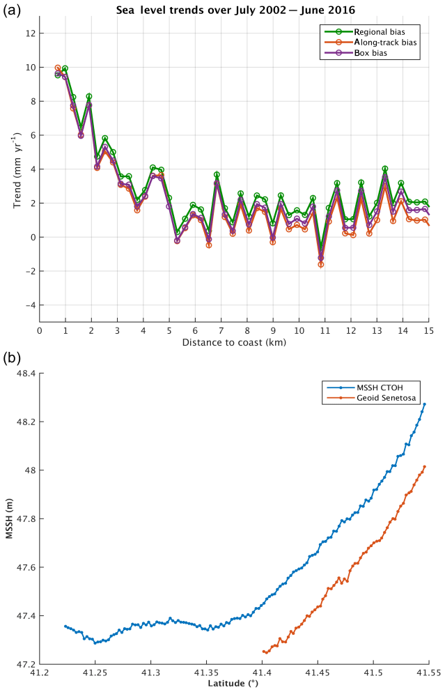
Figure 8(a) Sea level trends against the distance to the coast for three different inter-mission bias estimates. (b) Geoid and altimetry-based along-track mean sea surface profiles against latitude. MSSH CTOH stands for mean sea surface height determined by CTOH.
To investigate this further, we tried to assess the reliability of successive 20 Hz ALES-based range data very close to the coast. The waveform amplitude represents the radar power as a function of time. For Jason-2, time is discretized into 104 successive “gates”. Knowledge of the orbit and radar footprint allows us by simple geometric analysis to associate a point on the ground (pixel) to a given gate. A numerical simulation has been performed for that purpose (assuming flat land) in order to produce range maps for Jason track 85 with the goal of precisely locating the point on the ground corresponding to the measured waveform. This is illustrated in Fig. 10a and b, which show the geographical configuration and associated radar waveforms for two range measurements located at 0.53 and 1.4 km distance from the coast. The range measurement deduced from the waveform corresponds to the center of the circle representing the radar footprint on the range map.
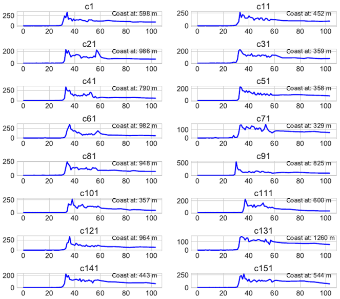
Figure 9Observed radar waveforms at points close to the coast for a series of Jason cycles (the number on each plot refers to cycle number).
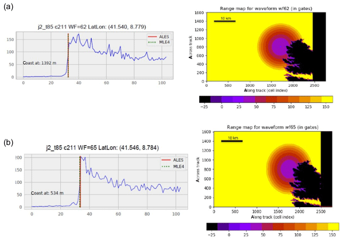
Figure 10(a) Radar waveform against gate number (left) and configuration of the radar footprint on the ground (right) at 1.4 km from the coast. (b) Same as (a) but at 0.5 km from the coast.
Although these simulations represent an ideal case of smooth sea state and flat land, Fig. 10a and b show that even at the closest point to the coast (0.5 km), the leading edge of the return waveform still corresponds to a reflection of the radar signal on water. This suggests that it is theoretically possible to retrieve valid sea level information up to 0.5 km from the coast. One may argue that because the land at Senetosa has some elevation, the real radar echo is partly contaminated by land reflection at distances larger than the theoretical footprint even if there is no wave. However, considering that the real waveform has a leading edge and that the retracker is able to follow it, we conclude that the trends reported on successive 20 Hz points are not spurious. Besides, if the retracker was corrupted by inhomogeneous backscatter properties within the satellite footprint, these should be random (e.g., Passaro et al., 2014). Finally, 20 Hz waveforms being independent samples, if the retracker is wrong and produces spurious trends, the latter also would be random. Thus, we should not see a continuous trend increase over several consecutive points.
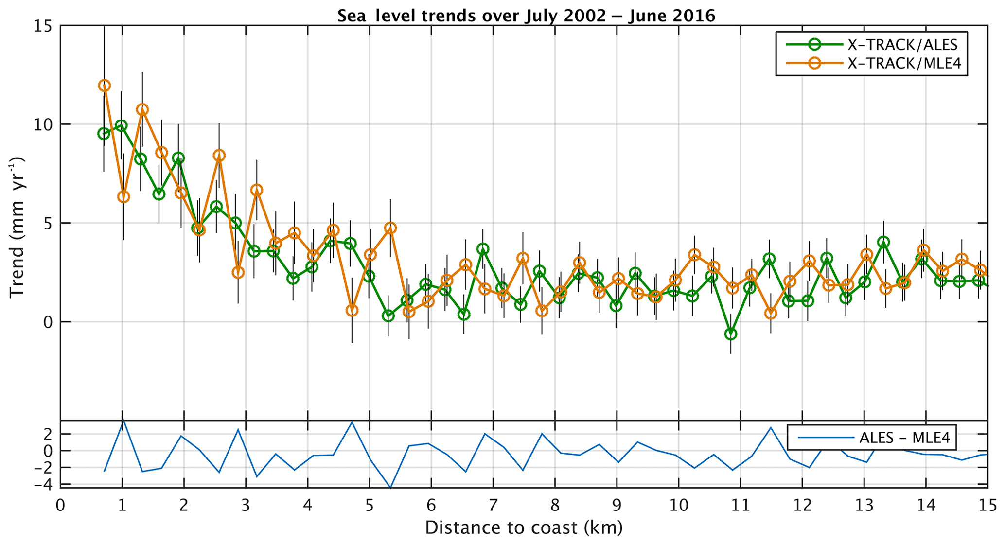
Figure 11Sea level trends against the distance to the coast for MLE4-based (orange dots) and ALES-based (green dots) SLA data. Vertical bars correspond to trend errors (1σ). The light blue curve at the bottom of the panel represents the difference between ALES-based and MLE4-based trends.
4.2.5 Comparison between ALES and MLE4 retrackers
Finally, we performed the same analysis (computation of sea level trends as a function of distance to the coast) using SLA data computed with the classical MLE4 (maximum likelihood estimator) retracker (used for the standard Geophysical Data Records production; https://www.aviso.altimetry.fr/fileadmin/documents/data/tools/hdbk_tp_gdrm.pdf, last access: 17 September 2020). MLE4-based trends over the 14-year time span are shown in Fig. 11, in which the ALES-based trends are superimposed for comparison. We note that MLE4 gives noisier results than ALES, especially at distances less than ∼5 km to the coast, but the increase in trends in the last ∼4–5 km to the coast is still clearly visible. This clearly means that the trend increase is not an artifact due to the use of the ALES retracker.
To summarize, from all the tests presented above, we can conclude that the increase in altimetry sea level trend observed in the last 4–5 km from the coast is not correlated with errors in the geophysical corrections and is not explained by the loss of valid data nor the presence of spurious waveforms or by the inter-mission bias. Furthermore, the calculated trends are robust to changes in the retracker since instead of using ALES, we also used the standard high-frequency MLE4 retracker. The corresponding time series still show the same trend behavior (although with noisier results).
It is very classical to validate altimetry-based sea level data by comparing them with tide gauge records. The availability of tide gauge records at the Senetosa site is a good opportunity to do so. Tide gauge data have been provided by the Observatoire de la Côte d'Azur (Géoazur Laboratory) and can be downloaded from http://www.aviso.altimetry.fr/en/data/calval/in-situ/absolute-calibration/download-tide-gauge-data.html (last access: 17 September 2020). The high-frequency tidal signal and the atmospheric forcing effect have been removed (using the same DAC correction as for the altimetry data). The time series have been further smoothed on a monthly basis. The corresponding tide gauge time series over 2002–2016, for the M3, M4 and M5 tide gauges, are shown in Fig. 12a and b with and without the seasonal cycles.
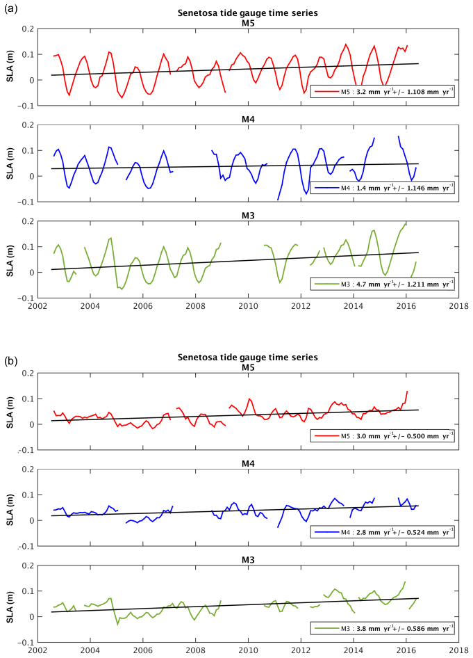
Figure 12Sea level time series based on in situ tide gauge measurements at the M3, M4 and M5 sites over 2002–2016 (a) with the seasonal cycle and (b) without the seasonal cycle.
From these time series, we computed linear trends over the same period as for the altimetry data. These are gathered in Table 2 for the two cases (with and without the seasonal cycle). In Bonnefond et al. (2019), it was shown that when making differences between tide gauge sea level measurements, there has been no systematic trend between the tide gauge time series since 2001 (below 0.1 mm yr−1), well within the trend uncertainties. The GNSS-based vertical land motion (VLM) at Senetosa (estimated in Bonnefond et al., 2019) is also shown. VLM is small at Senetosa at less than 0.3 mm yr−1.
Table 2Relative sea level trends (mm yr−1) recorded by the M3, M4 and M5 tide gauges (estimated with and without the seasonal cycles), as well as the GNSS-based vertical land motion (mm yr−1) at the Senetosa site.
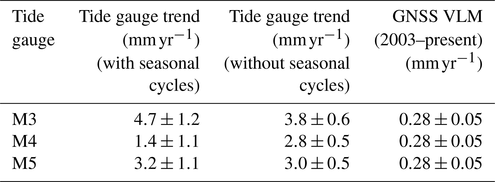
The M4 time series displays several gaps over the study period. In addition, the record (seasonal cycle not removed; Fig. 12a) shows a large positive anomaly in 2015, which was not seen by M3 or M5. M3 also has a large gap in 2009/2010, as well as other gaps in 2012 and at the end of the record. A suspect drop is also visible in 2005 in Fig. 12b (seasonal cycle removed). Thus, the M5 record seems the most reliable even if the trends from M3 and M4 are close to M5 (see Table 2). The computed (relative) sea level trend (uncorrected for the VLM) is on the order of 2.8–3.8 mm yr−1 over the study period (seasonal cycle removed). If the GNSS VLM trend is accounted for, this range becomes 3.1–4.1 mm yr−1. This value is significantly less than the altimetry-based sea level trends reported here in the last 4–5 km to the coast. On the other hand, the tide gauge trend agree well with the altimetry-based trends reported at distances greater than 4 km from the coast. While the reported altimetry-based sea level trend increase may disqualify our retracked sea level data in the vicinity of the coast, in the next section we discuss the possibility that some coastal processes affect sea level in a band a few kilometers from the coast while being attenuated very close to the shore where the tide gauges (in particular M5) are located.
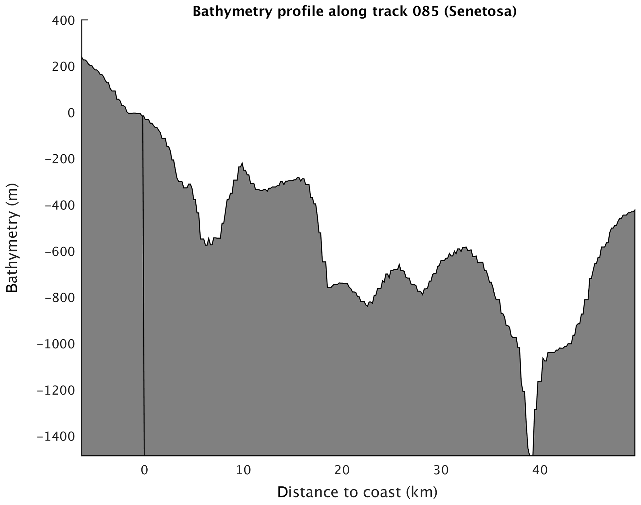
Figure 13Bathymetric profile (meters) along Jason track 85 from 45 km offshore to the coast.
Compared to deep-ocean sea level, sea level close to the coast can be impacted by various small-scale processes resulting from the morphology of the coastline, the depth of the continental shelf, the presence of a river estuary, etc. (Woodworth et al., 2019). Thus, coastal sea level may significantly differ from open-ocean sea level over a large range of temporal scales. In terms of trends, the open-ocean sea level essentially results from processes affecting the global mean sea level (mean ocean thermal expansion, land ice melt and land water storage changes) (e.g., WCRP, 2018) and the superimposed regional variability (regional changes in ocean thermal expansion, atmospheric loading and fingerprints due to the solid Earth response to changing ice mass loads; Stammer et al., 2013). At the coast, in addition to these two contributions, local variations in other processes may cause additional small-scale sea level changes at interannual to decadal timescales, such as trapped Kelvin waves, upwelling/downwelling effects, eddies, wind-generated waves and swells, shelf currents, and water density changes related to river runoff in estuaries (see Woodworth et al., 2019, for a detailed discussion on forcing factors affecting sea level changes at the coast). Note that we do not discuss vertical land motion here since our objective is to understand the observed change in “geocentric” sea level as measured by satellite altimetry.
In the case of Senetosa, river runoff and trapped Kelvin waves are not supposed to affect coastal sea level. Could other processes like trends in wind-generated waves and coastal currents explain the slow increase in sea level trend towards the coast? These are discussed below.
6.1 Effect of waves on SLA and ssb
We first discuss the effect of waves. The contribution of wind-generated waves to coastal sea level changes has been investigated in a number of recent studies (e.g., Melet et al., 2018; Dodet et al., 2019). As thoroughly discussed in Dodet et al. (2019), wind-generated waves have the capability to significantly change sea level variations at the coast even on the timescales of interest here. The shoaling and breaking of waves on the shallow water shelves raise the mean water level in the so-called near-shore and surf zones (last ∼1 km to the coast), a process called wave setup. Wave setup is proportional to offshore significant wave height, and if the latter displays a temporal trend due to a trend in wind forcing, it may cause a sea level trend in the coastal zone.
The relationship between offshore wave height and wave setup is known empirically only (Dodet et al., 2019). To the first order, wave setup is related to offshore SWH, wave period and beach slope. The bathymetric profile along Jason track 85 (from 45 km offshore to the coast) is shown in Fig. 13. We note an abrupt increase of more than 500 m in the last 5 km to the coast, corresponding to a slope of 0.1.
If the bathymetric slope near Senetosa is known, it is not the case for other parameters involved in the relationship between SWH and wave setup. This is the case in particular for beach soil characteristics, sediment size, etc. A large variety of formulations have been proposed for this relationship based on in situ observations collected at different coastal sites (e.g., Dodet et al., 2019). However, these are not necessarily applicable to our study case as some local beach parameters are not known. It is generally assumed that wave setup does not exceed 20 % of SWH. Thus, as a preliminary approach, we analyzed offshore SWH data only in order to highlight their temporal variability over our study time span.
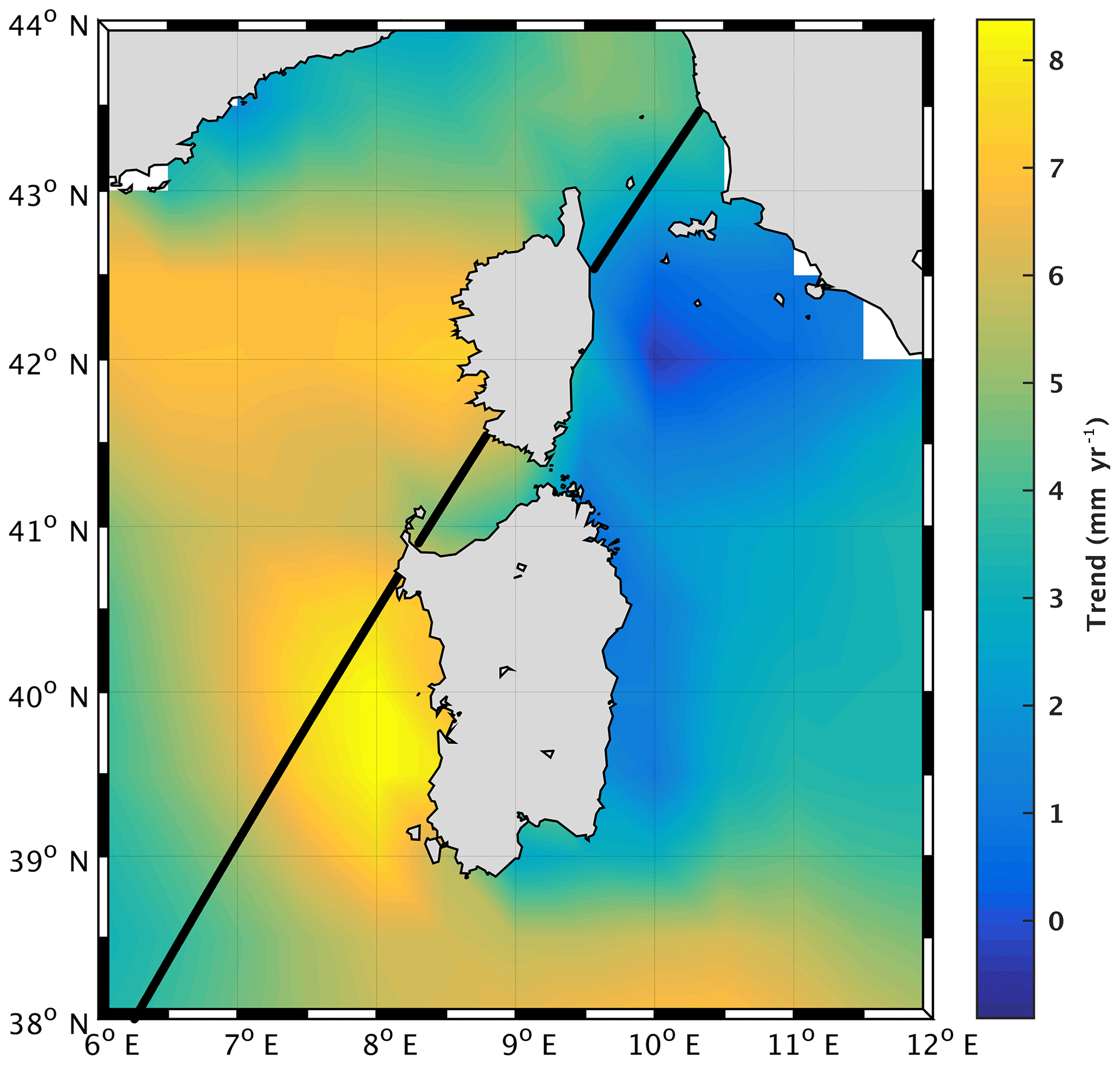
Figure 14Wave height trends (in mm yr−1) over 2002–2016 in the western Mediterranean Sea (data from ERA5 reanalysis).
For that purpose, we considered wave field data from the ERA5 reanalysis (https://www.ecmwf.int/en/forecasts/datasets/reanalysis-datasets/era5, last access: 17 September 2020; https://apps.ecmwf.int/data-catalogues/era5/?class=ea, last access: 17 September 2020). The ERA5 reanalysis provides gridded SWH time series at monthly intervals from 1979 to the present, thus covering our study period. The grid size resolution is 0.5∘. Using this data set, we computed 2-D SWH trends over 2002–2016, as shown in Fig. 14. We note high positive wave height trends west of Corsica and Sardinia over this period. Along Jason track 85 in the vicinity of Senetosa, the trend is on the order of 5 mm yr−1. Note that we also computed the wind trend using the same ERA5 reanalysis gridded data over the same period (2002–2016). The map (not shown) displays positive trends in wind south of Corsica, although with a smaller amplitude than along the western coast of Sardinia, like the wave height map shown in Fig. 14.
From the above discussion, we deduce that wave setup would not contribute by more that 1 mm yr−1 to the coastal sea level trend. Noting in addition that wave setup would affect sea level in close vicinity to the coast only (i.e., not over 4–5 km distance; X. Bertin, and J. Wolf, personal communications, 2019), it is very unlikely that wave setup explains the reported coastal sea level trend.
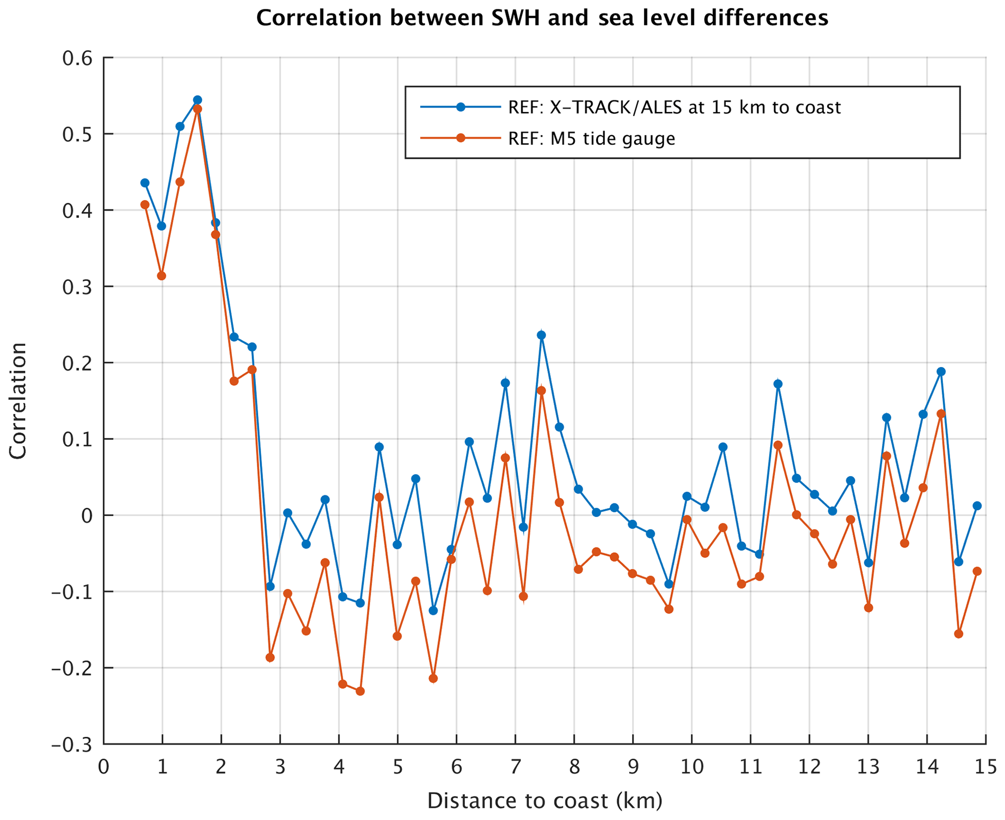
Figure 15Correlation between the wave height (SWH) time series (from ERA5 grid mesh close to Senetosa) and altimetry-based sea level difference time series between every 20 Hz point and a reference point. The blue curve corresponds to a reference time series for a point located 15 km from the coast. In the case of the red curve, the reference time series is the M5 tide gauge record.
We further investigated the effect of waves on the ssb correction, hence on SLAs. For that purpose, we computed the correlation between wave height time series and difference in sea level between each 20 Hz altimetry point and a reference altimetry point located in the open ocean (chosen here at 15 km from the coast). We consider differences in sea level anomalies in order to remove the common ocean signal affecting sea level close to the coast and offshore, e.g., the global mean sea level rise and its superimposed regional variability. By computing the sea level differences between 15 km offshore and the coast, the latter large-scale sea level components are removed, leaving only small-scale signals occurring very close to the coast. Data from the ERA5 grid closest to Senetosa were used (the center of the considered grid point is located 41.5∘ N, 8.5∘ E at 24 km from the first valid point on the Jason track and 25 km from Senetosa). The correlation values are shown in Fig. 15 against the distance to the coast. From a distance of ∼3 km from the coast towards the deep sea, the correlation between wave height and sea level difference is insignificant, while it clearly increases from ∼3 km to the coast. This suggests that there is a link between the variations in waves and SLA variations in the 0–3 km domain close to land.
We performed the same analysis but now using the M5 tide gauge record as reference (the M3 tide gauge record had too many data gaps). This is also shown in Fig. 15. Surprisingly, we find exactly the same behavior of the correlation coefficient, i.e., no correlation offshore (points located at a distance of more than 3 km from the coast) and an increase in correlation in the last 3 km to the coast. This suggests that waves may affect SLA only in the domain 0–3 km from the coast but that at the tide gauge site, waves have no influence. Obviously, this could be via the ssb correction applied to SLA data.
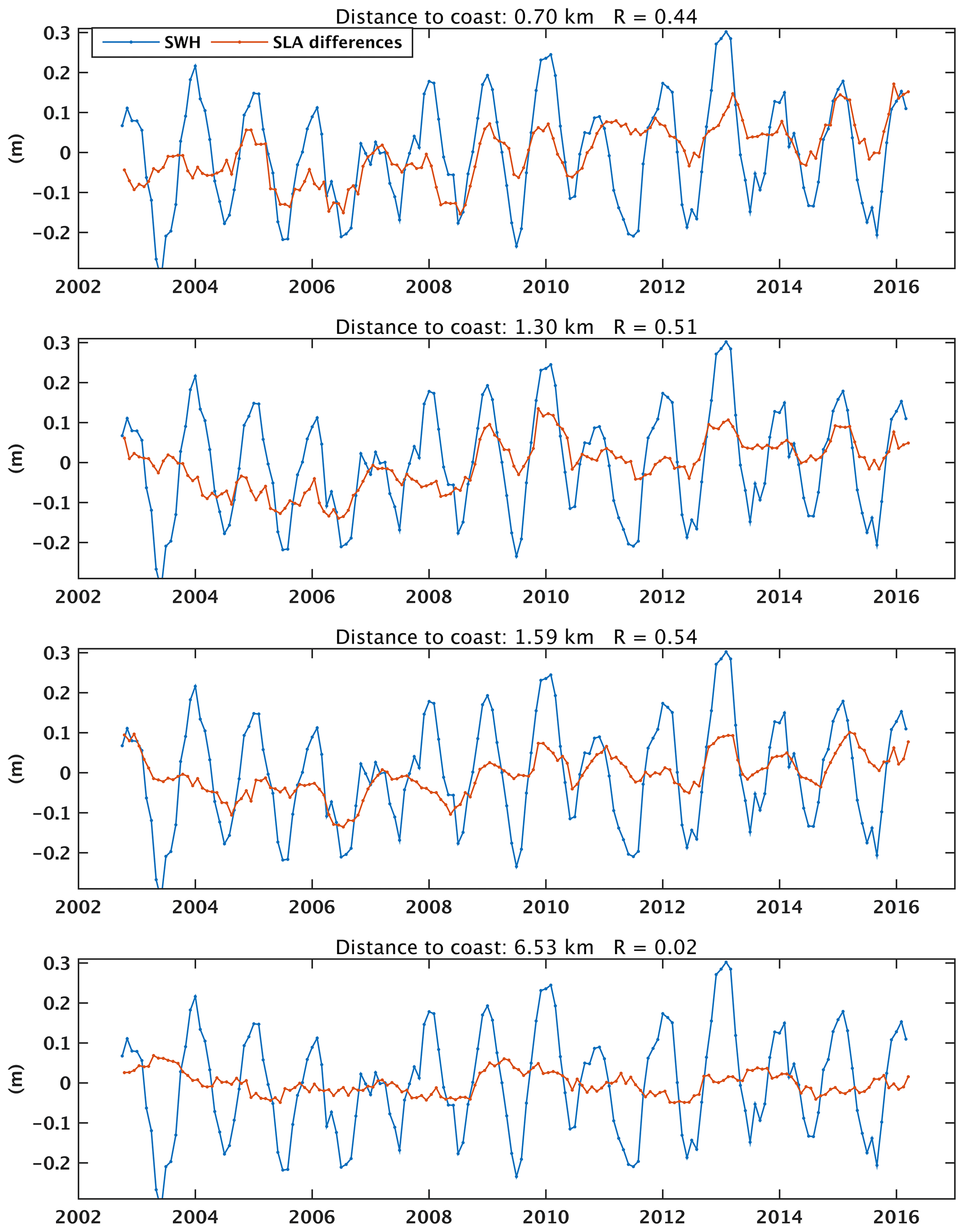
Figure 16Time series of ERA5-based wave height time series (blue curve) and of altimetry-based SLA differences (orange curve) between 20 Hz points at different distances from the coast (indicated on each plot) and a reference point (located at 15 km).
It has been demonstrated that applying the ssb correction to altimetry data, in particular to high-frequency data as in this study, reduces the correlation between SWH and range (and, consequently, SLA) (Passaro et al., 2018). The ssb correction is mainly a function of SWH; it removes from the range estimation an effect that is directly proportional to the wave height. This means that if this ssb correction is not applied, it has to be expected that the SLA record will be correlated with the SWH record. To illustrate this somewhat differently, Fig. 16 shows wave height time series superimposed to altimetry-based differences in SLA time series (reference point at 15 km, as in Fig. 15) for a few points located in the 0–3 km domain close to the coast and an additional point located farther from the coast. Here again, data from the ERA5 grid closest to Senetosa have been considered for the calculation. The correlation between SWH and difference SLA time series is indicated on each plot. We clearly see that it is significant only for points close to the coast. Distant offshore points do not show such a correlation. Although the correlation is dominated by the seasonal signal, Fig. 16 shows that the two time series are also correlated at interannual timescales.
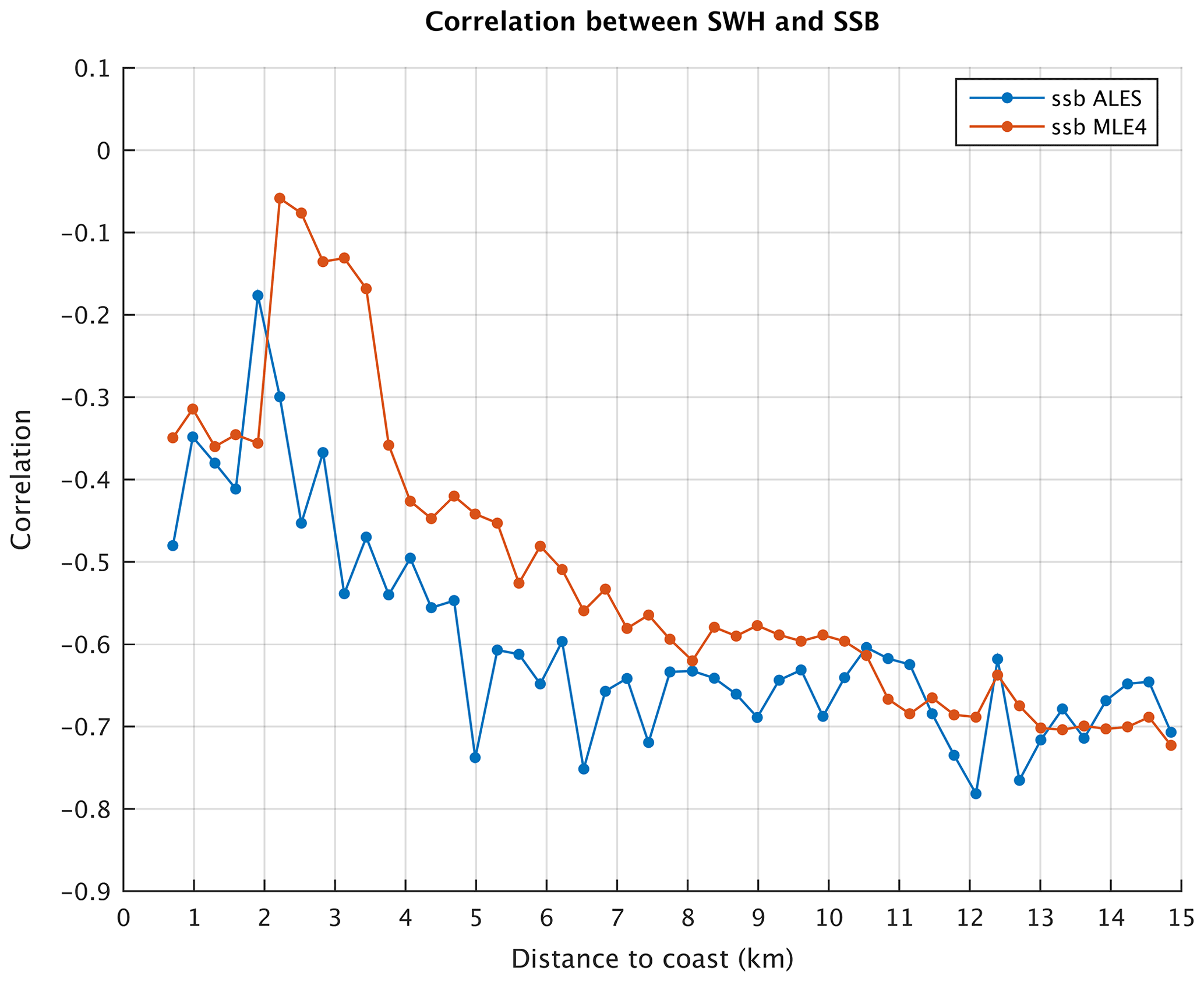
Figure 17Correlation between significant wave height (SWH) time series and ssb time series between every 20 Hz point and a reference point.
We argue that when the range close to the coast is not being properly corrected for the ssb, this results in a lesser correlation between ssb and SWH. To verify this, we repeated this correlation analysis but now using the ssb correction (from both the ALES and MLE4 retrackings) instead of the SLA differences. As expected, ssb is correlated with SWH away from the coast (−0.75 and −0.56 at 6.5 km from the coast for MLE4 and ALES, respectively), but the correlation decreases in the last few kilometers to the coast (amounting to −0.35 and −0.48 at 0.7 km from the coast for MLE4 and ALES, respectively). This suggests that the relationship used to express the link between ssb and SWH is less adapted to the coastal domain than to the open sea either because of a change of wave properties (which makes the ssb model invalid) or because of an incorrect estimation of SWH very close to the coast. This is also illustrated in Fig. 17 which shows the correlation between ssb and SWH against the distance to the coast (for both ALES ssb and MLE4 ssb). Between 1 and 4 km, the correlation between SWH and ssb decreases. It is worth noting, however, that the correlation remains higher for ALES ssb than for MLE4 ssb.
We conclude from these tests that the correlation between SLA and wave height at 20 Hz points close to the coast is very likely due to imperfect ssb correction. Thus, we can now exclude any direct effect of waves (e.g., trend in wave setup) as a candidate to explain the SLA trend increase close to the coast. Whether the reported SLA trends in the last few kilometers to the coast are due to the inadequate formulation of the relationship between SWH and ssb as the satellite approaches the coast remains so far an open question. While we cannot exclude that the ssb correction is imperfect close to the coast, it seems unlikely that it would produce such large trends as those observed in the SLAs.
6.2 Effect of coastal currents and comparison with an ocean model
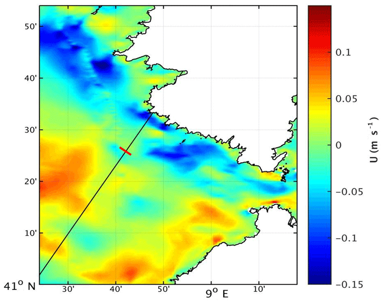
Figure 18Barotropic current (zonal component U) for January 2014 based on the MARS3D hydrographic model. The blue color means westward current. The Jason track (black line) crosses this current at 4 km from the coast. The red bar crossing the Jason track indicates the 15 km distance from the coast.
In this section we briefly address the effect of coastal currents on the SLAs. There are only few published studies on the circulation in the Senetosa region (e.g., Bruschi et al., 1981; Manzella et al., 1985; Cucco et al., 2012; Gerigny et al., 2015; Sciascia et al., 2019). These indicate that the dominant characteristics of the circulation in the Corsica channel (Straight of Bonifacio) are a flow predominantly directed northward from the Tyrrhenian Sea to the Ligurian Sea and that the water motion is mainly wind-driven. The study by Gerigny et al. (2015), based on in situ measurements collected during a cruise in 2012 and on the use of a high-resolution regional hydrodynamic model (MARS3D), shows that the circulation is mostly wind-driven, forced by westerly winds half of the year and strong easterly winds in winter generating strong local currents and mesoscale structures in the western part of the channel. We have downloaded the current data generated by the MARS3D model, a coastal hydrodynamical model developed by IFREMER (Institut Français de Recherche pour l'Exploitation de la Mer; Lazure and Dumas, 2008). There is a high-resolution (400 m) version available for the Corsica region for the years 2014 to the present (http://www.ifremer.fr/docmars/html/doc.basic.intro.html, last access: 17 September 2020). The model does not assimilate altimetry data nor any other type of data. Because this data set has only 2.5 years of overlap with our study period, we cannot compute trends. However, to gain some insight on the circulation configuration, we examined the current patterns over the year 2014. In agreement with the literature, we observed a strong zonal current during the winter months close to Senetosa. An example of the zonal component of the barotropic current south of Corsica is shown in Fig. 18 for January 2014. We note a clear westward current along the Senetosa coast starting at ∼4 km from the coast. It is also worth noting that it does not extend to the shoreline and thus may not influence tide gauge measurements.
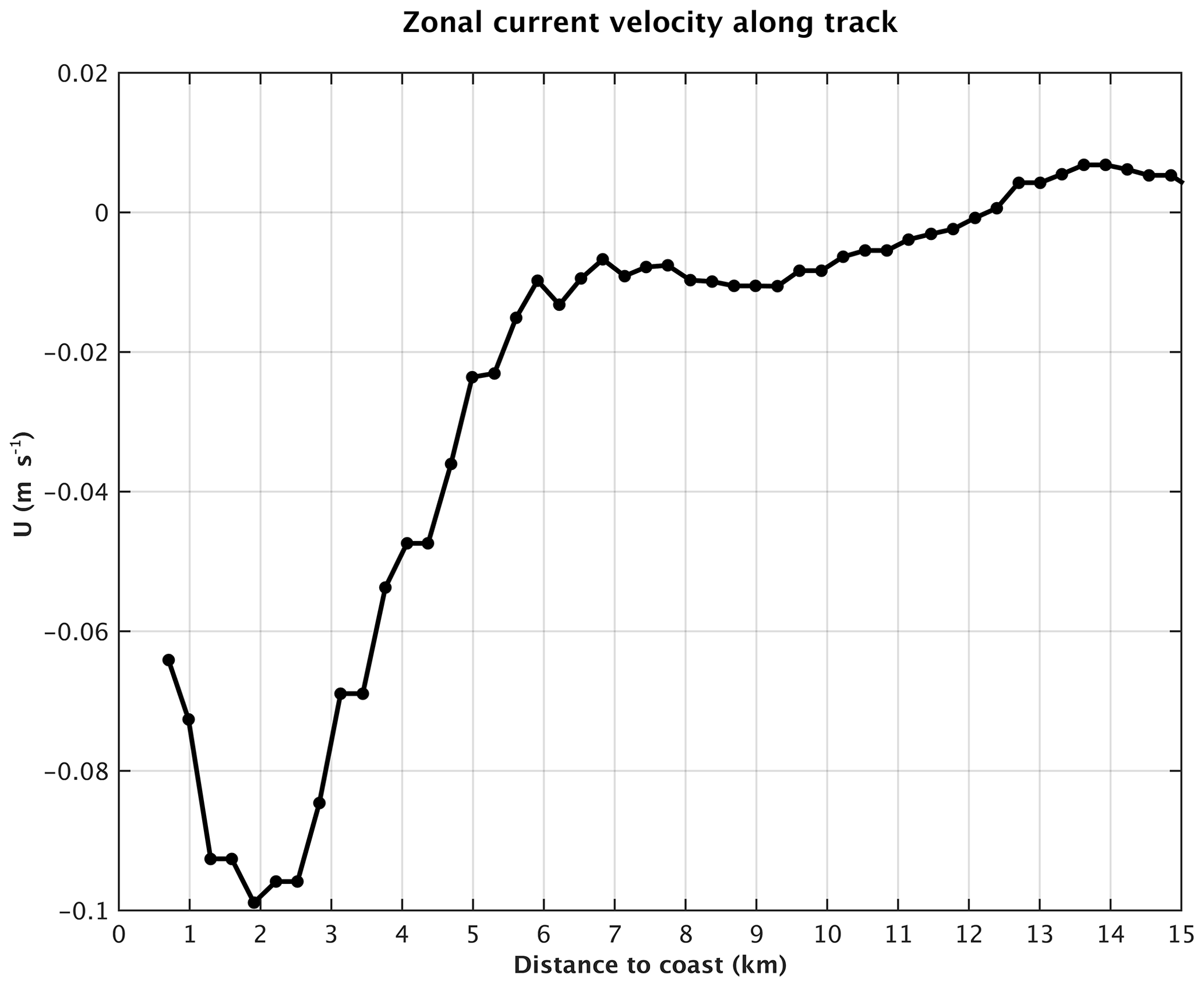
Figure 19Barotropic current (zonal component U) for January 2014 based on the MARS3D hydrographic model interpolated along the Jason track against the distance to the coast. Negative values mean westward current.
We interpolated these current data (for January 2014) along the Jason track. This is shown in Fig. 19 against the distance to the coast. The current intensity is close to 0 at distances greater than 5 km from the coast. In the last 5 km to the coast, there is a steep intensity increase exactly over the same distance range as the SLA trend increase. Since the model resolution is ∼400 m, i.e., about the same resolution as the 20 Hz along-track SLAs, we find this result highly promising.
Of course, we cannot extrapolate backward in time nor offer any solid conclusion so far, but we cannot exclude that the observed sea level trend increase is linked to an increase in intensity of this winter current during our study period. This obviously will need a much deeper investigation, at least over the time span of the availability of the model data.
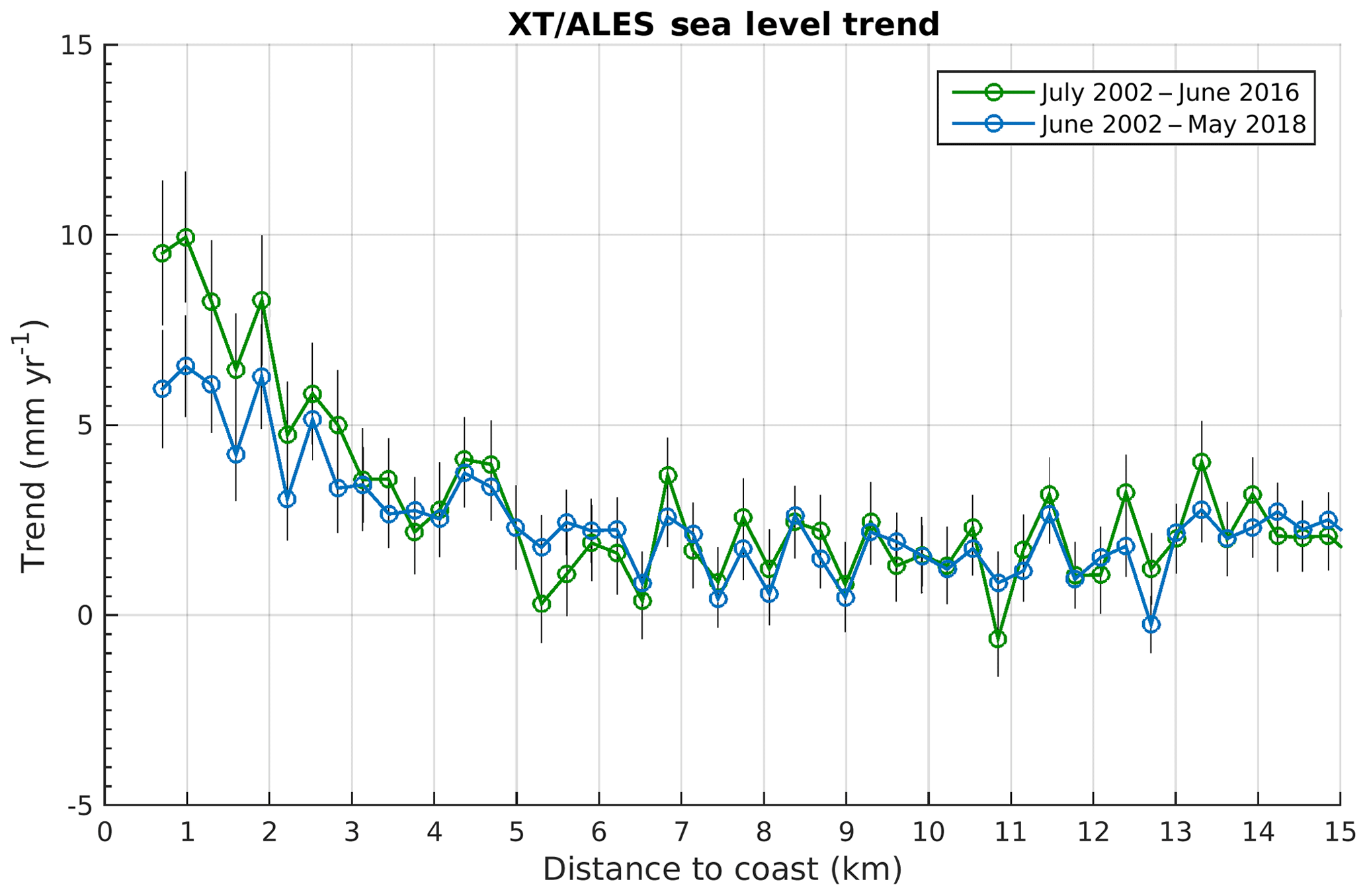
Figure 20Altimetry-based sea level trends at Senetosa over two periods: (1) July 2002–June 2016, green curve, and (2) June 2002–May 2018, blue curve. Black vertical bars correspond to trend uncertainties.
In this study, we have investigated the differences between coastal and deep-ocean sea level changes at the Senetosa site using new ALES-based retracked sea level data from the Jason-1 and Jason-2 missions. We indeed observe a slow increase in sea level trend at short (–5 km) distances from the coast compared to offshore. A series of tests shows that this behavior does not result from artifacts due to spurious trends in the geophysical corrections applied to the altimetry data, decreasing percentage of valid data, errors in the inter-mission bias, or errors in range estimates due to distorted radar waveforms.
While the paper was in review, an update of the results presented above has been recently performed extending the SLA time series with Jason-3 data up to June 2018 (coastal trends based on Jason-1, Jason-2 and Jason-3 over 2002–2018 at several hundreds of coastal sites located in six different regions worldwide are presented elsewhere; The Climate Change Initiative Coastal Sea Level Team, 2020). Although the coastal trends within 2–3 km of the coast are slightly lower than those reported above, exactly the same behavior is found, as shown in Fig. 20, which compares coastal trends over 2002–2016 and 2002–2018. Thus, the trend increase close to the coast observed at Senetosa is not due to the limited length of the time series, although its amplitude decreases as the record length increases. Similarly, the geophysical correction trends present the same behavior over both time spans. It is worth mentioning that in the extended study (2002–2018), among the 429 coastal sites studied, coastal trends do not in general differ from open-ocean trends (within ±1 mm yr−1) except at a few sites (The Climate Change Initiative Coastal Sea Level Team, 2020); Senetosa is one of them. This is why we focused on this particular site.
Among the physical mechanisms able to explain the coastal trend increase in the study region, we have first explored waves, then currents. We investigated the wave effect on sea level along the Jason track and found that wave setup has a magnitude that is too low and is localized too close to the shore to explain the observed continuous SLA trend increase in the last 4–5 km to the coast. On the other hand, the correlation reported between altimetry-based SLAs and SWH very likely results from the imperfect ssb correction applied to the data. Nevertheless, if less accurate in the coast vicinity, the ssb trend seems unable to explain the reported SLA trend increase. We next investigated the effect of coastal currents. Using the MARS3D high resolution model developed by IFREMER for coastal studies, we noted the presence of a winter current along the Senetosa coastline. The projection of this current along the Jason track (for January 2014) shows a steep increase in intensity over exactly the same distance to the coast as the SLA trend increase. This may be an indication of a current-related origin. More studies are definitely needed to confirm the results presented here. However, if further investigations confirm the effect of currents, it will be a demonstration that small-scale processes acting in the vicinity of the coast may have the capability to make coastal sea level changes drastically different from what we measure offshore with classical altimetry.
The coastal sea level data analyzed in this study are available from the Nature Scientific Data article (The Climate Change Initiative Coastal Sea Level Team, 2020; a database of coastal sea level anomalies and associated trends from Jason satellite altimetry from 2002 to 2018). The altimetry-based sea level data can be downloaded from the SEANOE repository (https://doi.org/10.17882/74354, The Climate Change Initiative Coastal Sea Level Team, 2020; a database of coastal sea level anomalies and associated trends from Jason satellite altimetry from 2002 to 2018, Nature Scientific Data, in press, 2020) (last access: 17 September 2020).
The gridded sea level data from the Copernicus Climate Change Service portal (https://climate.copernicus.eu/sea-level, Copernicus, 2016) (last access: 17 September 2020).
The ERA wave field data from the ERA5 reanalysis are available from the Copernicus Climate Change Service portal (https://cds.climate.copernicus.eu/cdsapp#!/home, ECMWF, 2017) (last access: 17 September 2020) (see also https://apps.ecmwf.int/data-catalogues/era5/?class=ea, last access: 17 September 2020).
The MARS3D model is described in Lazure and Dumas (2008) and can be downloaded from the IFREMER website (https://wwz.ifremer.fr/mars3d/) (last access: 17 September 2020).
All authors contributed in different parts of the data production and analysis. MP and CS performed the ALES retracking and performed the ssb data analysis. FL, FB and FN produced the X-TRACK/ALES coastal sea level data set. PB and OL provided the Senetosa tide gauge data. RA participated in the wave data analysis. Analyses of the sea level data and model outputs presented in this paper have been performed by YG. All authors participated in the interpretation of the results. AC wrote the first version of the paper, which was further improved by all authors. YG prepared all figures, except Figs. 9 and 10 which were prepared by FN. JFL, AC and JB are project manager, science leader and technical officer, respectively, of the CCI+ Coastal Sea Level project.
The authors declare that they have no conflict of interest.
This study is a contribution to the ESA Climate Change Initiative (CCI+) Sea Level project. Yvan Gouzenes is supported by an engineer grant in the context of this project (ESA SL_cci+ contract number 4000126561/19/I-NB). We thank a number of colleagues for very fruitful discussions on the effect of waves on tide gauges and coastal sea level, in particular (by alphabetic order) Angel Amores, Xavier Bertin, Svetlana Jevrejeva, Goneri Le Cozannet, Marta Marcos, Judy Wolf and Phil Woodworth. We also thank two anonymous reviewers and the editor for their comments and suggestions to improve the paper.
This research has been supported by the ESA.
This paper was edited by Joanne Williams and reviewed by two anonymous referees.
Birol, F. and Delebecque, C.: Using high sampling rate (10/20 Hz) altimeter data for the observation of coastal surface currents: A case study over the northwestern Mediterranean Sea, J. Mar. Syst., 129, 318–333, https://doi.org/10.1016/j.jmarsys.2013.07.009, 2014.
Birol, F., Fuller, N., Lyard, F., Cancet, M., Niño, F., Delebecque, C., Fleury, S., Toublanc, F., Melet, A., Saraceno, M., and Léger, F.: Coastal applications from nadir altimetry: example of the X-TRACK regional products, Adv. Space Res., 59, 936–953, https://doi.org/10.1016/j.asr.2016.11.005, 2017.
Bonnefond, P., Exertier, P., Laurain, O., Ménard, Y., Orsoni, A., Jan, G., and Jeansou, E.: Absolute calibration of Jason-1and TOPEX/Poseidon altimeters in Corsica, in: Special Issue on Jason-1 Calibration/Validation, Part 1, Mar. Geod., 26, 261–284, https://doi.org/10.1080/714044521, 2003a.
Bonnefond, P., Exertier, P., Laurain, O., Ménard, Y., Orsoni, A., Jeansou, E., Haines, B. J., Kubitschek, D. G., and Born, G. H.: Leveling sea surface using a GPS catamaran, in: Special Issue on Jason-1 Calibration/Validation, Part 1, Mar. Geod., 26, 319–334, https://doi.org/10.1080/714044524, 2003b.
Bonnefond, P., Exertier, P., Laurain, O., and Jan, G.: Absolute calibration of Jason-1 and Jason-2 altimeters in Corsica during the formation flight phase, in: Special Issue on Jason-2 Calibration/Validation, Part 1, Mar. Geod., 33, 80–90, https://doi.org/10.1080/01490419.2010.487790, 2010.
Bonnefond, P., Haines, B., and Watson, C.: In Situ Calibration and Validation: A Link from Coastal to Open-ocean altimetry, in: Coastal Altimetry, Chapt. 11, pp. 259–296, edited by: Vignudelli, S., Kostianoy, A., Cipollini, P., Benveniste, J., Springer, Berlin, ISBN: 978-3-642-12795-3, https://doi.org/10.1007/978-3-642-12796-0_11, 2011.
Bonnefond, P., Exertier, P., Laurain, O., Guinle, T., and Féménias, P.: Corsica: A 20-Yr Multi-Mission Absolute Altimeter Calibration Site, Adv. Space Res., Special Issue “25 Years of Progress in Radar Altimetry”, in press, https://doi.org/10.1016/j.asr.2019.09.049, 2019.
Bruschi, A., Buffoni, G., Elliott, A. J., and Manzella, G.: A numerical investigation of the wind-driven circulation in the Archipelago of La Maddalena, Oceanol. Acta, 4, 289–295, 1981.
Carrere, L. and Lyard, F.: Modeling the barotropic response of the global ocean to atmospheric wind and pressure forcing- comparisons with observations, J. Geophys. Res., 30, 1275, https://doi.org/10.1029/2002GL016473, 2003.
Carrere, L., Lyard, F., Cancet, M., Guillot, A., and Roblou, L.: FES2012: A new global tidal model taking taking advantage of nearly 20 years of altimetry, Proceedings of meeting “20 Years of Altimetry”, Venice, 2012.
Cartwright, D. E. and Edden, A. C.: Corrected Tables of Tidal Harmonics, Geophys. J. R. Astron. Soc., 33, 253–264, https://doi.org/10.1111/j.1365-246X.1973.tb03420.x, 1973.
Cartwright, D. E. and Taylor, R. J.: New computations of the tide-generating potential, Geophys. J. R. Astron. Soc., 23, 45–74, 1971.
Church, J. A., Clark, P. U., Cazenave, A., Gregory, J. M., Jevrejeva, S., Levermann, A., Merrifield, M. A., Milne, G. A., Nerem, R. S., Nunn, P. D., Payne, A. J., Pfeffer, W. T., Stammer, D., and Unnikrishnan, A. S: Sea Level Change, in: Climate Change 2013: The Physical Science Basis. Contribution of Working Group I to the Fifth Assessment Report of the Intergovernmental Panel on Climate Change, edited by: Stocker, T. F., Qin, D., Plattner, G. K., Tignor, M., Allen, S. K., Boschung, J., Nauels, A., Xia, Y., Bex, V., Midgley P. M., Cambridge University Press, Cambridge, United Kingdom and New York, NY, USA, pp. 1137–1216, 2013.
Cipollini, P., Benveniste, J., Birol, F., Fernandes, M. J., Obligis, E., Passaro, M., Strub, P. T., Valladeau, G., Vignudelli, S., and Wilkin, J.: Satellite altimetry in coastal regions, in: Satellite altimetry over the oceans and land surfaces, edited by: Stammer, D., Cazenave, A., CRC Press, Taylor and Francis Group, Boca Raton, London, New York, pp. 343–373, https://doi.org/10.1201/9781315151779-11, 2018.
Copenicus: Copernicus Climate Change Service, available at: https://climate.copernicus.eu/sea-level, Sea level daily gridded data from satellite altimetry for the global ocean from 1993 to present, last access: 17 September 2020.
Cucco, A., Sinerchia, M., Ribotti, A., Olita., A., Fazioli, L., Perilli, A., Sorgente., B., Borghini, M., Schroeder, K., and Sorgente, R.: A high-resolution real-time forecasting system for predicting the fate of oil spills in the Strait of Bonifacio (western Mediterranean Sea), Mar. Pollut. Bull., 64, 1186–1200, https://doi.org/10.1016/j.marpolbul.2012.03.019, 2012.
Dieng, H. B., Cazenave, A., Meyssignac, B., and Ablain, M.: New estimate of the current rate of sea level rise from a sea level budget approach, Geophys. Res. Lett., 44, 3744–3751, https://doi.org/10.1002/2017GL073308, 2017.
Dodet, G., Melet, A., Ardhuin, F., Bertin, X, Idier, D. and Almar, R.: The contribution of wind-generated waves to coastal sea level changes, Surv. Geophys., 40, 1563–1601, https://doi.org/10.1007/s10712-019-09557-5, 2019.
Durand, F., Piecuch, C., Becker, M., Papa, F., Raju, S. V., Khan, J. U., and Ponte, R. M.: Impact of continental freshwater runoff on coastal sea level, Surv. Geophys., 40, 1437–1466, https://doi.org/10.1007/s10712-019-09536-w, 2019.
ECMWF: ERA5: Fifth generation of ECMWF atmospheric reanalyses of the global climate, available at: https://cds.climate.copernicus.eu/cdsapp#!/home, ERA5 monthly averaged data on single levels from 1979 to present, last access: 17 september 2020.
Fernandes, M. J., Lazaro, C., Ablain, M., and Pires, N.: Improved wet path delays for all ESA and reference altimetric missions, Remote Sens. Environ. 169, 50–74, https://doi.org/10.1016/j.rse.2015.07.023, 2015.
Gérigny, O., Coudray, S., Lapucci, C., Tomasino, C., Bisgambiglia, P. A., and Galgani F.: Small-scale variability of the current in the Strait of Bonifacio, Ocean Dynam., 65, 1165–1182, https://doi.org/10.1007/s10236-015-0863-5, 2015.
Jebri, F., Birol, F., Zakardjian, B., Bouffard, J., and Sammari, C.: Exploiting coastal altimetry to improve the surface circulation scheme over the Central Mediterranean Sea: circulation In The Central Mediterranean, J. Geosphys. Res.-Oceans, 121, 4888–4909, https://doi.org/10.1002/2016JC011961, 2016.
Lazure, P and Dumas, F,: An external–internal mode coupling for a 3D hydrodynamical model for applications at regional scale (MARS), Adv. Water Resour., 31, 233–250, https://doi.org/10.1016/j.advwatres.2007.06.010, 2008.
Léger, F., Birol, F., Niño, F., Passaro, M., Marti, F., and Cazenave, A.: X-Track/Ales Regional Altimeter Product for Coastal Application: Toward a New Multi-Mission Altimetry Product at High Resolution, IGARSS 2019 – 2019 IEEE International Geoscience and Remote Sensing Symposium, Yokohama, Japan, 8271–8274, https://doi.org/10.1109/IGARSS.2019.8900422, 2019.
Manzella, G. M. R.: Fluxes across the Corsica Channel and coastal circulation in the East Ligurian Sea, North-Western Mediterranean, Oceanol. Acta, 8, 29–35, 1985.
Marti, F., Cazenave, A., Birol, F., Passaro, M., Léger, F., Niño, F., Almar, R., Benveniste, J. and Legeais J. F.: Altimetry-based sea level trends along the coasts of western Africa, Adv. Space Res., published online 24 May 2019, https://doi.org/10.1016/j.asr.2019.05.033, 2019.
Melet, A., Meyssignac, B., Almar, R., and Le Cozannet, G.: Under-estimated wave contribution to coastal sea-level rise, Nat. Clim. Change, 8, 234–239, https://doi.org/10.1007/s10236-016-0942-2, 2018.
Nerem, R. S., Beckley, B. D., Fasullo, J. T., Hamlington, B. D., Masters, D. and Mitchum G. T.: Climate-change–driven accelerated sea-level rise detected in the altimeter era, Proc. Natl. Acad. Sci. USA, 115, 2022–2025, https://doi.org/10.1073/pnas.1717312115, 2018.
Passaro, M., Cipollini, P., Vignudelli, S., Quartly, G. D., and Snaith, H. M.: ALES: A multi-mission subwaveform retracker for coastal and open ocean altimetry, Remote Sens. Environ., 145, 173–189, https://doi.org/10.1016/j.rse.2014.02.008, 2014.
Passaro, M., Cipollini, P., and Benveniste, J.: Annual sea level variability of the coastal ocean: the Baltic Sea-North Sea transition zone, J. Geophys. Res.-Oceans, 120, 3061–3078, https://doi.org/10.1002/2014JC010510, 2015.
Passaro, M., Nadzir, Z. A., and Quartly, G. D.: Improving the precision of sea level data from satellite altimetry with high-frequency and regional sea state bias corrections, Remote Sens. Environ., 245–254, https://doi.org/10.1016/j.rse.2018.09.007, 2018.
Piecuch, C. G., Bittermann, K., Kemp, A. C., Ponte, R. M., Little, C. M., Engelhart, S. E., and Lentz, S. J.: River-discharge effects on United States Atlantic and Gulf coast sea-level changes, Proc. Natl. Acad. Sci. USA, 115, 7729–7734, https://doi.org/10.1073/pnas.1805428115, 2018.
Sciascia, R., Magaldi, M., and Vetrano, A.: Current reversal and associated variability within the Corsica Channel: The 2004 case study, Deep-Sea Res.-Pt. I, 144, 39–51, https://doi.org/10.1016/j.dsr.2018.12.004, 2019.
SROCC: IPCC Special Report on the Ocean and Cryosphere in a Changing Climate, edited by: Pörtner, H.-O., Roberts, D. C., Masson-Delmotte, V., Zhai, P., Tignor, M., Poloczanska, E., Mintenbeck, K., Alegría, A., Nicolai, M., Okem, A., Petzold, J., Rama, B., Weyer, N. M., in press, 2019.
Stammer, D., Cazenave, A., Ponte, R. M, and Tamisiea, M. E.: Causes for contemporary regional sea level changes. Annu. Rev. Mar. Sci., 5, 21–46, https://doi.org/10.1146/annurev-marine-121211-172406, 2013.
The Climate Change Coastal Sea Level Team: A database of coastal sea level anomalies and associated trends from Jason satellite altimetry from 2002 to 2018, Nature Scientific Data, in press, SEANOE, https://doi.org/10.17882/74354, 2020.
WCRP Global Sea Level Budget Group: Global sea-level budget 1993–present, Earth Syst. Sci. Data, 10, 1551–1590, https://doi.org/10.5194/essd-10-1551-2018, 2018.
Vignudelli, S., Kostianoy, A. G., Cipollini, P., and Benveniste, J. (eds.): Coastal Altimetry, Springer, Berlin, https://doi.org/10.1007/978-3-642-12796-0, 2011.
Wahr, J. M.: Deformation Induced by Polar Motion, J. Geophys. Res., 90, 9363–9368, 1985.
Woodworth, P., Melet, A., Marcos, M., Ray, R. D., Wöppelmann, G., Sasaki, Y. N., Cirano, M., Hibbert, A., Huthnance, J. M, Monserrat, S., and Merrifield, M. A.: Forcing Factors Causing Sea Level Changes at the Coast, Surv. Geophys., 40, 1351–1397, https://doi.org/10.1007/s10712-019-09531-1, 2019.
Wöppelmann, G. and Marcos, M.: Vertical land motion as a key to understanding sea level change and variability, Rev. Geophys., 54, 64–92, https://doi.org/10.1002/2015RG000502, 2016.
- Abstract
- Introduction
- Data and method
- The Senetosa calibration site
- Analysis of the coastal sea level trends off Senetosa
- Comparison with the sea level trend derived from tide gauge records
- Small-scale coastal processes
- Conclusions
- Data availability
- Author contributions
- Competing interests
- Acknowledgements
- Financial support
- Review statement
- References