the Creative Commons Attribution 4.0 License.
the Creative Commons Attribution 4.0 License.
 | 22 Sep 2020
Predicting tidal heights for extreme environments: from 25 h observations to accurate predictions at Jang Bogo Antarctic Research Station, Ross Sea, Antarctica
Do-Seong Byun
Deirdre E. Hart
Accurate tidal height data for the seas around Antarctica are much needed, given the crucial role of these tides in the regional and global ocean, marine cryosphere, and climate processes. However, obtaining long-term sea level records for traditional tidal predictions is extremely difficult around ice-affected coasts. This study evaluates the ability of a relatively new tidal-species-based approach, the complete tidal species modulation with tidal constant corrections (CTSM + TCC) method, to accurately predict tides for a temporary observation station in the Ross Sea, Antarctica, using a record from a neighbouring reference station characterised by a similar tidal regime. Predictions for the “mixed, mainly diurnal” regime of Jang Bogo Antarctic Research Station (JBARS) were made and evaluated based on summertime (2017; and 2018 to 2019) short-term (25 h) observations at this temporary station, along with tidal prediction data derived from year-long observations (2013) from the neighbouring “diurnal” regime of Cape Roberts (ROBT). Results reveal the CTSM + TCC method can produce accurate (to within ∼5 cm root mean square errors) tidal predictions for JBARS when using short-term (25 h) tidal data from periods with higher-than-average tidal ranges (i.e. those at high lunar declinations). We demonstrate how to determine optimal short-term data collection periods based on the Moon's declination and/or the modulated amplitude ratio and phase lag difference between the diurnal and semidiurnal species predicted from CTSM at ROBT (i.e. the reference tidal station). The importance of using long-period tides to improve tidal prediction accuracy is also considered and, finally, the unique tidal regimes of the Ross Sea examined in this paper are situated within a wider Antarctic tidal context using Finite Element Solution 2014 (FES2014) model data.
- Article
(5051 KB) - Full-text XML
- BibTeX
- EndNote


Conventionally, year-long sea level records are used to generate accurate tidal height predictions via harmonic methods (e.g. Codiga, 2011; Foreman, 1977; Pawlowicz et al., 2002). Obtaining long-term records for such tidal analyses is extremely difficult for sea-ice-affected coasts like that surrounding Antarctica. As a complement to in situ tidal records, recent work has significantly advanced our understanding of tide models for the shallow seas around Antarctica and Greenland via the assimilation of laser altimeter data and use of Differential Interferometric Synthetic Aperture Radar (DInSAR) imagery, amongst other methods (Padman et al., 2008, 2018; King et al., 2011; Wild et al., 2019). However, Byun and Hart (2015) developed a new approach to successfully predict tidal heights based on as little as 25 h of sea level records when combined with neighbouring reference site records, using their complete tidal species modulation with tidal constant corrections (CTSM + TCC) method, on the coasts of the Republic of Korea and New Zealand. Demonstrating the usefulness of this method for generating accurate tidal predictions for new sites on sea-ice-affected coasts is the motivation for this study. We focus on the Ross Sea, Antarctica, as our case study area.
Long-term, quality sea level records in the Ross Sea are few and far between, and include observations from gauges operated by New Zealand at Cape Roberts (ROBT); by the United States in McMurdo Sound (see reference to data in Padman et al., 2003); and by Italy at Mario Zucchelli Station (Gandolfi, 1996), all in the eastern Ross Sea. Permanent sea level gauge installations in this extreme environment must accommodate or somehow avoid surface vents freezing over with sea ice, and damage to subsurface instruments from icebergs. There is also the challenge of securing and preventing damage to the cables that join the subsurface instruments to their onshore data loggers and power supplies, across the seasonally dynamic and harsh coastal and subaerial environments of Antarctic shorelines. At ROBT, these issues have been avoided by sheltering the sea level sensor towards the bottom of a 10 m long hole, drilled through a large shoreline boulder, from its surface ∼2 m above the sea and sea ice level, to ∼6 m below sea level, below the base of the sea ice (Glen Rowe, technical leader sea level data, New Zealand Hydrographic Authority, personal communication, 13 December 2019). In the absence of a suitable permanent gauge site, hydrographic surveys have been conducted at the Korean Jang Bogo Antarctic Research Station (JBARS). Such surveys are best conducted during the summertime predominantly sea ice free window around mid-January to mid-February. Even then, mobile ice (Fig. 1) and severe weather events frequently hinder surveys via instrument damage or loss, not to mention the logistical difficulties of instrument deployment and recovery (Rignot et al., 2000). Accurate tidal records from the Ross Sea and other areas around Antarctica are thus scarce compared to those available from other regions, although these data are much needed given the crucial role of tidal processes around this continent (Han et al., 2005; Jourdain et al., 2018; Padman et al., 2003, 2018).
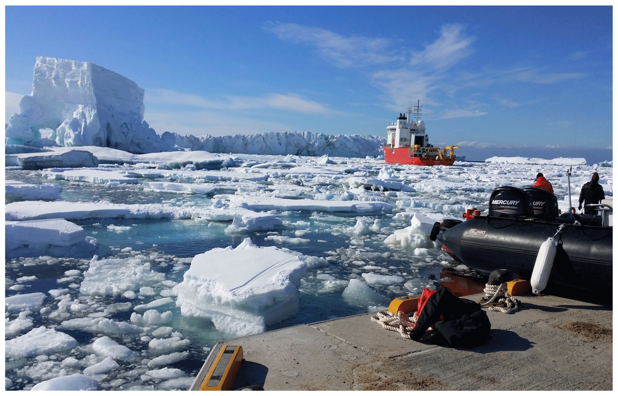
Figure 1Drifting ice, including icebergs and mobile sea ice, around the Jang Bogo Antarctic Research Station (JBARS), photographed on 29 January 2017.
Floating ice shelves occupy around 75 % of Antarctica's perimeter (Padman et al., 2018). Tidal oscillations at the ice–ocean interface influence the location and extent of grounding zones (Padman et al., 2002), and control heat transfer and ocean mixing in cavities beneath the marine cryosphere (Padman et al., 2018) and the calving and drift of icebergs (Rignot et al., 2000). Tides also affect variability in polynyas, seasonal sea ice patterns, and thus the functioning of marine ecosystems. In addition, tides affect the dynamics of landfast sea ice, which provides aircraft landing zones (Han and Lee, 2018).
Accurate Antarctic region tide data are needed for models examining changes in global climate and ocean circulation (Han and Lee, 2018), while coastal tide data are needed for ice mass balance and motion studies (Padman et al., 2008; Rignot et al., 2000; Rosier and Gudmundsson, 2018). Ice thickness is typically measured by subtracting tidal heights from highly accurate but relatively low resolution (temporally or spatially) satellite or in situ observations of ice surface elevation (Padman et al., 2008). Where ice shelves and glacier tongues occur, grounding zone and ice flexure mechanics make ice thickness and motion determination challenging, so that accurate tidal height inputs are crucial (Wild et al., 2019).
In this study, we tested the applicability of Byun and Hart's (2015) CTSM + TCC method in an extreme observation environment using 25 h short-term records from JBARS, our temporary tidal observation station, and year-long data from ROBT, the neighbouring reference station. Section 2 of this paper details the JBARS and ROBT observation data sets used to generate harmonic tidal analysis results and CTSM + TCC tidal predictions. Section 3 explains how the CTSM + TCC method was applied and adapted in this case study (with Appendix A detailing the calculations), while Sect. 4 demonstrates the CTSM + TCC tidal prediction capability. Section 5 discusses the generation of fortnightly tide effects and double tidal peaks; and situates the Ross Sea tides examined in this paper within the wider context of Antarctic tidal regimes.
2.1 Study sites and data records
The Korea Hydrographic and Oceanographic Agency (KHOA) survey team went to JBARS in northern Victoria Land's Terra Nova Bay, Ross Sea, Antarctica, in the austral summertime of 2017 (Fig. 2) for a preliminary field trip to conduct hydrographic surveys and produce a nautical chart. This mission collected the first 19 d sea-level-related record for JBARS: 10 min interval subsurface pressure observations were recorded between 28 January and 16 February 2017 using a bottom-mounted absolute pressure sensor (WTG-256S AAT, Republic of Korea) with the data converted to equivalent sea level heights using the hydrostatic equation. High-frequency sea level oscillations (<3 h) were removed from the observation record using a fifth-order low-pass Butterworth filter. Note that the first and last days of this campaign comprised partial-day records, so we excluded these end days from our tidal prediction experiments, since our method requires continuous 25 h input data (i.e. covering one tidal cycle minimum and, for convenience, starting at midnight). That left 17 d and 1 h of useable tidal observation data as the basis of the primary JBARS observation record. Note that short-term records >25 h may be used in CTSM + TCC but, as demonstrated in Byun and Hart (2015), large tidal range (range being twice the amplitude) and high data quality have a much greater positive impact on prediction results than any increase in the length of the short-term observation records employed.
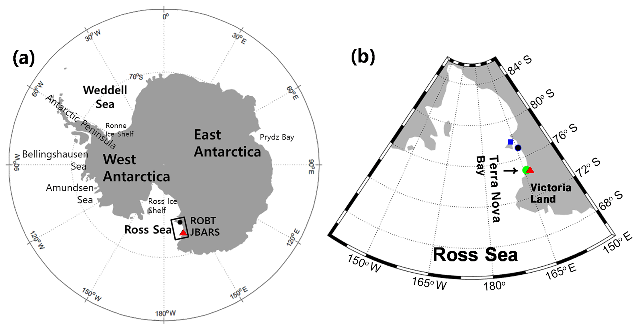
Figure 2Maps showing (a) the locations of the two tidal observation
stations employed in this study within a wider Antarctic context: Jang Bogo
Antarctic Research Station (JBARS, ![]() )
and Cape Roberts (ROBT,
)
and Cape Roberts (ROBT, ![]() ); (b) the
case study station locations relative to two other (previous) temporary
tidal observations stations, McMurdo Station (
); (b) the
case study station locations relative to two other (previous) temporary
tidal observations stations, McMurdo Station (![]() )
and Mario Zucchelli Station
(
)
and Mario Zucchelli Station
(![]() ),
in the Ross Sea.
),
in the Ross Sea.
For the purposes of a full-scale survey, three additional discontinuous sea level observation records were measured by KHOA at JBARS between 29 December 2018 and 11 March 2019, all at 10 min intervals using the same instrument. Of these, the 20.54 d record produced between 29 December 2018 and 18 January 2019 comprised relatively high-quality data with small residuals (i.e. observations minus predictions). We used this additional data set (hereafter referred to as the JBARS 2019 observations) to verify CTSM + TCC method tidal predictions generated from input parameters derived from “daily” (25 h) slices of the 2017 sea level records. Due to the short duration of the KHOA survey team's forays into the Ross Sea, and in the absence of a permanent tide station at JBARS, it was not possible to collect the year-long sea level records that are commonly employed to obtain reliable tidal harmonic constants for tidal prediction.
Approximately 269 km south of JBARS, there is a permanent tidal observation station named after its location on ROBT, operated by Land Information New Zealand (LINZ) and recording at intervals since November 1990 (Fig. 2). The 5 min interval seawater pressure data have been collected at ROBT since November 2011 using GEOKON 4500 series standard piezometers, vented to the atmosphere, with these data converted to sea level heights using the hydrostatic equation. Part of the 2017 record from this site was unavailable online at the time of starting this research, so instead we chose as our reference records the 2013 ROBT sea level data, a quality year-long data set with few missing points.
2.2 Tidal characteristic analyses and descriptions
Using the T_TIDE toolbox (Pawlowicz et al., 2002), we obtained the tidal harmonic constants of the eight and six major tidal constituents for ROBT and JBARS, respectively (Table 1). Also the inference method was used to infer the P1 constituent from the K1, and the K2 constituent from the S2, with their amplitude ratios and phase lag differences obtained from harmonic analysis of the long-term ROBT reference station records. Analyses revealed that the two main diurnal (O1 and K1) and semidiurnal (M2 and S2) tides had similar amplitudes at the two stations, with the diurnal (semidiurnal) amplitudes being slightly larger (smaller) at ROBT than at JBARS, and the phase lags of all four tides having only slightly different values at the two stations. The amplitude differences result in slightly different tidal form factors at the two sites (e.g. F in Table 1).
Table 1Major tidal harmonic results for diurnal and semidiurnal constituents from harmonic analyses of sea level observations: the year-long (2013) record from ROBT, and 17.04 d record (29 January to 15 February 2017) and 20.54 d record (29 December 2018 to 18 January 2019) from JBARS in the Ross Sea (see source details in Sect. 2). For the JBARS tidal harmonic analyses, the inference method was used to infer the P1 constituent from the K1, and the K2 constituent from the S2, with their amplitude ratios and phase lag differences obtained from harmonic analysis of the long-term ROBT 2013 reference station record.
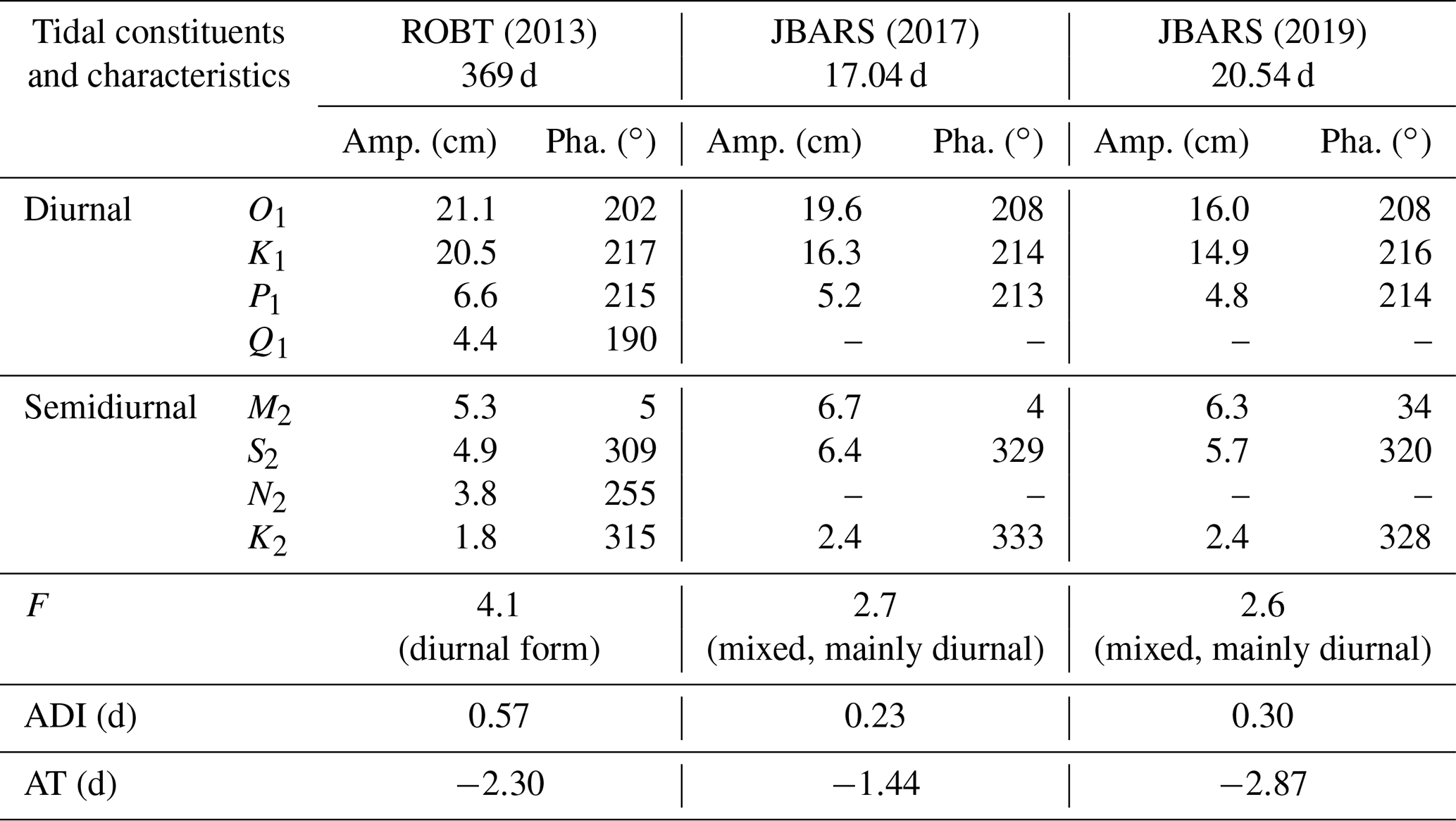
Note: amp. denotes amplitude; pha. denotes phase lag, referenced to 0∘ Greenwich; F is the amplitude ratio of the ( tides; and ADI and AT denote the age of diurnal inequality and the age of the tide.
Having analysed the tidal harmonic constants at the two stations, we then employed the CTSM + TCC method (Byun and Hart, 2015) to generate tidal height predictions for JBARS, our “temporary” tidal observation station (subscript o), using ROBT as the “reference” station (subscript r). This prediction approach (see Appendix A for the detailed calculations, and Byun and Hart (2015) for explanation of procedure development) is based on
- i.
using long-term (1 year, in our case) reference station records (LHr) and CTSM calculations to make an initial anytime (τ) tidal prediction (ηr(τ)), which involves summing tidal species' heights for the reference station (Fig. 3);
- ii.
comparing the tidal harmonic constants (amplitude ratios and phase lag differences) of representative tidal constituents (e.g. M2 and K1) for each tidal species between the temporary and reference stations (Fig. 4), calculated using T_TIDE and concurrent short-term records (≥25 h duration, starting at midnight) from the temporary (SHo) and reference (SHr) stations; and
- iii.
using the step (ii) comparative data and the TCC calculations for each tidal species to adjust the ηr(τ) tidal species' heights in order to generate accurate, anytime tidal height predictions for the temporary tidal station (ηo(τ)).
In this Ross Sea case study, we used the 2017 JBARS tidal observation records (i.e. 17.04 d from 00:00 29 January to 01:00 UTC 15 February) as a source of SHo, keeping the second JBARS 2019 observation record for evaluation purposes.
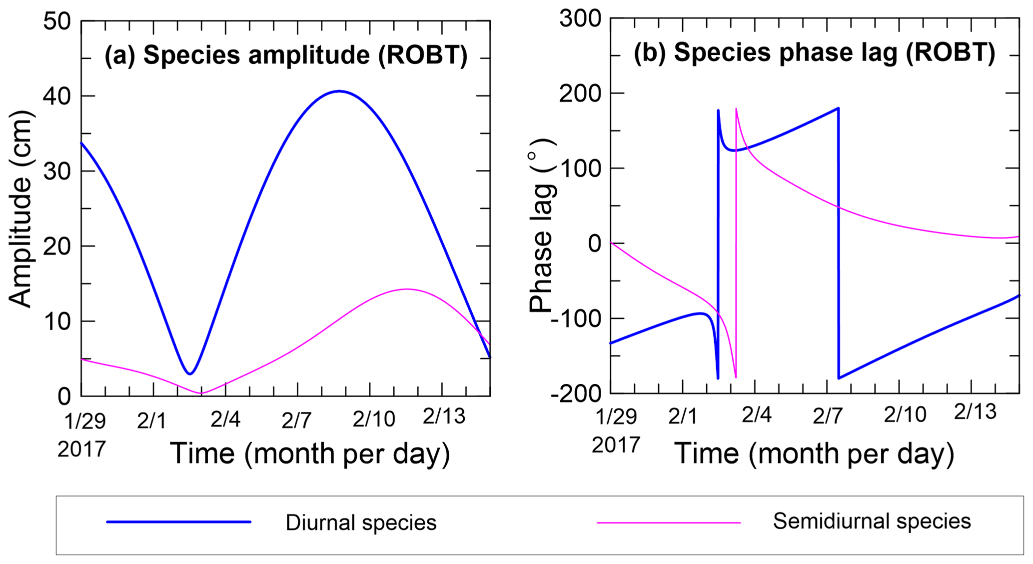
Figure 3Modulated tidal (a) species amplitudes and (b) phase lags for the diurnal and semidiurnal tidal species, calculated from ROBT tidal prediction data (29 January to 14 February 2017), using Eqs. (A1) and (A3) in Appendix A. Throughout the figures, dates are displayed in mm/dd format.
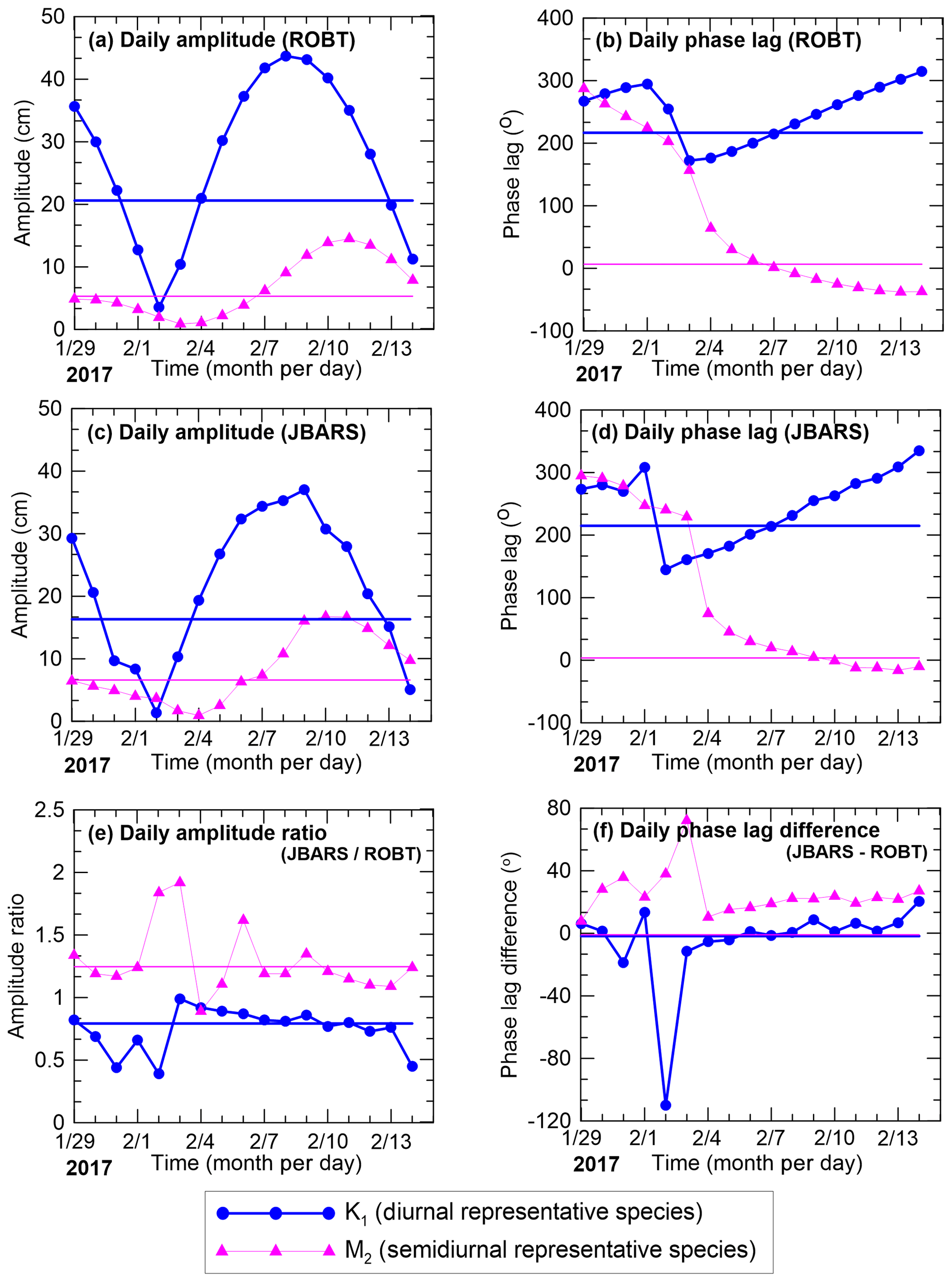
Figure 4Daily amplitudes (a, c); phase lags (b, d); amplitude ratios (e); and phase lag differences (f) of the K1 and M2 tides (representative diurnal and semidiurnal tide species) at ROBT (a, b) and JBARS (c, d), and between JBARS and ROBT (e, f), calculated from “daily” slices of the 29 January to 14 February 2017 ROBT tidal predictions and JBARS sea level observations. In addition, thick blue (K1) and thin pink (M2) horizontal lines in the panels indicate the amplitudes and phase lags derived from harmonic analyses of the entire 369 d 2013 ROBT sea level record (a, b) and of the entire 17 d 2017 JBARS sea level record (c, d), along with their amplitude ratios and phase lag differences (e, f).
Importantly, this method assumes that the reference and temporary tidal stations are situated in neighbouring regimes with similar dominant tidal constituent and tidal species characteristics, and that the tidal properties between the two stations remain similar through time. As explained above, both JBARS and ROBT have tidal regimes that are primarily dominated by diurnal tides. LHr can come from any time period but must comprise high-quality (e.g. few missing data) tidal height observations throughout.
Byun and Hart (2015) recommended the use of short-term records gathered during periods of calm weather to minimise errors due to atmospheric influences. They employed observational data for both SHo and SHr, but as demonstrated in this paper the method can also be applied using tidal predictions as a source of SHr. This adjustment in approach arose since, for the 2017 JBARS observation time period, the concurrent 2017 ROBT records available online (LINZ, 2019) had multiple missing data. We solved this issue by producing a year-long synthetic 2017 record for ROBT using T_TIDE (Pawlowicz et al., 2002) and the 2013 (i.e. LHr) observational record as input data. The 17.04 d of predicted tides that were concurrent with the 2017 JBARS observation record were then used as our SHr source. While this CTSM + TCC method adjustment was procedurally small, it represents an important adaptation in the context of generating tidal predictions for stations situated in extreme environments, since concurrent temporary and reference station observations might be rare in such contexts.
When using CTSM + TCC, if the available temporary tidal station observation record covers multiple days, it is best practice to experiment by generating multiple ηo(τ), each using different concurrent pairs of SHo and SHr daily data slices in step (ii) above, to produce daily amplitude ratios and phase lag differences between the two stations for the diurnal K1 and semidiurnal M2 tidal constituents. Comparisons are then made between the different ηo(τ) data sets produced and the original temporary station observations to determine the optimal 25 h window to use: once selected, tidal height predictions can be generated for the temporary observation station for any time period. Thus, 17 individual 25 h duration data slices were clipped from the 2017 JBARS observation records and from the concurrent ROBT predictions, forming 17 pairs of SHo and SHr “daily” slices. Each paired data set was then used with LHr to generate tidal height predictions for JBARS covering both the 2017 and 2019 KHOA observation campaign time periods. Comparisons were made between the complete JBARS observations and the 17 prediction data sets generated for each campaign to identify which 25 h short-term data window produced optimal ηo(τ) results.
4.1 Tidal prediction evaluation
CTSM+TCC was used to produce 17 different JBARS tidal prediction data sets for the period 29 January to 14 February 2017, based on harmonic analysis results of the “daily” (25 h) K1 and M2 amplitudes and phase lags at our two tidal observation stations. Figure 5a illustrates one such tidal height prediction data set, in comparison to the observed tides. In order to evaluate the 17 different prediction results, each prediction data set was compared with the concurrent JBARS field observations via root mean square error (RMSE) and coefficient of determination (R2) statistics.
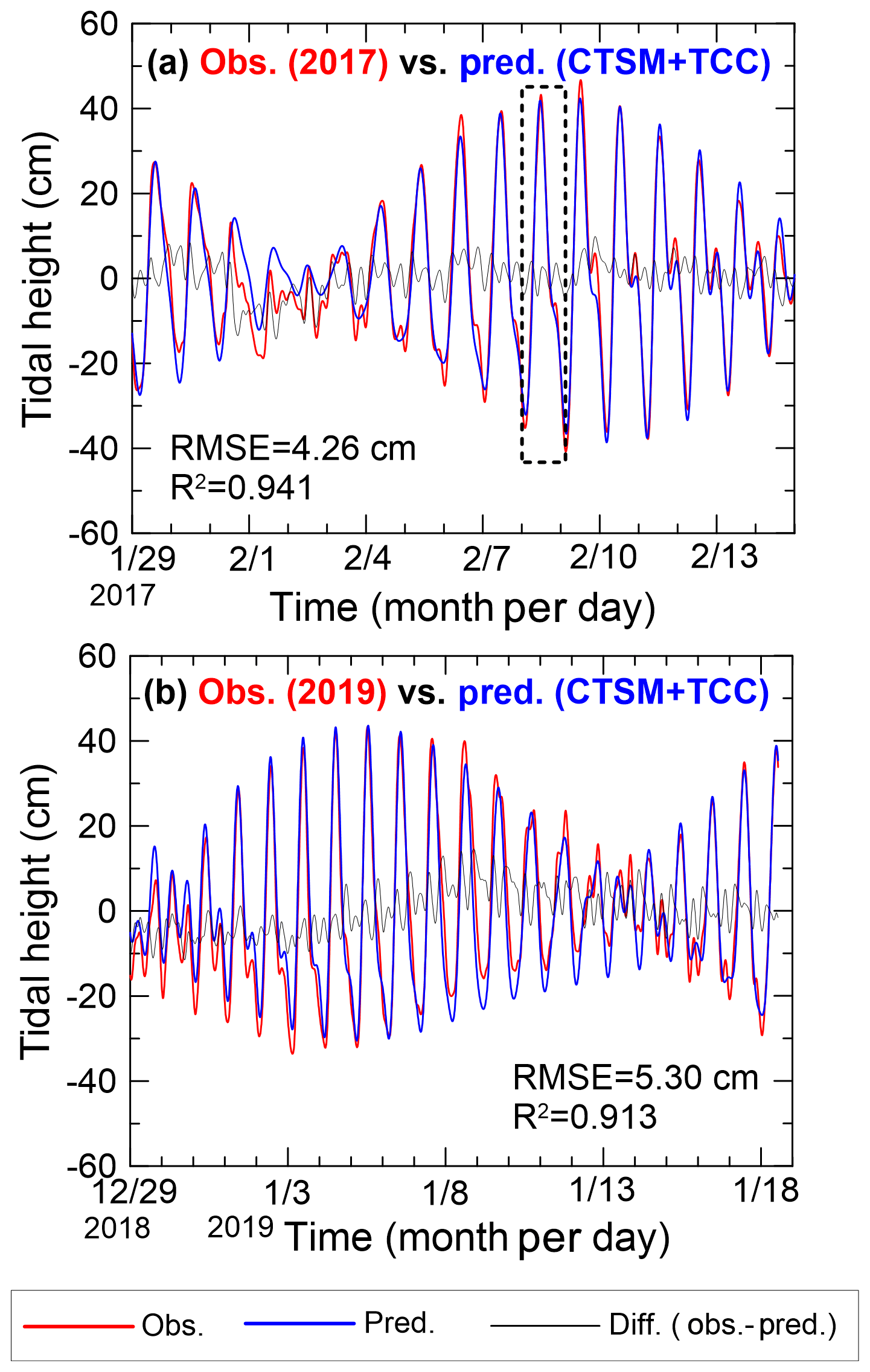
Figure 5Time series of JBARS sea level observations (obs.), predicted tidal heights (pred.), and sea level residuals (diff.) from (a) 29 January to 14 February 2017; and (b) 29 December 2018 to 18 January 2019. The JBARS predictions were generated via the CTSM + TCC method using a daily (25 h) slice of local sea level observations from 8 February 2017 (dashed box in panel a), along with concurrent (to time periods a and b) ROBT predictions; and year-long (2017) 5 min interval ROBT tidal predictions. RMSE and R2 denote the comparison root mean square errors and coefficients of determination, respectively.
RMSEs between the 2017 observations and predictions ranged from 4.26 to 20.56 cm, while R2 varied from 0 to 0.94, across the 17 “daily” experiments (Fig. 6). Overall, 11 of the experiments produced accurate results (i.e. excluding those derived from 31 January, and 1–4 and 14 February data slices). Daily data sets from periods with relatively high tidal ranges (>83.5 cm) produced predictions with RMSEs <5 cm and R2 values >0.92. The maximum tidal range occurred on 9 February, with step (ii) data slices from this date producing predictions with a low (but not the lowest) RMSE (4.81 cm). The predictions with the lowest RMSE (4.26 cm) and highest R2 value (0.941) were produced using data slices from 1 d earlier, 8 February 2017 (Figs. 5a and 6). In contrast to the successful prediction data sets, the data set generated using the 2 February 2017 data slices (in step ii of the method) produced predictions with very high RMSE (20.56 cm) and very low R2 (0.00) values (Fig. 6). The 2 February 2017 tides were characterised by the smallest tidal range (11.95 cm) of the JBARS record during a period of low lunar declination.
Interestingly, RMSEs and R2 values between the 2019 CTSM + TCC tidal predictions and observations were almost identical to those of the 2017 comparisons, revealing that our approach performed consistently across different prediction years.
As in the 2017 experiments, the 2019 prediction data set made using the 8 February 2017 data slices (i.e. in step ii of the method) produced the lowest RMSE (5.3 cm) and highest R2 (0.913) values of the 2019 experiments (Fig. 5b).
Across both the 2017 and 2019 prediction time periods, the RMSE and R2 results varied in relation to the JBARS tidal range, with greater accuracy evident in predictions made using step (ii) 2017 data slices from periods with above-average tidal ranges. In the JBARS area of the Ross Sea during the 2017 short-term observation period, above-average tidal ranges corresponded to the period when the Moon was near its greatest northern declination (Fig. 6).
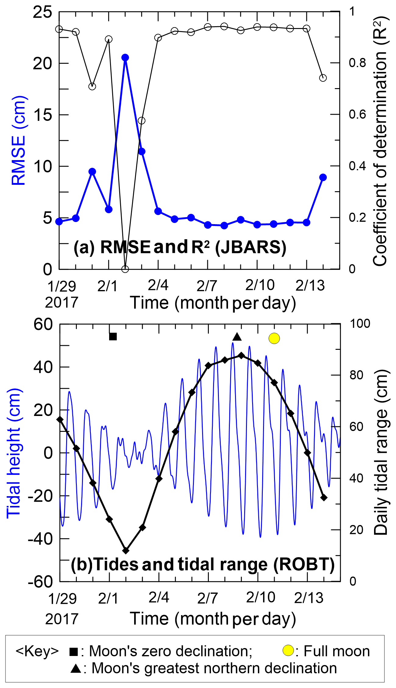
Figure 6(a) Time series (29 January to 14 February 2017) of RMSEs
(thick blue line with ![]() )
and coefficients of determination (R2,
thin black line with
)
and coefficients of determination (R2,
thin black line with ![]() )
between JBARS 10 min interval sea level
observations and the CTSM + TCC prediction data sets, generated for this site
using harmonic analysis results from the JBARS daily (25 h) sea level data
slices and concurrent daily (25 h) 2017 tidal prediction data slices and
harmonic analysis results from ROBT station's year-long (2017) tidal
predictions. (b) Time series of predicted 2017 tidal heights (thin blue
line) and daily tidal ranges (thick black line with
)
between JBARS 10 min interval sea level
observations and the CTSM + TCC prediction data sets, generated for this site
using harmonic analysis results from the JBARS daily (25 h) sea level data
slices and concurrent daily (25 h) 2017 tidal prediction data slices and
harmonic analysis results from ROBT station's year-long (2017) tidal
predictions. (b) Time series of predicted 2017 tidal heights (thin blue
line) and daily tidal ranges (thick black line with ![]() ) for
ROBT, based on harmonic analysis of this station's 2013 5 min interval sea
level record, plus an indication of the Moon's phase and declination.
) for
ROBT, based on harmonic analysis of this station's 2013 5 min interval sea
level record, plus an indication of the Moon's phase and declination.
Collectively, these results show that the CTSM + TCC method can be used successfully to predict tidal heights for JBARS, when using short-term observation records gathered from periods at high lunar declination, and thus above-average tidal ranges, with relatively calm weather, together with observation or prediction records from the neighbouring reference station ROBT.
4.2 Determining the ideal short-term sea level observation period when using CTSM + TCC
The previous section verified that the CTSM + TCC method can be used to generate accurate tidal predictions based on 25 h sea level records, from periods with above-average tidal ranges, for a temporary station in a mixed, mainly diurnal regime and a reference station in a diurnal regime. The question arises as to how to determine optimal observation days in such settings to produce the most accurate tidal predictions.
For semidiurnal or mixed, mainly semidiurnal tidal regimes, we can estimate preferred temporary station observation days, those with the largest tidal ranges, based on the Moon's phase, without reference to tide tables. That is, spring tides commonly occur just a day or two after the full and new Moon, which reoccurs at a period of 14.76 d. The time lag between the full or new Moon and the spring tide is called the age of the tide (AT).
Similarly, in a diurnal tide regime or a mixed, mainly diurnal tide regime, preferred temporary station observation days can be estimated based on the lunar declination (Fig. 7), which varies at a period of 13.66 d. That is, maximum tidal range days can be estimated for JBARS based on the day of the Moon's greatest northern (GN) and southern (GS) declinations. The time between the Moon's semi-monthly GN and GS declinations and their effects on tidal range, called the age of diurnal inequality (ADI), is commonly 1 to 2 d. The GN and GS lunar declinations during our temporary station summertime observation periods occurred on 8 February 2017 (GN) and on 6 January 2019 (GS), respectively (Fig. 7), with the maximum diurnal tides at JBARS expected around 1 d after each lunar declination peak.
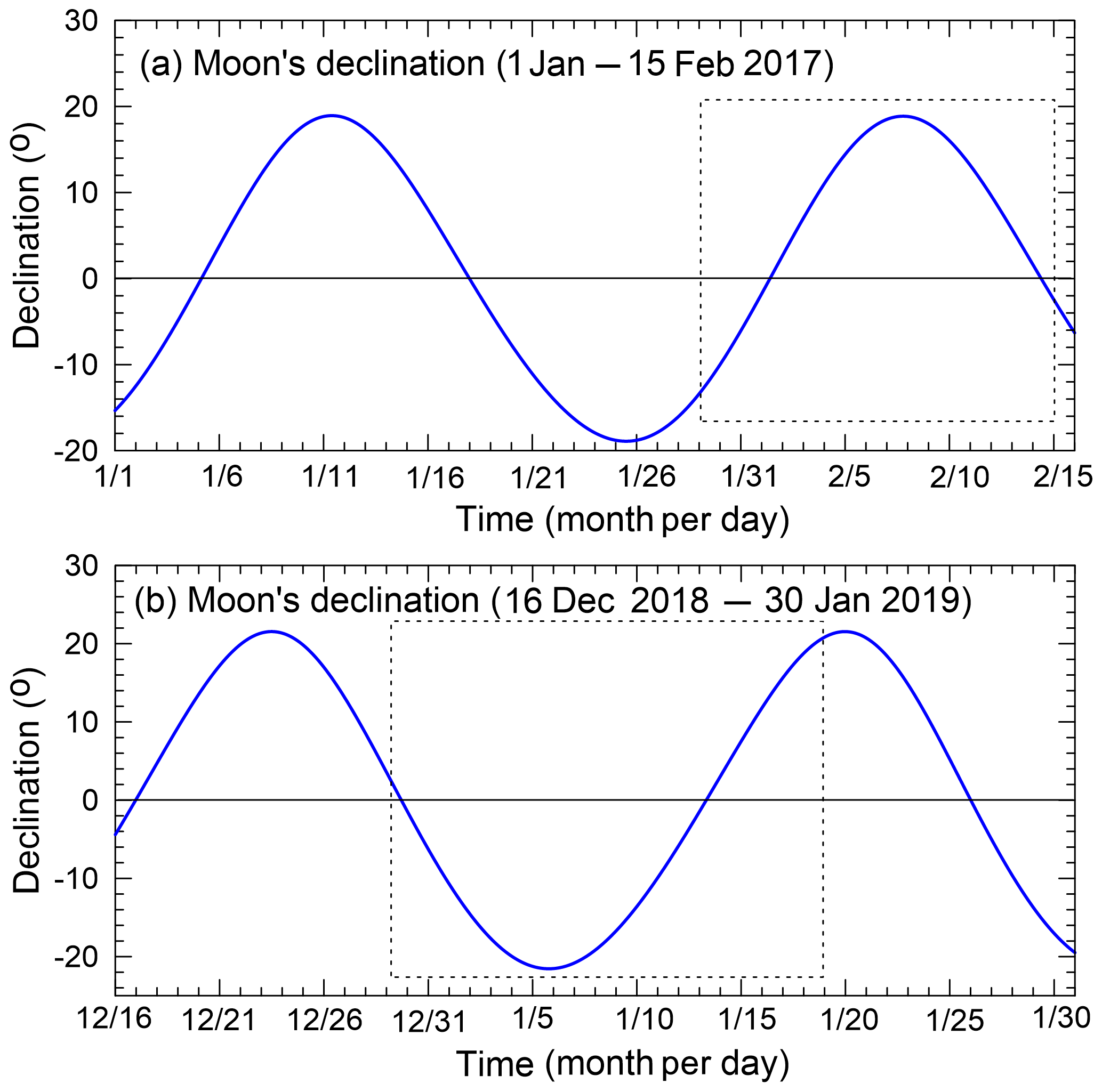
Figure 7Time series of the Moon's declination, calculated at daily intervals for two observation periods: (a) 1 January to 15 February 2017; and (b) 16 December 2018 to 30 January 2019. Dashed boxes indicate the sea level observation windows examined in this study.
Thus, when planning to use the CTSM + TCC tidal prediction method for places characterised by diurnal or mixed, predominantly diurnal tidal regimes, we can use knowledge of the Moon's declination to select potential sea level observation days.
4.3 Comparison of ROBT and JBARS tidal species characteristics
The CTSM + TCC tidal prediction method is based on the assumption that the tidal harmonic characteristics of each tidal species are very similar between the temporary and reference stations. This is because the reference station tidal species' CTSMs form the basis of the tidal predictions for the temporary observation station. To test the validity of this assumption, we examined the phase lag (G) differences of the two major diurnal and semidiurnal tidal constituents using ADI and AT, calculated as
where (= 15.0410686∘ h−1), (= 13.9430356∘ h−1), (= 30.0000000∘ h−1), and (= 28.9841042∘ h−1) are the angular speeds of the K1, O1, S2, and M2 tides, respectively. Results revealed that the ADI are very similar, and there is <1 d AT difference, between ROBT and JBARS, respectively (Table 1), indicating that the tidal characteristics of the representative tidal constituents for each species between the two stations are very similar, in particular the dominant diurnal species. Note that the negative AT values in Table 1 are an unusual feature of the Ross Sea tides, given that elsewhere spring tides commonly occur a day or two after the full and new Moon. The ADI and AT similarities between our two stations explain why we found the CTSM + TCC method successful in generating the Ross Sea tidal predictions.
5.1 Explaining fortnightly tide effects and double tide peaks in the Ross Sea tidal predictions
We have demonstrated that the CTSM + TCC approach can produce reasonably accurate tidal predictions (RMSE < 5 cm, R2>0.92) for a new site in the Ross Sea, Antarctica, based on 25 h temporary station observation records from periods with above-average tidal ranges, plus neighbouring reference station records. Our results compare favourably with those of Han et al. (2013), who reviewed the tidal height prediction accuracy of four models for Terra Nova Bay, Ross Sea: these models generated similar quality results to our CTSM+TCC results, with R2 values between 0.876 and 0.907, and RMSEs ranging from 3.6 to 4.1 cm. However, as shown in Fig. 5, our results contain a changing fortnightly timescale bias in estimates. This error pattern likely resulted from our application of CTSM + TCC considering only two major tidal species (diurnal and semidiurnal) whilst ignoring several long-period and small-amplitude short-period tides.
Table 2Harmonic constants for six long-period tidal constituents, derived from harmonic analysis of a 1-year-long observation (2013) measured at the ROBT sea level gauge, using T_TIDE (Pawlowicz et al., 2002). Note that this gauge is a vented piezometer so caution should be exercised in interpreting the results (particularly for Sa and Ssa) given the inclusion of proportionately large non-tidal (atmospheric) variations in this kind of sea level record.
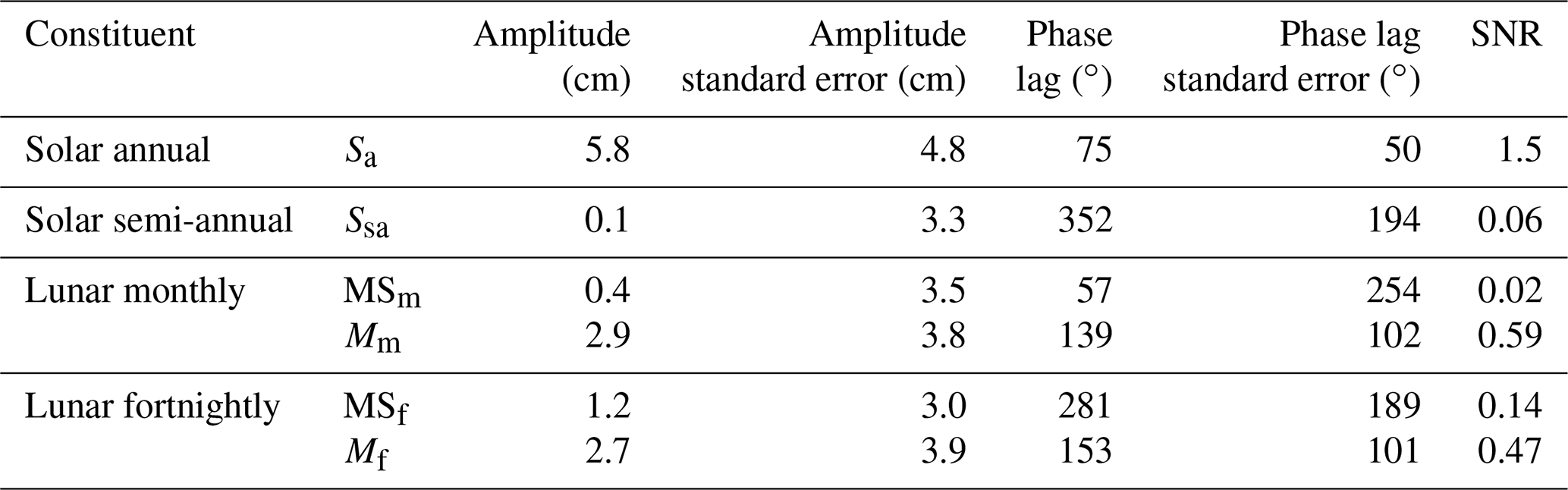
Phase lags are referenced to 0∘ Greenwich, and SNR denotes the signal-to-noise ratios.
Table 2 summarises the characteristics of six long-period tides (Sa, Ssa, MSm, Mm, Mf, MSf) at the ROBT station, derived from tidal harmonic analysis of year-long (2013) in situ observation records. Note that since the ROBT observation record was derived from a differential (vented) pressure sensor, and thus it includes proportionately large non-tidal (atmospheric) sea level variations, caution should be exercised in comparing the harmonic analysis results of the non-astronomical constituents, which are affected by atmospheric (air pressure) forcing (i.e. Sa and Ssa).
To investigate the main cause of the apparent fortnightly prediction biases in our results, we examined the effects of two fortnightly tidal constituents (Mf and MSf) at ROBT using T_TIDE. Three 2019 tidal prediction experiments were conducted:
-
Srun excluded all long-period tides (see list of exclusions in Table 2);
-
Run1 was based on Srun but also incorporated Mf; and
-
Run2 was based on Srun but also incorporated Mf and MSf;
with T_TIDE predictions made for each case. Comparisons between Run1 and Srun predictions revealed that exclusion of the Mf tide (2.7 cm amplitude) can produce prediction biases during periods of lunar declination change, with comparisons between Run2 and Run1 results revealing that the additional exclusion of the MSf tide (1.2 cm amplitude) intensifies the biases. These results elucidate one particular issue to do with long-period tides when predicting Ross Sea tides based on the diurnal and semidiurnal species alone. We note that the aforementioned differences in gauge records (subsurface pressure or real sea level) introduce another. That is, while the diurnal and semidiurnal tides might be considered to be measured equivalently accurately, the longer-period components are expected to be instrument dependent and so have uncertainties for the above experiments.

Figure 8Time series (29 December 2018 to 18 January 2019) of (a) predictions of the diurnal (K1+O1) tides (blue line) and the semidiurnal (M2+S2) tides (magenta line) for JBARS; (b) their combined JBARS predictions (red line) and observations (dashed black line); (c) the ROBT diurnal (blue line) and semidiurnal (magenta line) species amplitudes and their ratio (green line); and (d) the ROBT diurnal (blue line) and semidiurnal (magenta line) species phase lags and their difference (diurnal – semidiurnal) (green line).
Rosier and Gudmundsson (2018) found that ice flows are modulated at various tidal frequencies, including that of the MSf tide. However, because these tides' amplitudes have small signal-to-noise ratios (<1) with large standard errors (Table 2), caution should be exercised when elucidating fortnightly tide effects using these constituents. Nevertheless, studies indicate that incorporating major and minor tidal constituents, including long-period tides, into tidal predictions may be advantageous for their use in ice flow and ice–ocean front modelling specifically (e.g. Rignot et al., 2000; Rosier and Gudmundsson, 2018). Consideration of additional, long-period tides in predictions is one recommendation we have for future work on improving tidal predictions for Ross Sea coasts.
Another characteristic of our results needing explanation is the double tidal peaks evident in both the tidal observations and predictions at JBARS. These peaks occur, for example, in Fig. 5b between 11 and 17 January 2019. To explore why these double peaks occur, we generated JBARS tidal height predictions using Eq. (A1) in Appendix A and the 2019 tidal constants listed in Table 1 for the two major diurnal and semidiurnal tides. Figure 8a shows separately the resulting diurnal (with their period of 13.66 d) and semidiurnal (with their period of 14.77 d) species' tide predictions. The combination of these out-of-phase tidal species generates double peaks (or double troughs) around low and high tide (Fig. 8b) for periods when the diurnal tide amplitude is low, due to the similar amplitude K1 and O1 tides cancelling each other out across a fortnight, allowing the combined M2 and S2 amplitude to temporarily approach or exceed that of the combined K1 and O1 tides (Fig. 8c). Since the semidiurnal tides are slightly stronger, and the diurnal tides are slightly weaker, at JBARS compared to at ROBT (Table 1), these double tide peaks occur more commonly at JBARS.
5.2 Understanding the contrasting tidal environments around Antarctica
Figure 9 illustrates the form factors of tidal regimes in the seas surrounding Antarctica, according to Finite Element Solution 2014 (FES2014) model data. There are large areas characterised by diurnal (F>3); mixed, mainly diurnal (); and mixed, mainly semidiurnal () forms. Only in a small area halfway along the Weddell Sea coast of the Antarctic Peninsula (at 72∘ S) do tides exhibit a semidiurnal form (F<0.25). The Weddell Sea is dominated by mixed, mainly semidiurnal tides, with the exception of the semidiurnal area mentioned and another small area exhibiting diurnal tides (F>3) at around 76.5∘ S, where amphidromic points (i.e. zero amplitudes) occur for both the M2 and S2 tides. Strong diurnal tides predominate in the Ross Sea area of West Antarctica, to around the Amundsen Sea. In addition, a small area near Prydz Bay (Fig. 2) in East Antarctica exhibits diurnal and mixed mainly diurnal tides. The rest of the seas surrounding Antarctica are predominantly characterised by mixed, mainly semidiurnal tides.

Figure 9Distribution of tidal form factor (F) values around Antarctica. Note the magenta area (72∘ S) on the Antarctic Peninsula's Weddell Sea coast denotes the only area with a properly semidiurnal tide regime (F<0.25) in the Antarctic region.
Since diurnal tides have larger nodal amplitude factors and nodal angle variations than semidiurnal tides (Pugh and Woodworth, 2014), areas like the Ross Sea will have larger variations in tidal height across the 18.61-year lunar nodal cycle compared to areas like the Weddell Sea. As the nodal amplitude factor variations of the diurnal and semidiurnal tides are out of phase, this leads to differing tidal responses around Antarctica over 18.61 years, particularly between the Ross and Weddell seas (see details of ROBT in Byun and Hart, 2019). Given that CTSM + TCC is based on modulated tidal amplitude and phase lag corrections for each diurnal and semidiurnal species, this approach is applicable in studying a continent with such a diversity of tidal regime types.
This paper has demonstrated the usefulness of the CTSM + TCC method for tidal prediction in extreme environments, where long-term tidal station installations are difficult, using the Ross Sea in Antarctica for our case study. Here, CTSM + TCC methods can be employed for accurate tidal height predictions for a temporary tidal observation station using short-term (≥25 h) sea level records from this site, plus long-term (1-year) tidal records from a neighbouring reference tidal station. Essentially, the temporary and reference station sites must share similarities in their main tidal constituent and tidal species characteristics for CTSM + TCC to produce acceptable results.
Using this approach, an initial tidal prediction time series is generated for the temporary station using CTSM and the reference station long-term records. The temporary station predicted time series can then be adjusted via TCC of each tidal species, based on harmonic comparisons between the short-term temporary station observation record and its corresponding modelled predictions, leading to improved accuracy in the tidal predictions. The modulated amplitude ratio and phase lag difference between diurnal and semidiurnal species predicted from CTSM at the reference station can be used as an indicator for selecting optimal short-term observation dates at a temporary tidal station.
This paper has further demonstrated that the CTSM + TCC approach can be employed successfully in the absence of concurrent short-term (25 h) records from the reference station, since a tidal harmonic prediction programme can be used to produce a synthetic short-term record for the reference station, based on a quality long-term (1-year) record from that site.
The proper consideration of long-period tides in the CTSM + TCC approach remains a challenge, as outlined in this study, with the solutions to this issue likely to improve tidal predictions further. However, this study demonstrates that the CTSM + TCC method can already produce tidal predictions of sufficient accuracy to aid local polar station maritime operations, as well as starting to help resolve gaps in the spatial coverage of tidal height predictions for scientists studying important issues, such as the rate and role of ice loss along polar coastlines.
This appendix describes the calculations involved in using the CTSM + TCC approach as employed in this Ross Sea, Antarctica, case study. For a fuller description of the development of this approach and its application in semidiurnal and mixed, mainly semidiurnal tidal regime settings, see Byun and Hart (2015).
As explained in the main body of this paper, we used 25 h slices of the 2017 short-term observations from JBARS (SHo), our temporary tidal observation station (subscript o), and 2013 year-long observations (LHr) and 2017 short-term tidal predictions (SHr, concurrent with SHo) from ROBT, our reference tidal station (subscript r), as the basis of JBARS tidal prediction calculations. We then employed the full 17.04 d 2017 JBARS tidal observation data set, and an additional 21.54 d 2019 JBARS tidal observation data set, to evaluate the success of the CTSM + TCC tidal prediction calculations for this site.
The CTSM + TCC, expressed as the summation of each tidal species cosine function, includes three key steps:
- i.
calculating each tidal species' modulation at the reference tidal station;
- ii.
comparing the tidal harmonic constants between the temporary observation and reference stations (e.g. the tidal amplitude ratios and phase lag differences of each representative tidal constituent for each tidal species calculated from concurrent observation records between two stations); and
- iii.
adjusting the tidal species modulations calculated in the first step using the correction factors calculated in the second step to produce predictions for the temporary tidal station.
As a first step, tidal height predictions for the temporary station (ηo(τ)) were initially derived from reference station predictions (ηr(τ)) on the assumption that the tidal properties between the two stations remain similar through time. Using the modulated amplitude () and the modulated phase lag () for each tidal species, this step is expressed as
with
and
where superscript s denotes the type of tidal species (e.g. 1 for diurnal species and 2 for semidiurnal species); m is the number of tidal constituents; t0 is the reference time; t is the time elapsed since t0; and ; indicates the angular frequencies of each tidal constituent (subscripts i and j); indicates the angular frequencies of each tidal constituent representing a tidal species (subscript R); with the dominant tidal constituent of each tidal species used as the representative for that species (e.g. K1 and M2 are used as representative of the diurnal and semidiurnal species, respectively). For each tidal constituent, and are the tidal harmonic amplitudes and phase lags (referenced to Greenwich); is the nodal amplitude factor of each tidal constituent; is the nodal angle; and is the astronomical argument. T_TIDE was used for tidal harmonic analysis as well as for calculation of the nodal amplitude factors, nodal angles, and astronomical arguments, for the representative tidal constituents.
As the second step, under the “credo of smoothness” assumption that the admittance or “ratio of output to input” does not change significantly between constituents of the same species (Munk and Cartwright, 1966; Pugh and Woodworth, 2014), the amplitude ratio and phase lag difference of each representative tidal constituent for each tidal species between the temporary and reference stations were calculated from the results of tidal harmonic analyses of concurrent 25 h data slices (starting at 00:00 UTC) from the temporary observation and reference tidal stations (i.e. from SHo and SHr). The process of selecting the optimal 25 h window for the concurrent data slices from amongst the 17.04 d of available records is explained in Sect. 3.
Once this 2017 window was selected, the third step involved adjusting the tidal predictions at the reference station calculated from Eq. (A1), to represent those for the temporary station (ηo(τ)), by substituting the daily (i.e. SHo and SHr) amplitude ratios and phase lag differences for the tidal constituents (K1 and M2) representing the diurnal and semidiurnal tidal species between the temporary and reference stations into Eq. (A1) as follows (Byun and Hart, 2015):
Substituting Eqs. (A5) and (A6) into Eq. (A4), ηo(τ) can be expressed as
The T_TIDE-based CTSM code is available from https://au.mathworks.com/matlabcentral/fileexchange/73764-ctsm_t_tide (last access: 16 September 2020).
The T_TIDE-based CTSM code is available from https://au.mathworks.com/matlabcentral/fileexchange/73764-ctsm_t_tide (Byun, 2019).
The sea level data used in this paper are available from LINZ (2019, http://www.linz.govt.nz/sea/tides/sea-level-data/sea-level-data-downloads) for selected ROBT records, with the remaining ROBT records available by email application (customersupport@linz.govt.nz); and the JBARS records used are available on request from KHOA (infokhoa@korea.kr). Details of the FES2014 tide model are found in Carrère et al. (2016) and via https://www.aviso.altimetry.fr/en/data/products/auxiliary-products/global-tide-fes.html (AVISO, 2020).
DSB conceived of the tidal prediction idea behind this paper and drafted initial results sections. Both authors worked on initial and final versions of the full manuscript.
The authors declare that they have no conflict of interest.
This article is part of the special issue “Developments in the science and history of tides (OS/ACP/HGSS/NPG/SE inter-journal SI)”. It is not associated with a conference.
We are grateful to Land Information New Zealand (LINZ) and the Hydrographic Survey Division of the Korea Hydrographic and Oceanographic Agency (KHOA) for supplying the tidal data used in this research. Special thanks are given to Glen Rowe from LINZ for sharing his extensive knowledge of the Cape Roberts sea level gauge site and its records, and to a KHOA colleague for providing the photograph in Fig. 1. Further, we gratefully thank Hyowon Kim at KHOA for her kind assistance with drafting figures. We are also grateful to Philip Woodworth, Glen Rowe, and an anonymous reviewer for comments that greatly helped us improve our manuscript.
This paper was edited by Philip Woodworth and reviewed by Glen Rowe and one anonymous referee.
AVISO: FES (Finite Element Solution) – Global tide, available at: https://www.aviso.altimetry.fr/en/data/products/auxiliary-products/global-tide-fes.html, last access: 16 September 2020.
Byun, D.-S.: CTSM_T_Tide, MATLAB Central File Exchange, available at: https://au.mathworks.com/matlabcentral/fileexchange/73764-ctsm_t_tide (last access: 16 August 2020), 2019.
Byun, D.-S. and Hart, D. E.: Predicting tidal heights for new locations using 25h of in situ sea level observations plus reference site records: A complete tidal species modulation with tidal constant corrections, J. Atmos. Ocean. Tech., 32, 350–371, https://doi.org/10.1175/JTECH-D-14-00030.1, 2015.
Byun, D.-S. and Hart, D. E.: On robust multi-year tidal prediction using T_TIDE, Ocean Sci. J., 54, 685–691, https://doi.org/10.1007/s12601-019-0028-4, 2019.
Carrère, L., Lyard, F., Cancet, M., Guillot, A., and Picot, N.: FES 2014, a new tidal model – validation results and perspectives for improvements, Presentation to ESA Living Planet Conference, 9–13 May 2016, Prague, 2016.
Codiga, D. L.: Unified Tidal Analysis and Prediction Using the UTide Matlab Functions, Technical report 2011-01, Graduate School of Oceanography, University of Rhode Island, 2011.
Foreman, M. G. G.: Manual for Tidal Heights Analysis and Prediction, Pacific Marine Science Report, 77-10, Institute of Ocean Sciences, Patricia Bay, Sidney, B.C., Canada, 1977.
Gandolfi, S.: Terra Nova Bay Permanent Tide Gauge Observatory Site, available at: https://www.geoscience.scar.org/geodesy/perm_ob/tide/terranova.htm (last access: 4 February 2020), 1996.
Han, H. and Lee, H.: Glacial and tidal strain of landfast sea ice in Terra Nova Bay, East Antarctica, observed by interferometric SAR techniques, Remote Sens. Environ., 209, 41–51, https://doi.org/10.1016/j.rse.2018.02.033, 2018.
Han, H., Lee, J., and Lee, H.: Accuracy assessment of tide models in Terra Nova Bay, East Antarctica, for glaciological studies of DDInSAR technique, Korean Journal of Remote Sensing, 29, 375–387, 2013.
Han, S. C., Shum, C. K., and Matsumoto, K.: GRACE observations of M2 and S2 ocean tides underneath the Filchner-Ronne and Larsen ice shelves, Antarctica, Geophys. Res. Lett., 32, L20311, https://doi.org/10.1029/2005GL024296, 2005.
Jourdain, N. C., Molines, J.-M., Le Sommer, J., Mathiot, P., Chanut, J., de Lavergne, C., and Madec, G.: Simulating or prescribing the influence of tides on the Amundsen Sea ice shelves, Ocean Model., 133, 44–55, https://doi.org/10.1016/j.ocemod.2018.11.001, 2018.
King, M. A., Padman, L., Nicholls, K., Clarke, P. J., Gudmundsson, G. A., Kulessa, B., and Shepherd, A.: Ocean tides in the Weddell Sea: New observations on the Filchner-Ronne and Larsen C ice shelves and model validation, J. Geophys. Res., 116, C06006, https://doi.org/10.1029/2011JC006949, 2011.
LINZ (Land Information New Zealand): Sea level data downloads, available at: http://www.linz.govt.nz/sea/tides/sea-level-data/sea-level-data-downloads, last access: 11 November 2019.
Munk, W. H. and Cartwright, D. E.: Tidal spectroscopy and prediction, Math. Phys. Sci., 259, 533–581, https://doi.org/10.1098/rsta.1966.0024, 1966.
Padman, L., Fricker, H., Coleman, R., Howard, S., and Erofeeva, L.: A new tide model for the Antarctic ice shelves and seas, Ann. Glaciol., 34, 247–254, https://doi.org/10.3189/172756402781817752, 2002.
Padman, L., Erofeeva, S., and Joughin, I.: Tides of the Ross Sea and Ross Ice Shelf cavity, Antarct. Sci., 15, 31–40, https://doi.org/10.1017/S0954102003001032, 2003.
Padman, L., Erofeeva, S., and Fricker, H.: Improving Antarctic tide models by assimilation of ICESat laser altimetry over ice shelves, Geophys. Res. Lett., 35, l22504, https://doi.org/10.1029/2008GL035592, 2008.
Padman, L., Siegfried, M., and Fricker, H.: Ocean Tide Influences on the Antarctic and Greenland Ice Sheets, Rev. Geophys., 56, 142–184, https://doi.org/10.1002/2016RG000546, 2018.
Pawlowicz, R., Beardsley, B., and Lentz, S.: Classical tidal harmonic analysis including error estimates in MATLAB using T_TIDE, Comput. Geosci., 28, 929–937, https://doi.org/10.1016/S0098-3004(02)00013-4, 2002.
Pugh, D. T. and Woodworth, P. L.: Sea-level science: Understanding tides, surges, tsunamis and mean sea-level changes, Cambridge University Press, United Kingdom, https://doi.org/10.1080/00107514.2015.1005682, 2014.
Rignot, E., Padman, L., MacAyeal, D., and Schmeltz, M.: Observation of ocean tides below the Filchner and Ronne Ice Shelves, Antarctica, using synthetic aperture radar interferometry: Comparison with tide model predictions, J. Geophys. Res.-Oceans, 105, 19615–19630, https://doi.org/10.1029/1999JC000011, 2000.
Rosier, S. H. R. and Gudmundsson, G. H.: Tidal bending of ice shelves as a mechanism for large-scale temporal variations in ice flow, The Cryosphere, 12, 1699–1713, https://doi.org/10.5194/tc-12-1699-2018, 2018.
Wild, C. T., Marsh, O. J., and Rack, W.: Differential interferometric synthetic aperture radar for tide modelling in Antarctic ice-shelf grounding zones, The Cryosphere, 13, 3171–3191, https://doi.org/10.5194/tc-13-3171-2019, 2019.
- Abstract
- Introduction
- Antarctica's major tides: observations and background
- Using the CTSM + TCC tidal prediction methodology in the Ross Sea
- Results
- Discussion
- Conclusions
- Appendix A
- Code availability
- Data availability
- Author contributions
- Competing interests
- Special issue statement
- Acknowledgements
- Review statement
- References