the Creative Commons Attribution 4.0 License.
the Creative Commons Attribution 4.0 License.
 | 10 Sep 2020
Effects of current on wind waves in strong winds
Naohisa Takagaki
Naoya Suzuki
Yuliya Troitskaya
Chiaki Tanaka
Alexander Kandaurov
Maxim Vdovin
It is important to investigate the effects of current on wind waves, called the Doppler shift, at both normal and extremely high wind speeds. Three different types of wind-wave tanks along with a fan and pump are used to demonstrate wind waves and currents in laboratories at Kyoto University, Japan, Kindai University, Japan, and the Institute of Applied Physics, Russian Academy of Sciences, Russia. Profiles of the wind and current velocities and the water-level fluctuation are measured. The wave frequency, wavelength, and phase velocity of the significant waves are calculated, and the water velocities at the water surface and in the bulk of the water are also estimated by the current distribution. The study investigated 27 cases with measurements of winds, waves, and currents at wind speeds ranging from 7 to 67 m s−1. At normal wind speeds under 30 m s−1, wave frequency, wavelength, and phase velocity depend on wind speed and fetch. The effect of the Doppler shift is confirmed at normal wind speeds; i.e., the significant waves are accelerated by the surface current. The phase velocity can be represented as the sum of the surface current and artificial phase velocity, which is estimated by the dispersion relation of the deepwater waves. At extremely high wind speeds over 30 m s−1, a similar Doppler shift is observed as under the conditions of normal wind speeds. This suggests that the Doppler shift is an adequate model for representing the acceleration of wind waves by current, not only for wind waves at normal wind speeds but also for those with intensive breaking at extremely high wind speeds. A weakly nonlinear model of surface waves at a shear flow is developed. It is shown that it describes dispersion properties well not only for small-amplitude waves but also strongly nonlinear and even breaking waves, which are typical for extreme wind conditions (over 30 m s−1).
- Article
(2555 KB) - Full-text XML
- BibTeX
- EndNote


The oceans flow constantly, depending on the rotation of the Earth, tides, topography, and wind shear. High-speed continuous ocean flows are called currents. Although the mean surface velocity of the ocean is approximately 0.1 m s−1, the maximum current surface velocity is more than 1 m s−1 (e.g., Kawabe, 1988; Kelly et al., 2001). The interaction between the current and wind waves generated by wind shear has been investigated in several studies. The acceleration effects of the current on wind waves, called the Doppler shift, the effects of the current on momentum and heat transfer across the sea surface, and the modeling of waves and currents in the Gulf Stream have been the subject of experimental and numerical investigations (e.g., Dawe and Thompson, 2006; Kara et al., 2007; Fan et al., 2009; Shi and Bourassa, 2019). Thus, wind waves follow the dispersion relationship and Doppler shift effect at normal wind speeds. However, these studies were performed at normal wind speeds only, and few studies have been conducted at extremely high wind speeds, for which the threshold velocity is 30–35 m s−1, representing the regime shift of air–sea momentum, heat, and mass transport (Powell et al., 2003; Donelan et al., 2004; Takagaki et al., 2012, 2016; Troitskaya et al., 2012, 2020; Iwano et al., 2013; Krall and Jähne, 2014; Komori et al., 2018; Krall et al., 2019). At such extremely high wind speeds, the water surface is intensively broken by strong wind shear, along with the foam layer, dispersed droplets, and entrained bubbles (e.g., Donelan et al., 2004; Troitskaya et al., 2012, 2017, 2018a, b; Takagaki et al., 2012, 2016; Holthuijsen et al., 2012). It is unclear if the properties of wind waves and the surface foam layer at extremely high wind speeds are similar to those at normal wind speeds. Furthermore, in a hurricane, the local ocean flows may be unusually strong, change rapidly, and strongly affect wind waves. However, the effects of the current on wind waves have not yet been clarified.
Therefore, the purpose of this study is to investigate the effects of the current on wind waves in strong winds through the application of three different types of wind-wave tanks, along with a pump.

Figure 1Schematics of wind-wave tanks. (a) High-speed wind-wave tank at Kyoto University. (b) Typhoon simulator at IAP RAS. (c) Wind-wave tank at Kindai University.
2.1 Equipment and measurement methods
Wind-wave tanks at Kyoto University, Japan, and the Institute of Applied Physics, Russian Academy of Sciences (IAP RAS), were used in the experiments (Fig. 1a, b). For the tank at Kyoto University, the glass test section was 15 m long, 0.8 m wide, and 1.6 m high. The water depth D was set at 0.8 m. For the tank at IAP RAS, the test section in the air side was 15 m long, 0.4 m wide, and 0.4 m high. The water depth D was set at 1.5 m. The wind was set to blow over the filtered tap water in these tanks, generating wind waves. The wind speeds ranged from 4.7 to 43 m s−1 and from 8.5 to 21 m s−1 in the tanks at Kyoto and IAP RAS, respectively. Measurements of the wind speeds, water-level fluctuation, and current were carried out 6.5 m downstream from the edge (x=0 m) in both the Kyoto and IAP RAS tanks. Here, the x, y, and z coordinates are referred to as the streamwise, spanwise, and vertical directions, respectively, with the origin located at the center of the edge of the entrance plate. Additionally, the fetch (x) is defined as the distance between the origin and measurement point (x=6.5 m).
In Kyoto, a laser Doppler anemometer (Dantec Dynamics LDA) and phase Doppler anemometer (Dantec Dynamics PDA) were used to measure the wind velocity fluctuation. A high-power multiline argon-ion (Ar+) laser (Lexel model 95-7; laser wavelengths of 488.0 and 514.5 nm) with a power of 3 W was used. The Ar+ laser beam was shot through the sidewall (glass) of the tank. Scattered particles with a diameter of approximately 1 µm were produced by a fog generator (Dantec Dynamics F2010 Plus) and fed into the airflow over the waves (see Takagaki et al., 2012, and Komori et al., 2018, for details). The wind speed values (U10) at a height of 10 m above the ocean and the friction velocity (u∗) were estimated by the eddy correlation method, by which the mean velocity (U) and the Reynolds stress (−uv) in air were measured. The u∗ was estimated by an eddy correlation method as because the shear stress at the interface (τ) was defined by . The value of ( was estimated by extrapolating the measured values of the Reynolds stress to the mean surface of z=0 m. The U10 was estimated by the log law: ), where Umin is the air velocity nearest the water surface (zmin) and z10 is 10 m. Moreover, the drag coefficient CD was estimated by .

Figure 2Vertical distributions of water flow velocity; (a) Kyoto University, (b) IAP RAS, and (c) Kindai University. In (c), plots indicate cases 21–27 starting from the right. Dotted and dashed lines indicate the lines used to estimate UBULK and USURF, respectively. Open symbols show the high-wind-speed cases.
Water-level fluctuations were measured using resistance-type wave gauges (Kenek CHT4-HR60BNC) in Kyoto. The resistance wire was placed into the water, and the electrical resistance at the instantaneous water level was recorded at 500 Hz for 600 s using a digital recorder (Sony EX-UT10). The energy of the wind waves (E) was estimated by integrating the spectrum of the water-level fluctuations over the frequency (f). The values of the wavelength (LS) and phase velocity (CS) were estimated using the cross-spectrum method (e.g., Takagaki et al., 2017) (see details in the Appendix). The current was measured using the same LDA system.
At IAP RAS, a hot-wire anemometer (E+E Electrinik EE75) was used to measure the representative mean wind velocity at x=0.5 m and z=0.2 m. The three wind velocities (U10, u∗, U∞) at x=6.5 m were taken from Troitskaya et al. (2012) by a Pitot tube. Here, U∞ is the free-stream wind speed. The u∗ was estimated by a profile method considering the profiles in the constant flux layer and the wake region:
respectively. Here, δ is the boundary layer thickness, and α and β are the constant values that depend on flow fields and are calibrated at low wind speeds without the dispersed droplets. At extremely high wind speeds, measuring the profile in the constant flux layer (Eq. 1) is difficult because of the large waves; thus, using β measured at low wind speeds, u∗ is estimated by Eq. (2). The value of U10 is estimated by Eq. (1) at z10=10 m with measured α at normal wind speeds. The value of CD is estimated by . Although the measurement methods for u∗, U10, and CD at IAP RAS and Kyoto are different, the values approximately correspond to each other (see Troitskaya et al., 2012, and Takagaki et al., 2012).
The water-level fluctuations were measured using three handmade capacitive-type wave gauges at IAP RAS. Three wires formed a triangle with 25 mm on a side (x-directional distance between wires Δx is 21.7 mm). The wires were placed in the water, and the output voltages at the instantaneous water level were recorded at 200 Hz for 5400 s using a digital recorder through an AD converter (L-Card E14-140). The values (E, fm, HS, TS, CS, and LS) were estimated in the same manner as in the Kyoto tank. The current was measured through acoustic Doppler velocimetry (Nortec AS) at x=6.5 m and , −30, −50, −100, −150, −220, and −380 mm (see Troitskaya et al., 2012, for details).
2.2 Artificial current experiments at Kindai University
Additional experiments were performed using a wind-wave tank at Kindai University with a glass test section 6.5 m long, 0.3 m wide, and 0.8 m high (Fig. 1c) (e.g., Takagaki et al., 2020). The water depth D was set at 0.49 m. A Pitot tube (Okano Works, LK-0) and differential manometers (Delta Ohm HD402T) were used to measure the mean wind velocity. The values of u∗, U10, and CD (cases 21–27) were estimated using U∞ with the empirical curve by Iwano et al. (2013), which was proposed by the eddy correlation method used in Kyoto (see Sect. 2.1).
The water-level fluctuations were measured using resistance-type wave gauges (Kenek CHT4-HR60BNC). To measure LS and CS, another wave gauge was fixed downstream at Δx=0.02 m, where Δx is the interval between the two wave gauges. The values (E, fm, HS, TS, CS, and LS) were estimated in the same manner as in the Kyoto tank. The current was then measured through electromagnetic velocimetry (Kenek LP3100) with a probe (Kenek LPT-200-09PS) at x=4.0 m. The probe sensing station was 22 mm long with a diameter of 9 mm. The measurements were performed at to −315 mm at 30 mm intervals. The sampling frequency was 8 Hz, and the sampling time was 180 s.
3.1 Waves and current
Figure 2 shows the vertical distributions of the streamwise water velocity. The water velocities in the three different wind-wave tanks at Kyoto University, Kindai University, and IAP RAS are separately shown in each panel. In Fig. 2a, the bulk velocity of water UBULK shows negative values ( to −0.01 m s−1) at Kyoto University, which is generated as the counterflow against the Stokes drift at the wavy water surface. In Fig. 2b, the bulk velocity of water demonstrates positive values (UBULK=0.019 to 0.044 m s−1) at IAP RAS because the wind-wave flume is submerged; thus, the Stokes drift on the wavy water surface does not provide the counterflow for the bulk water, unlike in the closed tank at Kyoto University. From Fig. 2c, it is clear that the bulk velocities of the water vary in each case at Kindai University with the use of the pump. Furthermore, the water bulk velocities change from negative to positive ( to −0.17 m s−1). The bulk velocities of water were defined as the mean velocity with to −0.25 m (see dotted lines in Fig. 2), and the velocities are listed in Table 1. Experiments were performed under 27 different conditions, with the bulk velocity of water provided in the three different wind-wave tanks. The surface velocities of water, USURF, also varied in the three tanks with respect to wind speed (see Fig. 2). The USURF values were estimated by the linear extrapolation lines (dashed lines) as the water velocity at the surface (z=0 m) shown in Fig. 2, and the velocities are listed in Table 1.
Figure 3 shows the wind velocity dependency of the wave frequency fm, wavelength LS, phase velocity CS, surface velocity of water USURF, and bulk velocity of water UBULK. From Fig. 3a–c, it is clear that both the Kyoto and IAP RAS data demonstrate that the wind waves develop with wind shear. Although fm values in both cases correspond to each other, LS and CS at IAP RAS are different from those in Kyoto. The disagreement might be caused by the difference in the wind-wave development or the Doppler effect; this is discussed below. From Fig. 3d and e, USURF and UBULK increase with an increase in U10 at IAP RAS. However, in Kyoto, USURF increases, but UBULK decreases with an increase in U10. Moreover, USURF at IAP RAS corresponds to USURF in Kyoto. This is because the Stokes drift generated by the wind waves, rather than the current, is significant. For the Kindai data, although fm, USURF, and UBULK vary, LS and CS are concentrated at single points at LS= 0.1 m and CS= 0.4 m s−1, respectively. This shows that the intensity and direction of the current do not significantly affect LS and CS but do affect fm and USURF. Thus, this implies that the present artificial current changes the water flow dramatically but does not affect the development of wind waves.
Figure 4 shows the dispersion relation and demonstrates that the Kindai data points depend on the variation in the water velocity of the artificial current. The plots for the Kyoto University and IAP RAS cases at normal wind speeds (solid symbols) are concentrated above the solid curve, showing the dispersion relation of the deepwater waves (ω2=gk). Meanwhile, the plots for extremely high wind speeds (open symbols) are also concentrated above the solid curve. This implies that the wind waves, along with the intensive breaking at extremely high wind speeds, are dependent on the Doppler shift. To investigate the phase velocity trend, Fig. 5 shows the ratio of the measured phase velocity.
Table 1Wind and wind-wave properties. F: fetch; NPUMP: pump inverter frequency; U∞: free-stream wind speed; u∗: friction velocity of air; U10: wind speed at 10 m above the sea surface; USURF: surface flow velocity of water; UBULK: bulk flow velocity of water; CD: drag coefficient; HS: significant wave height; TS: significant wave period; E: wave energy; fm: significant frequency; CS: phase velocity; LS: significant wavelength; : phase velocity predicted by theoretical linear model; : phase velocity predicted by theoretical nonlinear model. The values of u∗, U10, and CD in Kindai were estimated using the empirical curves by Iwano et al. (2013) from U∞.
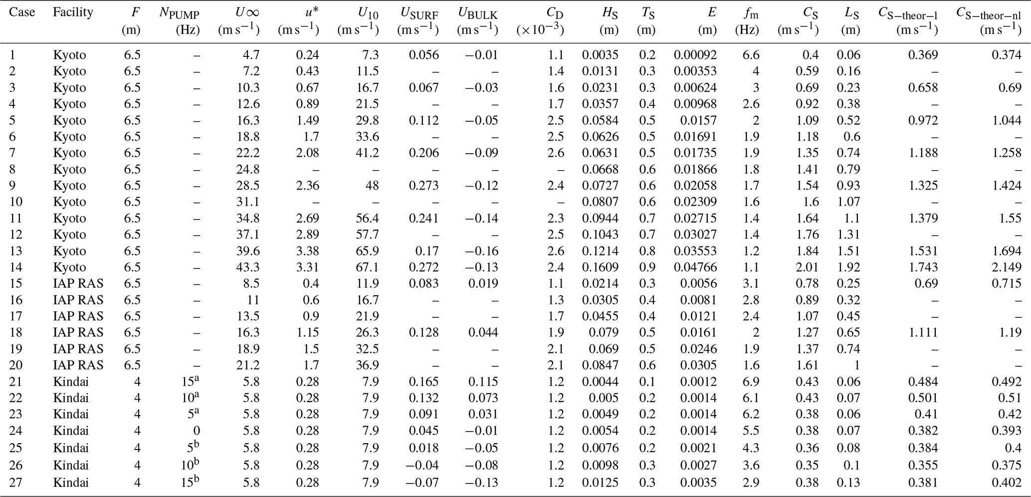
Superscripted a and b indicate the artificial following and opposing flows, respectively.
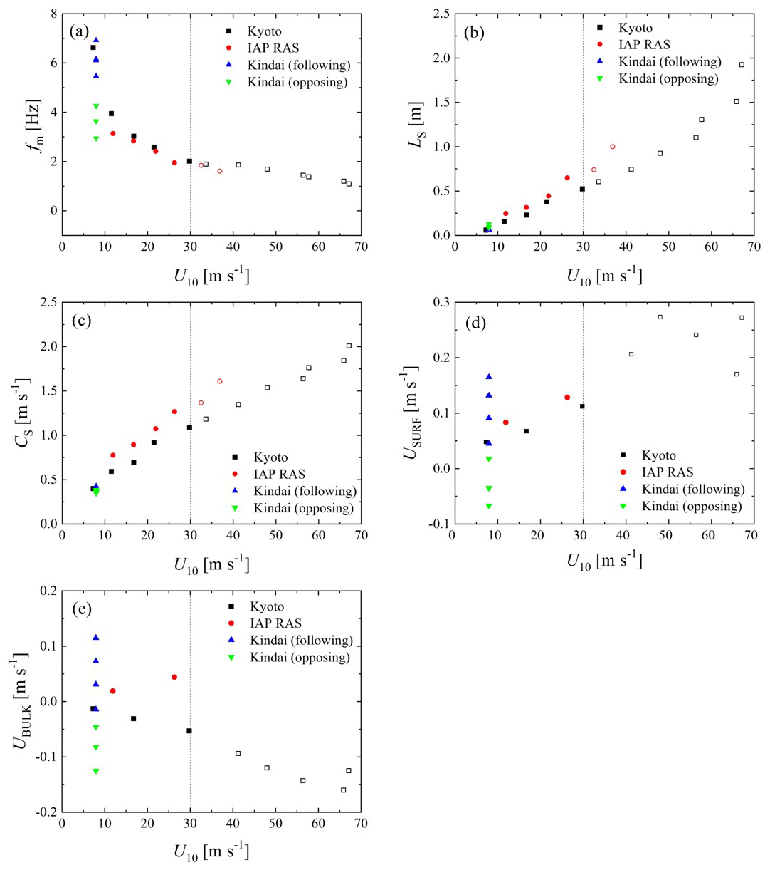
Figure 3Relationships between U10 and (a) significant frequency fm, (b) significant wavelength LS, (c) phase velocity CS, (d) surface velocity of water USURF, and (e) bulk velocity of water UBULK. Open symbols show the high-wind-speed cases.

Figure 4Dispersion relation between angular frequency ω and wavenumber k. Open symbols show the high-wind-speed cases. The curve shows the dispersion relation of the deepwater waves (ω2=gk).
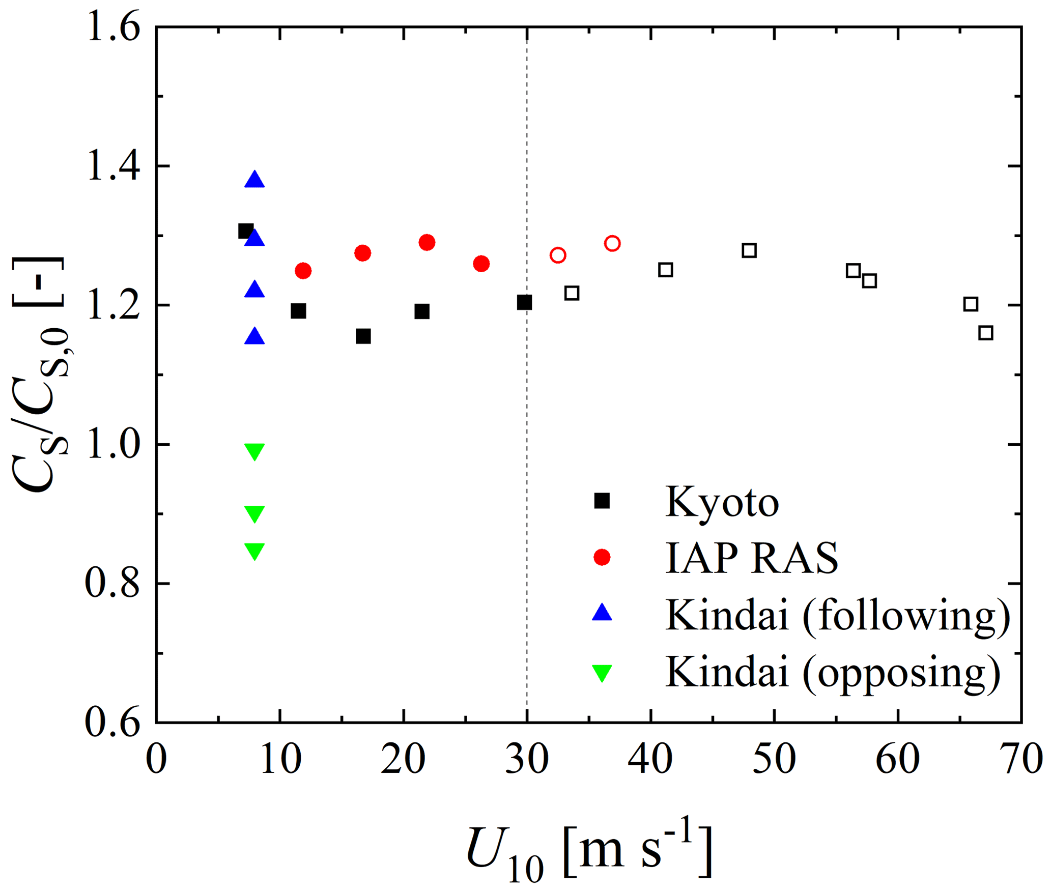
Figure 5Relationship between the free-stream wind speed and phase velocity CS. The CS is normalized by phase velocity CS,0 without the Doppler effect, estimated by the dispersion relation of the deepwater waves (). Open symbols show the high-wind-speed cases.
CS to the phase velocity CS,0 is estimated by the dispersion relation of deepwater waves () against the wind velocity. From the figure, the ratios at normal wind speeds assume a constant value (∼1.21 in Kyoto or ∼1.27 at IAP RAS). Moreover, the ratios at extremely high wind speeds take similar values of 1.23 and 1.28 for Kyoto and IAP RAS, respectively. This implies that the phase velocities at extremely high wind speeds are accelerated by the current just like those at normal wind speeds. However, the Kindai values are scattered and increase in the following cases and decrease in the opposing cases. It is clear that the artificial current accelerates (or decelerates) the phase velocity.
To interpret the relationship among the measured phase velocity CS, first phase velocity CS,0 estimated by the dispersion relation, and water velocity, two types of phase velocities were evaluated: the sum of CS,0 and the surface velocity of water USURF and the sum of CS,0 and the bulk velocity of water UBULK. Figure 6 shows the relationship of CS to (a) and (b) . In Fig. 6a, we can see that the Doppler shift is confirmed at normal wind speeds; i.e., significant waves are accelerated by the surface flow, and the real phase velocity can be represented as the sum of the velocity of the surface flow and the virtual phase velocity, which is estimated by the dispersion relation of the deepwater waves. At extremely high wind speeds over 30 m s−1, a similar Doppler shift is observed as under the conditions of normal wind speeds, as seen in Fig. 6a. Meanwhile, in Fig. 6b, although CS corresponds to at low phase velocities, CS assumes values larger than at high phase velocities. This suggests that the Doppler shift is an adequate model for representing the acceleration of wind waves by the current, not only for wind waves at normal wind speeds but also for those with intensive breaking at extremely high wind speeds. Moreover, the Doppler shift of wind waves occurs due to a very thin surface flow, as the correlation between CS and is higher than the correlation between CS and .
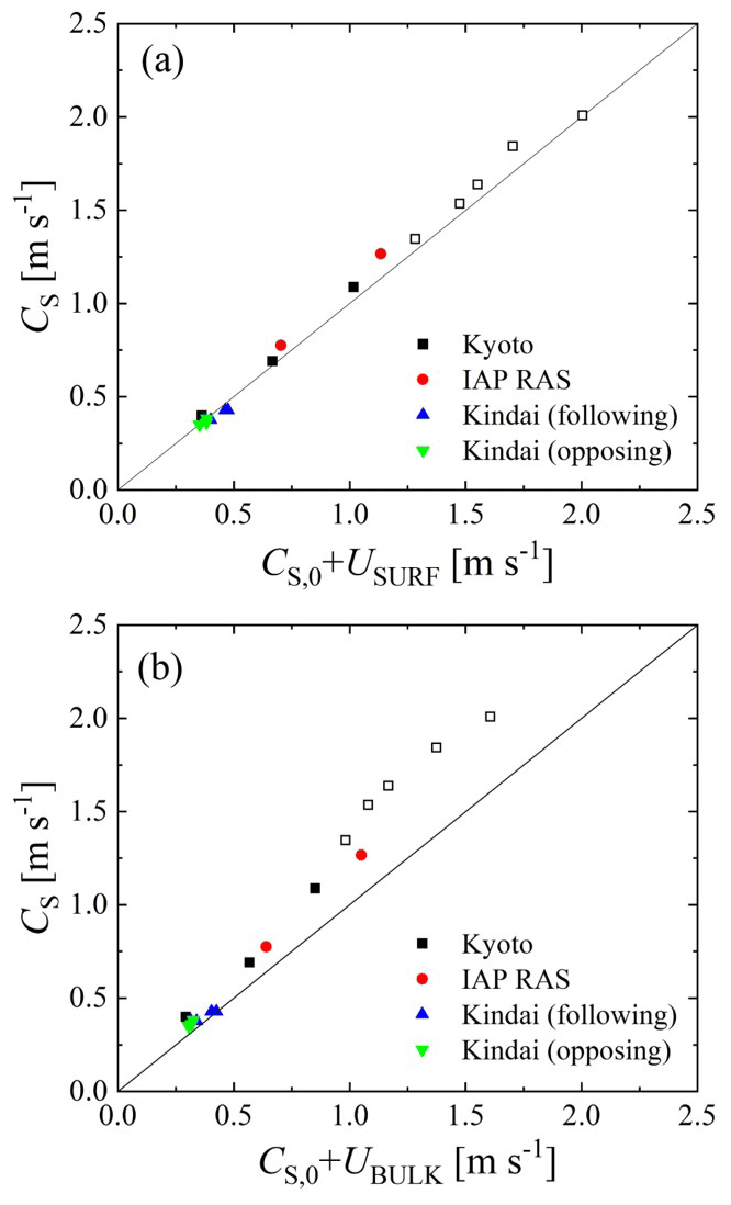
Figure 6Relationship between phase velocity CS and (a) the sum of CS,0 and the surface velocity of water USURF, as well as (b) the sum of CS,0 and the bulk velocity of water UBULK. Open symbols show the high-wind-speed cases.
3.2 The theoretical model of waves at the shear flow
The parameters of the observed Doppler shift can be explained more precisely within the theoretical model of capillary–gravity waves at the surface of the water flows with the velocity profiles prescribed by the experimental data, which are plotted in Fig. 2a–c. Because the dominant wind wave propagates along the wave and water flows, we will consider the 2D wave model in the 2D flow. This flow is described by the system of 2D Euler equations,
and the condition of non-compressibility,
with the kinematical,
and dynamical boundary conditions,
at the water surface. Here, u and w are the horizontal and vertical velocity components, p is the water pressure, x and z are the horizontal and upward vertical coordinates, g is the gravity acceleration, and ρ is the water density. The boundary condition at the bottom of the channel is . It should be noted that the water depth in almost all the experimental runs exceeded half of the wavelength of the dominant waves (see Table 1). In this case, the deepwater approximation is applicable for describing the surface waves, and the boundary condition of the wave field vanishing with the distance from the water surface can also be used.
Because the fluid motion under consideration is 2D, the stream function can be introduced as follows:
To derive the linear dispersion relation for the surface waves at the plane shear flow with the horizontal velocity profile Uw(z), we consider the solution to Eqs. (3) and (4) in terms of the stream function as the sum of the undisturbed state with steady shear flow and small-amplitude disturbances. Then, the stream function ψ and pressure p are as follows:
where ε≪1, and the water elevation value is also the order of ε, namely εη1(x,t).
In the linear approximation in ε, the system of Eqs. (3) and (4) and the boundary conditions of Eqs. (5) and (6) take the form
Excluding p1 with the use of the first equation of the system in Eq. (3) and eliminating η1 yields one boundary condition at the water surface for ψ1:
For the harmonic wave disturbance, where
substituting into Eqs. (10) and (11) yields the Rayleigh equation for the complex amplitude of the stream function disturbance,
with the following boundary condition:
Numerically solving the boundary layer problem for Eq. (13) with the boundary conditions in Eq. (14) enables one to obtain the dispersion relation ω(k) for surface waves at inhomogeneous shear flow. Note that because the phase velocity of the waves significantly exceeded the flow velocity in all experiments (compare Figs. 2 and 3), the Rayleigh equation did not have a singularity, and the calculated frequency and phase velocity of the wave were real values; i.e., the current was neutrally stable.
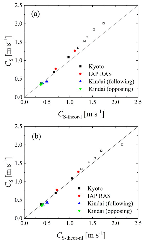
Figure 7The measured phase velocity CS versus theoretical prediction: (a) linear model and (b) nonlinear model.
The wave phase velocities were calculated for the parameters of those experiments that contained complete information about the course and characteristics of the waves, namely 1, 3, 5, 7, 9, 11, 13–15, 18, and 21–27 from Table 1. The results are presented in Fig. 7a as the measured phase velocity Cs versus calculated phase velocity . One can see that the model corresponds to the data substantially better than the model of linear potential waves at the homogeneous current UBULK (compare Fig. 6b). Considering the structure of the wave disturbances of the stream function, Ψ1(z) was found as the eigenfunction of the boundary problem in Eqs. (11) and (12). The profiles of Ψ1(z) are presented in Fig. 8. One can see that in all cases the functions Ψ1(z) are close to ekz at the background of the mean velocity profiles. Moreover, for experiment nos. 1, 3, 5, 15, and 21–27 (see Fig. 8a, b, c, i, and k), the wave field is concentrated near the surface at a distance less than the scale of the change in the mean flow, whereby the flow velocity is approximately equal to USURF. This explains the good correlation in these cases of the observed phase velocity with the phase velocity of waves at the homogeneous current USURF presented in Fig. 6a. At the same time, for experiment nos. 7, 9, 5, 11, 13, 14, and 18 (see Fig. 8d–h and j), the scale of the variability of the flow is significantly smaller than the scale of the wave field. Under these conditions, a significant difference between the phase velocity of the waves and that given by the linear dispersion relation can be due to the influence of nonlinearity.

Figure 8Vertical velocity profiles (points), their fitting (thin colored line), the eigenfunction of Eq. (8) with the boundary conditions in Eq. (9) (black solid curve), the function ekz (crosses), and the function e2 kz (dashed line). Panels (a)–(j) correspond to experiment nos. 1, 3, 5, 7, 9, 11, 13–15, and 18, respectively, and (k) corresponds to experiment nos. 21–27.
To estimate the nonlinear addition to the wave phase velocity, we used the results of the weakly nonlinear theory of surface waves for the current with a constant shear. Of course, the flow in the experiments of the present work does not have a constant shift, and this was considered when obtaining the linear dispersion relation. However, it should be taken into account that the contributions of the nth harmonic to the nonlinear dispersion relation are determined by wave fields in the n power, which have a scale that is n times smaller than the first harmonic. Additionally, the model of constant shear of the mean current velocity is already approximately applicable for the second harmonic (see Fig. 8).
We use the nonlinear dispersion relation for waves in the current with a constant shift in the deepwater approximation, which was obtained by Simmen and Saffman (1985):
Here, ω0 is the solution of the linear dispersion equation. Equation (15) is rewritten in the notation of this work and formulated in a reference frame in which the surface of the water has the velocity Uw(0). Note that the linear part of Eq. (15) coincides with Eq. (14). The results of solving Eq. (15) are presented in Fig. 7b similarly to Fig. 7a as the measured phase velocity CS versus calculated phase velocity; one can see their good agreement with each other. Thus, the wave frequency shift can be explained by two factors, including the Doppler shift at the mean flow and the nonlinear frequency shift, while the latter can also be interpreted in its physical nature as the wave frequency shift in the presence of its orbital velocities.
Recent studies have indicated a regime shift in the momentum, heat, and mass transfer across an intensive broken wave surface along with the amount of dispersed droplets and entrained bubbles at extremely high wind speeds over 30 m s−1 (e.g., Powell et al., 2003; Donelan et al., 2004; Takagaki et al., 2012, 2016; Troitskaya et al., 2012; Iwano et al., 2013; Krall and Jähne, 2014; Komori et al., 2018; Krall et al., 2019). Thus, there is the possibility of a similar regime shift in the Doppler shift of wind waves by the current at extremely high wind speeds. However, the present study reveals that such a Doppler shift is observed under the conditions of normal wind speeds. In this case, the weakly nonlinear approximation turns out to be applicable for describing the dispersion properties of not only small-amplitude waves but also nonlinear and even breaking waves. This implies that intensive wave breaking at extremely high wind speeds occurs with the saturation (or dumping) of the wave height rather than the wavelength. This evidence might be helpful in investigating and modeling wind-wave development at extremely high wind speeds.
The effects of the current on wind waves were investigated through laboratory experiments in three different wind-wave tanks with a pump at Kyoto University, Japan, Kindai University, Japan, and IAP RAS. The study investigated 27 cases with measurements of winds, waves, and currents at wind speeds ranging 7–67 m s−1. We observed that the wind waves do not follow the dispersion relation at either normal or extremely high wind speeds in the three tanks (Fig. 4) – excluding case 25, in which the artificial current experiment used the Kindai tank. In case 25, USURF is approximately zero (Fig. 3); thus, the Doppler shift does not occur. Then, using 18 datasets (Kyoto and IAP RAS tanks) (Fig. 5), we found that the ratio of is constant at both normal and extremely high wind speeds. Moreover, in the artificial current experiment in Kindai, we observed that the ratio varies (Fig. 5). The evidence from the three tank experiments implies that the same wave–current interaction occurs at normal and extremely high wind speeds.
To develop an adequate model for wave–current interaction at normal and extremely high wind speeds, we validated four models (Figs. 6 and 7). At normal wind speeds under 30 m s−1, the wave frequency, wavelength, and phase velocity of waves, as well as the surface velocity of the water depended on the wind speed (Fig. 3). However, the bulk velocity of the water showed a dependence on the tank type, i.e., a large tank with a submerged wind-wave flume (IAP RAS) or wind flume above a tank (general type of wind-wave tank) (Kyoto University) (Fig. 3). The effect of the Doppler shift was confirmed at normal wind speeds; i.e., significant waves were accelerated by the surface flow, and the phase velocity was represented as the sum of the surface velocity of water and the phase velocity, which is estimated by the dispersion relation of deepwater waves (Fig. 6). At extremely high wind speeds over 30 m s−1, a Doppler shift was observed similar to that under the conditions of normal wind speeds (Figs. 4 and 5). This suggests that the Doppler shift is an adequate model for representing the acceleration of wind waves by the current, not only for wind waves at normal wind speeds but also for those with intensive breaking at extremely high wind speeds. The data obtained by the artificial current experiments conducted at Kindai University were used to explain how the artificial current accelerates (or decelerates) significant waves. A weakly nonlinear model of surface waves at a shear flow was developed (Fig. 7). It was shown that it describes dispersion properties well not only for small-amplitude waves but also strongly nonlinear and even breaking waves, which are typical for extreme wind conditions, with speeds, U10, exceeding 30 m s−1.
It is important to estimate the phase velocity and wavelength of significant wind waves using the water-level fluctuation data. Here, we explain the method, called the cross-spectrum method. The water-level fluctuation η (x,t) at an arbitral location x and time t is shown as the equation
where ω is the angular frequency, A(ω) is the complex amplitude, k(ω) is the wavenumber of waves having ω, and Ω is the maximum angular frequency of the surface waves. Fη(ω) is the Fourier transformation of η (x, t) when the measurement time (tm) and Ω are sufficiently large. Using the inverse Fourier transformation of Fη(ω), η(x, t) is shown as
Comparing Eqs. (A1) and (A2), Fη(ω) is . Assuming that the wind waves change the shape little between two wave probes set upstream and downstream, we can set the upstream and downstream water-level fluctuations and , respectively, with Δx downstream from the first probe. The Fourier transformations Fη1(ω) and Fη2(ω) for η1(t) and η2(t), respectively, are shown as
Then, the power spectra Sη1η1(ω) and Sη2η2(ω) for η1(t) and η2(t), respectively, are shown as
Here, the superscript ∗ indicates the complex conjugate number. The cross-spectrum Cr(ω) for η1(t) and η2(t) is shown as
Using Euler's theorem, Eq. (A7) transforms to
The co-spectrum Co(ω) and quad spectrum Q(ω) are defined as the real and imaginary parts of Cr(ω), respectively, shown as Cr(ω) = Co(ω) + iQ(ω). Moreover, the phase θ(ω) is defined as θ(ω)= tan. Thus, θ(ω) can be calculated as
Generally, the velocity of the wind waves C is defined as
where L is the wavelength and T is the wave period. From Eqs. (A9) and (A10), C(ω) and L(ω) can be transformed to
When we estimate the phase θm(ωm) at the angular frequency of significant wind waves ωm (=2πfm), the phase velocity of significant wind waves CS (=C(ωm)) and significant wavelength LS (=L(ωm)) are calculated by
In the study, CS and LS are estimated by Eqs. (A13) and (A14) using the cross-spectrum method.
All analytical data used in this study are compiled in Table 1.
NT and NS planned the experiments, evaluated the data, and contributed equally to writing the paper excluding Sect. 3.2. YT planned the Russia experiment, provided the linear and nonlinear models, prepared figures in Sect. 3.2, and contributed to writing Sect. 3.2. CT prepared all figures excluding Sect. 3.2. NT performed the wind, current, and wave measurements in the Kyoto experiment. NT, NS, and CT performed the wind, current, and wave measurements in the Kindai experiment. AK and MV performed the wind, current, and wave measurements in the Russia experiment.
The authors declare that they have no conflict of interest.
This work was supported by the Ministry of Education, Culture, Sports, Science and Technology (Grant-in-Aid nos. 18H01284, 18K03953, and 19KK0087). This project was supported by the Japan Society for the Promotion of Science and the Russian Foundation for Basic Research (grant nos. 18-55-50005, 19-05-00249, and 20-05-00322) under the Japan–Russia Research Cooperative Program. The experiments of IAP RAS were partially supported by the RSF (project 19-17-00209). We thank Takumi Tsuji and Satoru Komori for their help in conducting the experiments and for useful discussions. The experiments of IAP RAS were performed at the Unique Scientific Facility “Complex of Large-Scale Geophysical Facilities” (http://www.ckp-rf.ru/usu/77738/, last access: 2 September 2020).
This research has been supported by the Ministry of Education, Culture, Sports, Science and Technology (grant nos. 18H01284, 18K03953, and 19KK0087), the Japan Society for the Promotion of Science, and the Russian Foundation for Basic Research (grant nos. 18-55-50005, 19-05-00249, and 20-05-00322).
This paper was edited by Judith Wolf and reviewed by two anonymous referees.
Dawe, J. T. and Thompson, L.: Effect of ocean surface currents on wind stress, heat flux, and wind power input to the ocean, Geophys. Res. Lett., 33, L09604, https://doi.org/10.1029/2006GL025784, 2006.
Donelan, M. A., Haus, B. K., Reul, N., Plant, W. J., Stiassnie, M., Graber, H. C., Brown, O. B., and Saltzman, E. S.: On the limiting aerodynamic roughness of the ocean in very strong winds, Geophys. Res. Lett., 31, L18306, https://doi.org/10.1029/2004GL019460, 2004.
Fan, Y., Ginis, I., and Hara, T.: The Effect of Wind–Wave–Current Interaction on Air–Sea Momentum Fluxes and Ocean Response in Tropical Cyclones, J. Phys. Oceanogr., 39, 1019–1034, 2009.
Holthuijsen, L. H., Powell, M. D., and Pietrzak, J. D.: Wind and waves in extreme hurricanes, J. Geophy. Res., 117, C09003, https://doi.org/10.1029/2012JC007983, 2012.
Iwano, K., Takagaki, N., Kurose, R., and Komori, S.: Mass transfer velocity across the breaking air-water interface at extremely high wind speeds, Tellus B, 65, 21341, https://doi.org/10.3402/tellusb.v65i0.21341, 2013.
Kara, A. B., Metzger, E. J., and Bourassa, M. A.: Ocean current and wave effects on wind stress drag coefficient over the global ocean, Geophys. Res. Lett., 34, L01604, https://doi.org/10.1029/2006GL027849, 2007.
Kawabe, M.: Variability of Kuroshio velocity assessed from the sea-level difference between Naze and Nishinoomote, J. Oceanogr. Soc. Jpn., 44, 293–304, 1988.
Kelly, K. A., Dickinson, S., McPhaden, M. J., and Johnson, G. C.: Ocean currents evident in satellite wind data, Geophys. Res. Lett., 28, 2469–2472, 2001.
Komori, S., Iwano, K., Takagaki, N., Onishi, R., Kurose, R., Takahashi, K., and Suzuki, N.: Laboratory measurements of heat transfer and drag coefficients at extremely high wind speeds, J. Phys. Oceanogr., 48, 959–974, https://doi.org/10.1175/JPO-D-17-0243.1, 2018.
Krall, K. E. and Jähne, B.: First laboratory study of air-sea gas exchange at hurricane wind speeds, Ocean Sci., 10, 257–265, https://doi.org/10.5194/os-10-257-2014, 2014.
Krall, K. E., Smith, A. W., Takagaki, N., and Jähne, B.: Air-sea gas exchange at wind speeds up to 85 m s−1, Ocean Sci., 15, 1783–1799, https://doi.org/10.5194/os-15-1783-2019, 2019.
Powell, M. D., Vickery, P. J., and Reinhold, T. A.: Reduced drag coefficient for high wind speeds in tropical cyclones, Nature, 422, 279–283, https://doi.org/10.1038/nature01481, 2003.
Shi, Q. and Bourassa, M. A.: Coupling Ocean Currents and Waves with Wind Stress over the Gulf Stream, Remote Sens., 11, 1476, https://doi.org/10.3390/rs11121476, 2019.
Simmen, J. A. and Saffman, P. G.: Steady deep-water waves on a linear shear current, Stud. Appl. Math., 73, 35–57, https://doi.org/10.1002/sapm198573135, 1985.
Takagaki, N., Komori, S., Suzuki, N., Iwano, K., Kuramoto, T., Shimada, S., Kurose, R., and Takahashi, K.: Strong correlation between the drag coefficient and the shape of the wind sea spectrum over a broad range of wind speeds, Geophys. Res. Lett., 39, L23604, https://doi.org/10.1029/2012GL053988, 2012:
Takagaki, N., Komori, S., Suzuki, N., Iwano, K., and Kurose, R.: Mechanism of drag coefficient saturation at strong wind speeds, Geophys. Res. Lett., 43, 9829–9835, https://doi.org/10.1002/2016GL070666, 2016.
Takagaki, N., Komori, S., Ishida, M., Iwano, K., Kurose, R., and Suzuki, N.: Loop-type wave-generation method for generating wind waves under long-fetch conditions, J. Atmos. Ocean. Tech., 34, 2129–2139, https://doi.org/10.1175/JTECH-D-17-0043.1, 2017.
Takagaki, N., Suzuki, N., Takahata, S., and Kumamaru, H.: Effects of air-side freestream turbulence on development of wind waves, Exp. Fluids, 61, 136, https://doi.org/10.1007/s00348-020-02977-9, 2020.
Troitskaya, Y. I., Sergeev, D. A., Kandaurov, A. A., Baidakov, G. A., Vdovin, M. A., and Kazakov, V. I.: Laboratory and theoretical modeling of air-sea momentum transfer under severe wind conditions, J. Geophys. Res., 117, C00J21, https://doi.org/10.1029/2011JC007778, 2012.
Troitskaya, Y. I., Kandaurov, A., Ermakova, O., Kozlov, D., Sergeev, D., and Zilitinkevich, S.: Bag-breakup fragmentation as the dominant mechanism of sea-spray production in high winds, Sci. Rep., 7, 1614, https://doi.org/10.1038/s41598-017-01673-9, 2017.
Troitskaya, Y. I., Kandaurov, A., Ermakova, O., Kozlov, D., Sergeev, D., and Zilitinkevich, S.: Bag-breakup spume droplet generation mechanism at hurricane wind, Part I. Spray generation function, J. Phys. Oceanogr., 48, 2167–2188, https://doi.org/10.1175/JPO-D-17-0104.1, 2018a.
Troitskaya, Y. I., Druzhinin, O., Kozlov, D., and Zilitinkevich, S.: Bag-breakup spume droplet generation mechanism at hurricane wind, Part II. Contribution to momentum and enthalpy transfer, J. Phys. Oceanogr., 48, 2189–2207, https://doi.org/10.1175/JPO-D-17-0105.1, 2018b.
Troitskaya, Y., Sergeev, D., Vdovin, M., Kandaurov, A., Ermakova, O., and Takagaki, N.: Laboratory study of the effect of surface waves on heat and momentum transfer at strong winds, J. Geophys. Res.-Ocean, 125, e2020JC016276, https://doi.org/10.1029/2020JC016276, 2020.