the Creative Commons Attribution 4.0 License.
the Creative Commons Attribution 4.0 License.
 | 11 Feb 2019
Could the two anticyclonic eddies during winter 2003/2004 be reproduced and predicted in the northern South China Sea?
Dazhi Xu
Wei Zhuang
Great progress has been made in understanding the mesoscale eddies and their role on the large-scale structure and circulation of the oceans. However, many questions still remain to be resolved, especially with regard to the reproductivity and predictability of mesoscale eddies. In this study, the reproductivity and predictability of mesoscale eddies in the northern South China Sea (NSCS), a region with strong eddy activity, are investigated with a focus on two typical anticyclonic eddies (AE1 and AE2) based on a HYCOM–EnOI assimilated system. The comparisons of assimilated results and observations suggest that generation, evolution, and propagation paths of AE1 and AE2 can be well reproduced and forecasted when the observed amplitude is >8 cm (or the advective nonlinearity parameter U∕c is >2), although their forcing mechanisms are quite different. However, when their amplitudes are less than 8 cm, the generation and decay of these two mesoscale eddies cannot be well reproduced and predicted by the system. This result suggests, in addition to dynamical mechanisms, that the spatial resolution of assimilation observation data and numerical models must be taken into account in reproducing and predicting mesoscale eddies in the NSCS.
- Article
(12486 KB) - Full-text XML
- BibTeX
- EndNote


Equivalent to the synoptic variability of the atmosphere, ocean mesoscale eddies are often described as the “weather” of the ocean, with typical spatial scales of ∼100 km and timescales of a month (Wang et al., 1996; Liu et al., 2001; Chelton et al., 2011). The mesoscale eddy is characterized by temperature and salinity anomalies with associated flow anomalies, exhibiting different properties to their surroundings, thus allowing them to control the strength of mean currents and to transport heat, salt, and biogeochemical tracers around the ocean. The motion of mesoscale eddies would be a straight line if eddies freely propagate in the open ocean. However, most eddies may have interactions with topography, strong currents (western boundary current), and other eddies during their lifetime. The motion of an eddy will be modified and even split when approaching an island (Yang et al., 2017). It is also recognized that the western boundary is where eddies disappear (Zhai et al., 2010). The dynamical processes, such as splitting and/or merging of eddies, can also result in termination and/or genesis of eddies in the open ocean (Li et al., 2016). Thus, the dynamical processes mean that the prediction of eddy motion is a challenge for ocean simulation. Although the beauty and complexity, temporal and spatial variability, eddy energy and tracking, and the effects on atmosphere of these mesoscale features can be seen today by viewing high-resolution satellite images or numerical model simulations (Yang et al., 2000; Fu et al., 2010; Morrow and Le Traon, 2012; Frenger et al., 2013), the operational forecasts of the mesoscale eddy still pose a big challenge because of its complicated dynamical mechanisms and high nonlinearity (Woodham et al., 2015; Treguier et al., 2017; Vos et al., 2018). A recent example is the explosion of the Deepwater Horizon drilling platform in the northern Gulf of Mexico in 2010 where an accurate prediction of the position and propagation of the Loop Current eddy was essential in determining if the spilled oil would be advected to the Atlantic Ocean or still remain within the Gulf (Treguier et al., 2017).
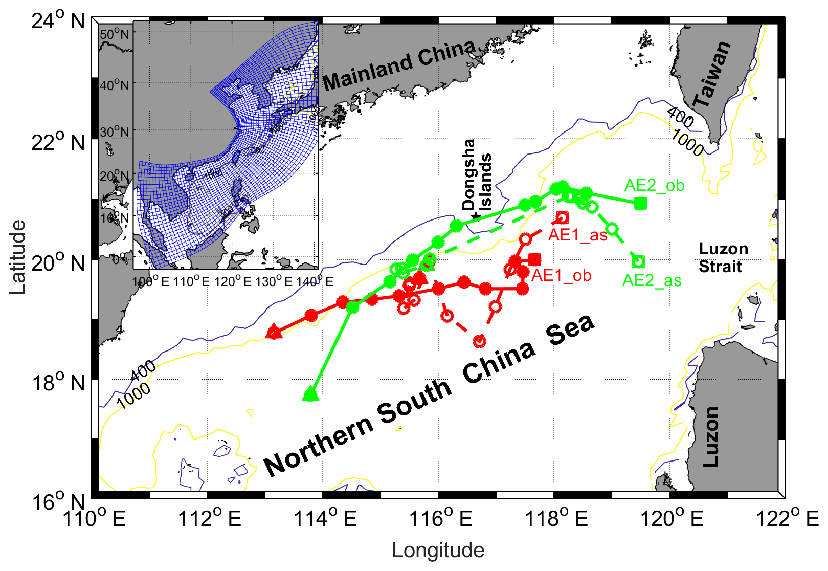
Figure 1Bathymetry of the northern South China Sea. The blue and yellow contour lines are the isolines of 400 and 1000 m, respectively. The solid black cross indicates Dongsha Islands. The migration path of AE1 and AE2 in the NSCS during December 2003–April 2004 are shown. Solid (hollow) red dots and solid (dash) lines indicate weekly passing position and migration path of observation (assimilation) AE1. Solid (hollow) green dots and solid (dash) lines indicated weekly passing position and migration path of observation (assimilation) AE2. The squares and triangles denote start and end positions, respectively. The model domain of CSCS (the inset panel), the curvilinear orthogonal model grid with 1∕8– horizontal resolution (147×430) is denoted by the blue grid (at intervals of 10 grid cells here).
Similar to the Gulf of Mexico, the South China Sea (SCS) is also a large semi-closed marginal sea, in the northwest Pacific, connecting to the western Pacific through the Luzon Strait (LS; Fig. 1). Forced by seasonal monsoon winds, the intrusion of the Kuroshio Current (KC), Rossby waves, and the complex topography, SCS and especially the northern SCS (NSCS) exhibits significant mesoscale eddy activity (Fig. 2). Many studies have tried to investigate mesoscale eddies in the NSCS (Wang et al., 2003, 2008; Jia et al., 2005). Based on the potential vorticity conservation equation and in situ survey data, Yuan and Wang (1986) pointed out that the bottom topography forcing might be the primary factor for the formation of anticyclonic eddies northeast of Dongsha Islands (DIs). Using survey CTD data in September 1994, Li et al. (1998) recorded evidence of anticyclonic eddies in the NSCS and suggested these anticyclonic eddies are probably shed from the KC. Investigations by Wu et al. (2007) showed that westward-propagating eddies in the NSCS originate near the LS rather than coming from the western Pacific. Based on the altimeter, trajectory of drift, and hydrological observation data, Wang et al. (2008) studied the evolution and migration of two anticyclonic eddies in the NSCS during winter of 2003/2004. As they described it, the AE1 generated by interaction of the unstable rotating fluid with the sharp topography of DIs firstly appeared near DIs on the 10 December 2003 (see Fig. 3). Then it began to move southwestward with its amplitude decreasing gradually. During the movement of AE1, another anticyclonic eddy (AE2) was shed and developed from the loop current of Kuroshio near the LS on the 14 January 2004. The amplitude of AE2 was then increased when it propagated southwestward (Fig. 3d–f). About 5 weeks later, AE2 reached its maximum in amplitude and then lasted around 3 weeks in its mature state. During its decay phase, AE2 moved southwestward quickly with its amplitude decreasing, and finally disappeared at the location of 18∘ N, 114∘ E on the 7 April 2004. Meanwhile, AE1 continued moving to southwest and eventually disappeared the southeast of Hainan. In addition to physical characteristics, the phytoplankton community at these two eddies have also been studied by Huang et al. (2010). These studies improved our understanding of the activities of mesoscale eddies and their possible dynamical mechanisms in the NSCS.
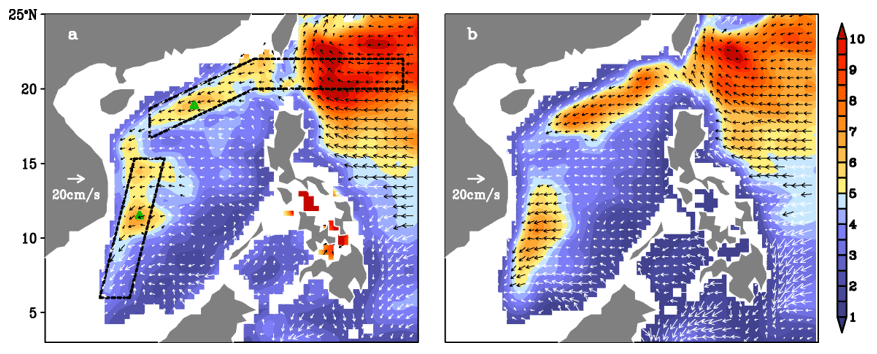
Figure 2Annual mean standard deviation of sea level mesoscale signals (color shading, unit: cm) and propagation velocities of the signals (vectors) derived from (a) altimeter observations and (b) OFES (Ocean General Circulation Model for the Earth Simulator) simulations. Cited from Zhuang et al. (2010).
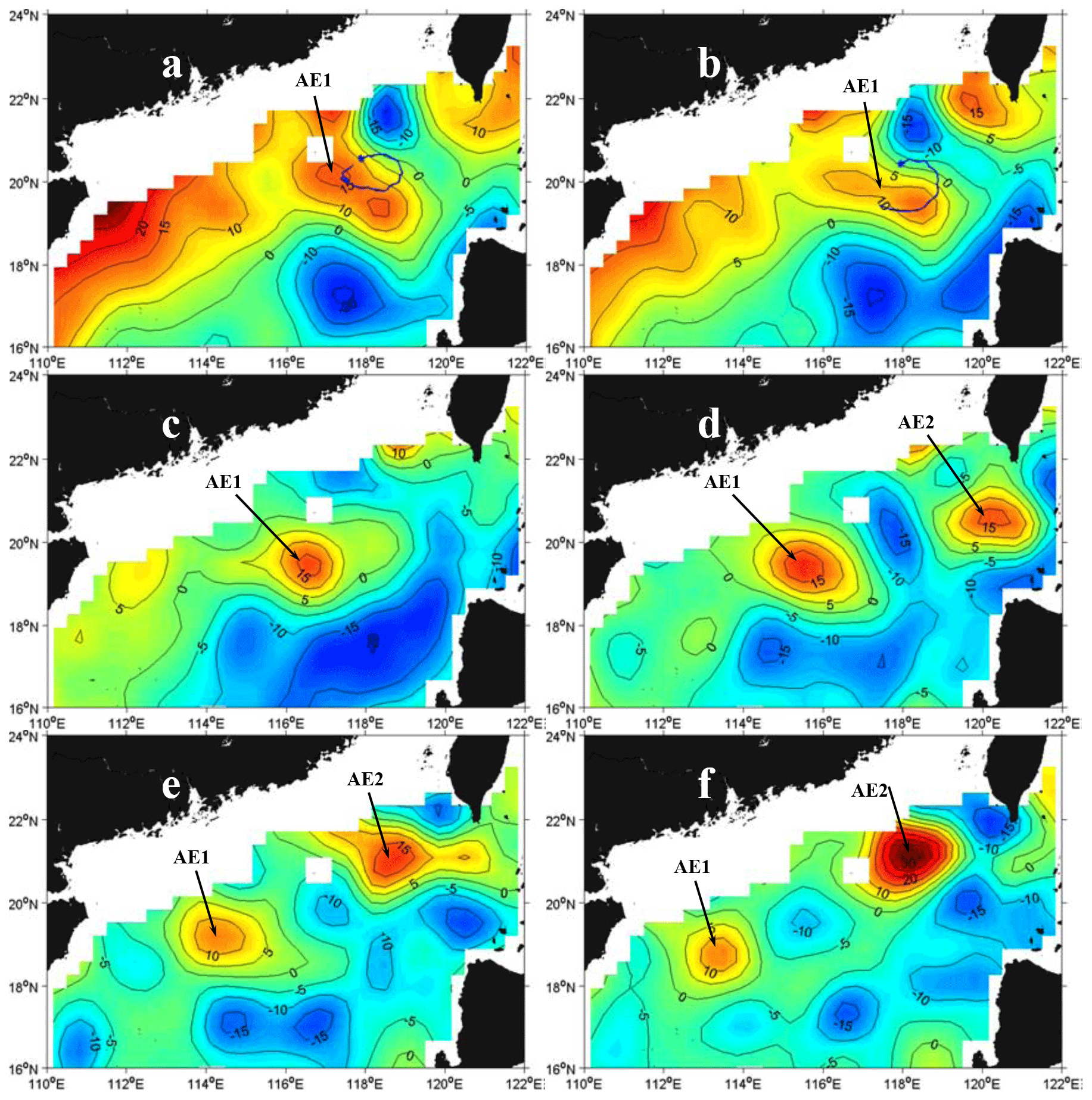
Figure 3Snapshots of sea level anomaly (SLA) from satellite remote sensing datasets. Buoy 22918 trajectory (blue lines, blue asterisk represents the initial position of buoy, as in Fig. 4) (a) from 4 to 15 December 2003 superposed on SLA field on 10 December 2003; (b) from 16 to 23 December 2003 superposed on SLA field on 17 December 2003; SLA field on (c) 7 January 2004, (d) 21 January 2004, (e) 4 February 2004, and (f) 18 February 2004. Cited from From Wang et al. (2008).
Despite the activities and possible dynamical mechanisms of mesoscale eddies in the NSCS having received much attention in past decades, studies on the reproductivity and predictability of mesoscale eddies in the NSCS are still rare. As mentioned above, mesoscale eddies are not only related to complicated dynamical mechanisms but also involve strong nonlinear processes (Oey et al., 2005); they are not a deterministic response to atmospheric forcing. The quality of mesoscale eddy forecasting will depend primarily on the quality of the initial conditions. Ocean data assimilation, which combines observations with the numerical model, can provide more realistic initial conditions and thus is essential for the prediction of mesoscale eddies. As shown by previous studies, after assimilating altimeter data into ocean models, the ocean currents in the southern SCS (Xiao et al., 2006) and the realism of the three largest eddies in the SCS during Typhoon Rammasun (Xie et al., 2018) have been improved. Furthermore, some studies show that the ocean model including tides or assimilated altimeter data with reasonable mean dynamic topography (MDT) can provide more realistic initial conditions (Xie et al., 2011; Xu et al., 2012). The above studies show that the mesoscale eddies in the SCS are reproducible, but the predictability of mesoscale eddies is rare. In this study, we assessed the reproduction and predictability of two typical anticyclonic eddies (Wang et al., 2008) chosen as representing different generation mechanisms and surviving long enough to be useful, with a focus on their generation, evolution, and decay processes by a series of numerical experiments based on a Chinese shelf/coastal seas assimilation system (CSCAS; Li, 2009; Li et al., 2010; Zhu, 2011) along with the observation data from surface drifter trajectories and satellite remote sensing.
2.1 Datasets
In this study, altimetric data in 2003–2004 was selected, including along-track sea level anomaly (SLA), totaling 29 passes (about 9300 points) over the domain of the Chinese shelf/coastal seas (CSCS). Considering the noise of SLA measurement in the shallow seas, data for the shallow areas with depth <400 m was excluded. In order to verify the merged SLA based on Jason-1, TOPEX/Poseidon, ERS-2, and ENVISAT (Ducet et al., 2000) provided by Archiving, Validation and Interpretation of Satellites Oceanographic data (AVISO) at Collecte Localisation Satellites (CLS, http://www.aviso.oceanobs.com/en/data/products/sea-surface-height-products, last access: June 2018), the resolution and weekly average are used. In addition, because the SLA present only the anomalies relative to a temporal mean sea level field, a new mean dynamic topography (nMDT), which has been corrected using an iterative method by Xu et al. (2012), was used to calculate the realistic sea level in this study.
In addition to SLA datasets, the daily optimum interpolation sea surface temperature (OISST) from the National Oceanic and Atmospheric Administration's (NOAA) National Climatic Data Center (ftp://eclipse.ncdc.noaa.gov/pub/OI-daily-v2/NetCDF/, last access: 31 January 2019) – which was merged by an optimum interpolation method (Reynolds et al., 2007) based on the infrared sea surface temperature (SST) collected by the Advanced Very High Resolution Radiometer sensors on the NOAA Polar Orbiting Environmental Satellite and SST from the Advanced Microwave Scanning Radiometer for the Earth Observing System – are also used. The daily OISST biases were fixed using in situ data from ships and buoys. The dataset between 2003 and 2004 was used in this study with a spatial resolution of . In addition, the surface drifting buoy data from the World Ocean Circulation Experiment (WOCE, ftp://ftp.aoml.noaa.gov/pub/phod/buoydata/, last access: 31 January 2019) are also used. Three drifters were designed to drift at the surface within the upper 15 m and tracked by the ARGOS satellite system. Positions of the drifters were smoothed using a Gaussian-filter timescale of 24 h to eliminate tidal and inertial currents, and were subsampled at 6 h intervals (Hamilton et al., 1999).
2.2 Method to identify the mesoscale eddies
Similar to the standard of Cheng et al. (2005) and Chelton et al. (2011), we identify the mesoscale eddies in this study as follows: (1) there must be a closed contour on the merged SLA; (2) there must be one maximum or minimum inside the area of the closed contour for anticyclonic or cyclonic eddies; (3) the difference between the extremum and the outermost closed SLA contour, i.e., the amplitude of the mesoscale eddy, must be greater than 2 cm; and (4) the spatial scale of the eddy should be 45–500 km. In addition, the amplitude (A) of an eddy is defined here to be the magnitude of the difference between the estimated basal height of the eddy boundary and the extremum value of sea surface height (SSH) within the eddy interior: .
2.3 Ocean model
Here we used a three-dimensional hybrid coordinate ocean model (HYCOM; Halliwell et al., 1998, 2000; Bleck, 2002; Halliwell, 2004; Chassignet et al., 2007) to provide a dynamical interpolator of observation data in the assimilation system. HYCOM is a primitive equation general ocean circulation model with vertical coordinates: isopycnic coordinate in the open stratified ocean, the geopotential (or z) coordinate in the weakly stratified upper ocean, and the terrain following sigma coordinate in shallow, coastal regions.
In this study, HYCOM was implemented in the CSCS with a horizontal resolution of , and in the remaining regions with ; the model domain is from 0 to 53∘ N and from 99 to 143∘ E, and the detailed model domain and grid can be referred to in the inset panel of Fig. 1. The vertical water column from the sea surface to the bottom was divided into 22 levels. The K-profile parameterization (KPP; Large et al., 1994), which has proved to be an efficient mixing parameterization in many oceanic circulation models, was used here. The bathymetry data of the model domain were taken from the 2 min Gridded Global Relief Data (ETOPO2).
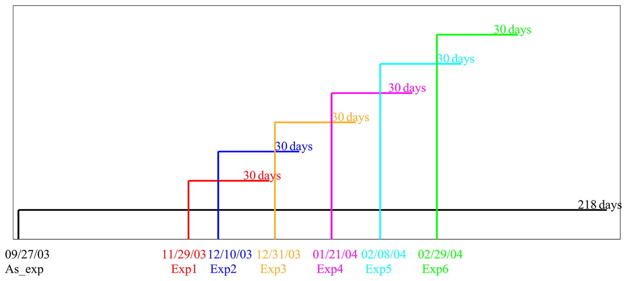
Figure 4The settings of assimilation and six forecast experiments, including the start dates and durations.
To adjust the model dynamics and achieve a perpetually repeating seasonal cycle before applying the interannual atmospheric forcing, the model was initialized with climatological temperature and salinity from the World Ocean Atlas 2001 (WOA01; Boyer et al., 2005) and was driven by the Comprehensive Ocean-Atmosphere Data Set (COADS; Woodruff et al., 1987) in the spin-up stage. After integrating 10 model years with climatological forcing, the model was forced by the European Centre for Medium-Range Weather Forecasts (ECMWF) 6-hourly reanalysis dataset (Uppala et al., 2005) from 1997 to 2003. The wind velocity (10 m) components were converted to stresses using a stability dependent drag coefficient from Kara et al. (2002). Thermal forcing included air temperature, relative humidity, and radiation (shortwave and longwave) fluxes. Precipitation was also used as a surface forcing from Legates and Willmott (1990). Surface latent and sensible heat fluxes were calculated using bulk formulae (Han, 1984). Monthly river runoff was parameterized as a surface precipitation flux in the East China Sea (ECS), the SCS and, LS from the river discharge stations of the Global Runoff Data Centre (GRDC; http://www.bafg.de, last access: 31 January 2019), and scaled as in Dai et al. (2002). Temperature, salinity, and currents at the open boundaries were provided by an India-Pacific domain HYCOM simulation at spatial resolution (Yan et al., 2007). Surface temperature and salinity were relaxed to climatology on a timescale of 100 days. Both two-dimensional barotropic fields such as SSH and barotropic velocities, and three-dimensional baroclinic fields such as currents, temperature, salinity, and density were stored daily.
2.4 The assimilation scheme
The ensemble optimal interpolation scheme (EnOI; Oke et al., 2002), which is regarded as a simplified implementation of the ensemble Kalman filter (EnKF), aims at alleviating the computational burden of the EnKF by using stationary ensembles to propagate the observed information to the model space. The data assimilation schemes can be briefly written as (Oke et al., 2010):
where ψ is the model state vectors including model temperature, layer thickness, and velocity; Superscripts a and b denote analysis and background, respectively; d is the measurement vector that consists of SST and SLA observations; K is the gain matrix; and H is the measurement operator that transforms the model state to observation space. P is the background error covariance and R is the measurement error covariance. In EnOI, Eq. (2) can be expressed as:
where α is a scalar that can tune the magnitude of the analysis increment; σ is a correlation function for localization; and Pb is the background error covariance that can be estimated by
In Eq. (4), n is the ensemble size, A′ is the anomaly of the ensemble matrix, ( is the ensemble members, N is the dimension of the model state, usually representing the model variability at certain scales by using a long-term model run or spin-up run. A more detailed description and evaluation of the CSCAS are in Li et al. (2010) and Xu et al. (2012).
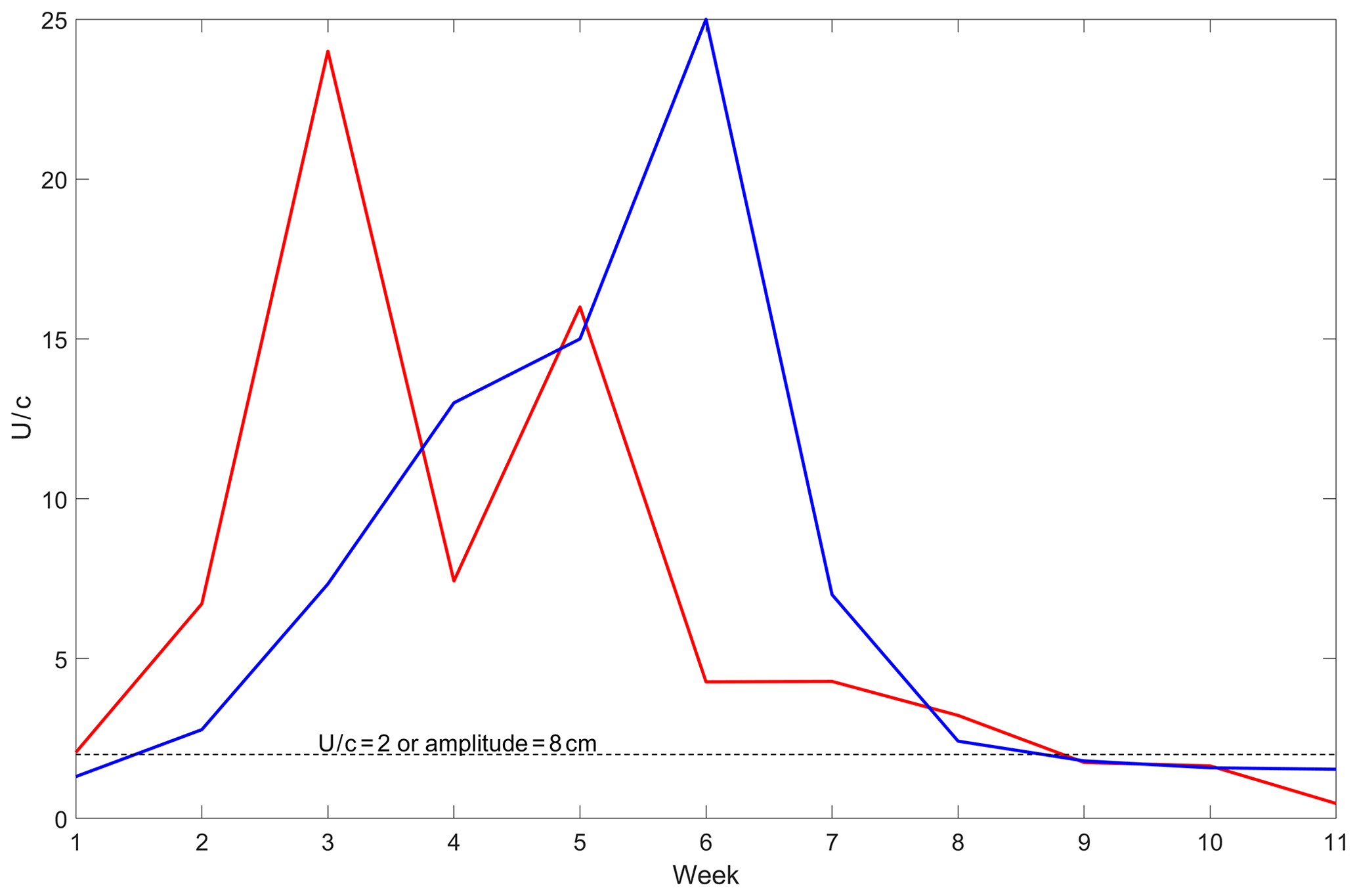
Figure 5The advective nonlinearity parameter U∕c (ANP). The thick red (blue) curve indicates the ANP of the observations (As_exp experiment) of AE2, the dashed line indicates the value of eddy amplitude at 8 cm or the ANP greater than 2.
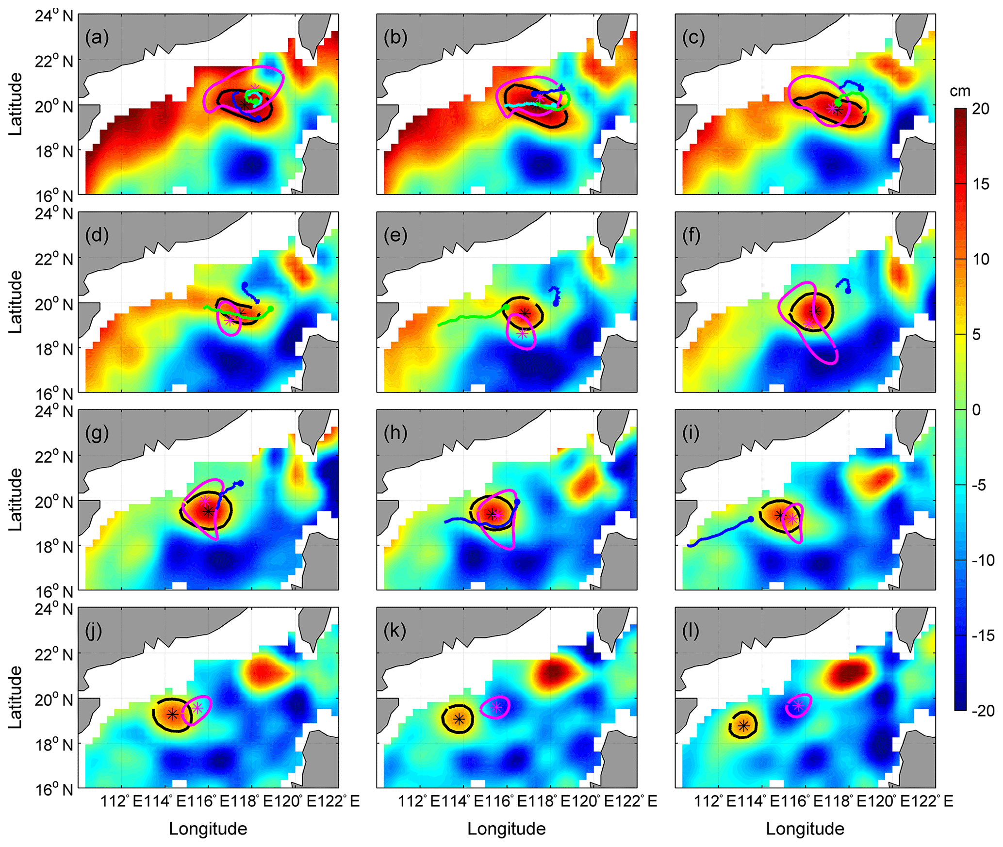
Figure 6Comparisons of AE1 derived from weekly SLA of assimilation results and observation from satellite remote sensing during the period of December 2003–February 2004. Background color is SLA; “*” symbols mark and closed lines indicate the center position and the outermost closed isoline of AE1, respectively; the black line is from satellite observation SLA and the pink line is from assimilation SLA. The cyan, green, and blue solid circular lines indicate the start positions and trajectories of numbers 22517, 22918, and 22610 drifter buoys, respectively; (a–l) is SLA on the 3 December 2003–18 February 2004, respectively; unit: cm.
3.1 The reproduction of anticyclonic eddies AE1 and AE2 in the NSCS
In order to investigate whether the evolution and migration features of these two eddies can be reproduced by the CSCAS or not, we firstly set up an assimilation experiment named As_exp (see Fig. 4, black line) for AE1 and AE2. In this experiment, the observed SST and SLA are both assimilated into CSCAS every 3 days. To meet dynamic adjustment, the first assimilation was performed on the 27 September 2003, 2 months prior to the generation of AE1.
Based on the As_exp experiment output, we use the observation SLA to evaluate the uncertainty of CSCAS in the research area. In this study, we calculated the weekly mean root mean square error (RMSE) of the As_exp and control experiment outputs and observations for SLA. As the results indicate, the RMSE for the As_exp is between 6 and 14 cm, while RMSE for the control is between 10 and 18 cm. This result suggested that data assimilation effectively improved the SLA field and had a beneficial impact on model results in this area.
In addition, we also use the advective nonlinearity parameter U∕c (ANP; Chelton et al., 2011; Li et al., 2014, 2015, 2016; Wang et al., 2015) as a criterion to estimate the eddy forecast ability of the CSCAS. As Fig. 5 shows, when the ANP is greater than 2 (that is the amplitude greater than 8 cm in our runs) AE2 can be reproduced by the CSCAS.
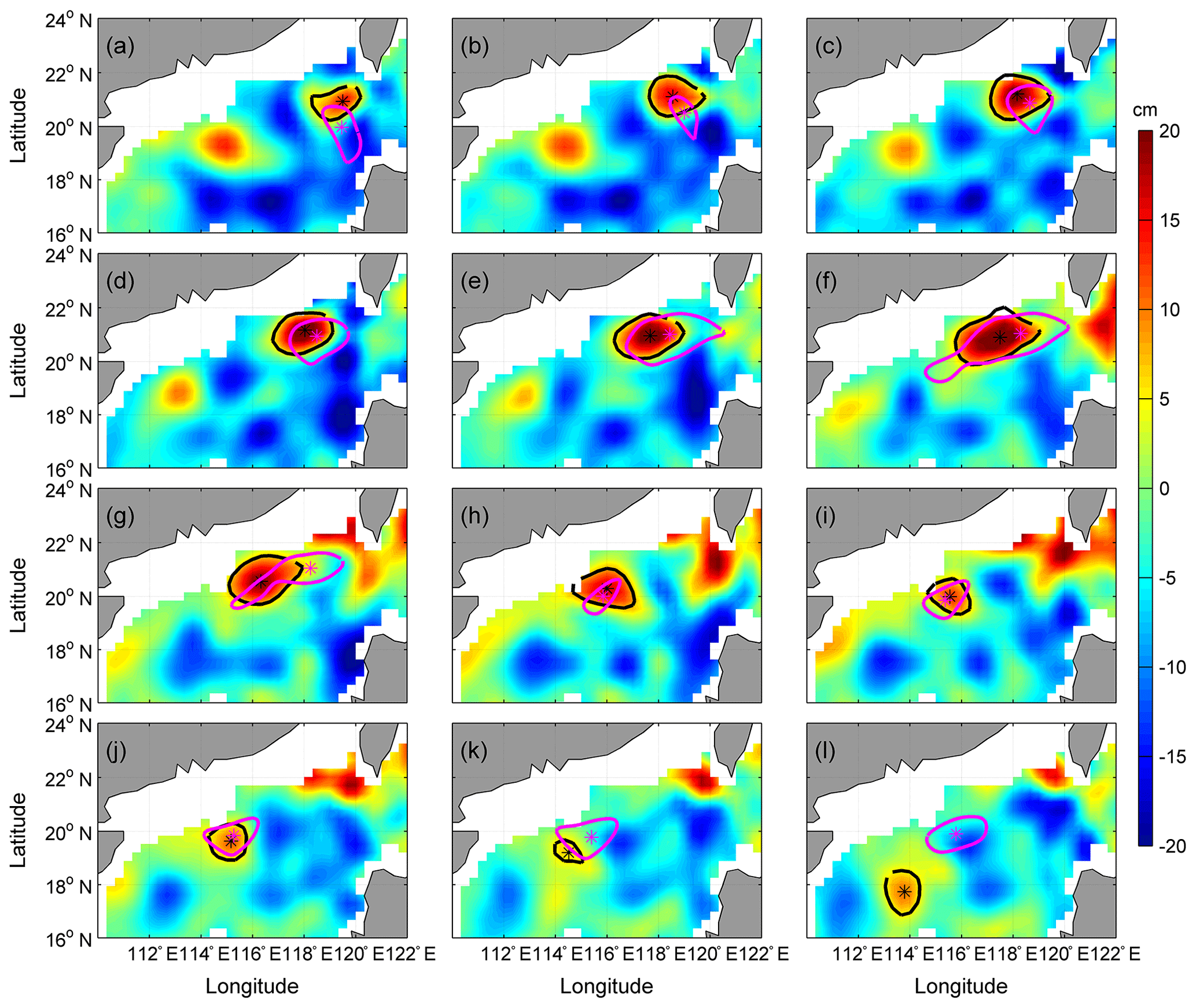
Figure 7The same as Fig. 6, but for AE2; the corresponding period is 28 January 2003–14 April 2004.
Table 1The amplitude of AE1 and AE2 derived from observation SLA and the assimilation SLA, and distance of eddy centers between the observation SLAs and assimilation SLAs.
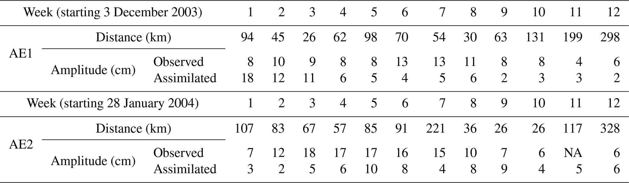
Besides, we also use the independent evaluation. Fig. 6 compares the assimilating results of AE1 with observations from both the satellite remote sensing and drifter buoys trajectories of numbers 22517, 22918, and 22610 between 3 December 2003 and 18 February 2004. From Fig. 6 and Table 1, we can see that the generation and movement of AE1 can be well reproduced by the CSCAS; the pink curves (assimilation) match well with those of the black (satellite observations) and dotted lines (the trajectories of drifter buoys). In addition, the spatial pattern of AE1 can also be well revealed by the CSCAS: the meridional and zonal radii of AE1 detected by the assimilation are 163 and 93 km, respectively, which are almost equal to that of observations (148 and 79 km). The migration path of AE1 can also be well reproduced by the CSCAS (see Fig. 6, black and pink lines) until its amplitude decays to less than 8 cm. In addition to AE1, the generation and evolution of AE2 are also evaluated. As shown Fig. 7, the evolution and propagation pathway of AE2 (Fig. 7b–j), e.g., moving firstly northwestward and then southwestward, can generally be reproduced by the CSCAS, although its initial location shows a slight southward bias in the simulation (Fig. 7a). Similar to the results of AE1, discrepancies between model and observations become larger again during the decay phase of AE2.
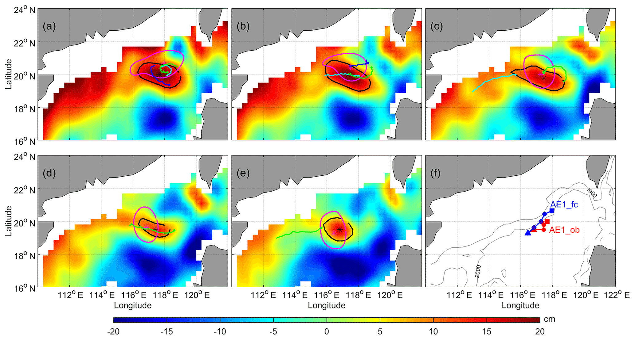
Figure 8Comparison of AE1 of Exp1 to observation, and trajectories of drifter buoys during the 29 November 2003 and the 29 December 2004. The cyan, green, and blue solid dots and lines indicate the start positions and trajectories of numbers 22917, 22918, and 22610 drift buoys during the corresponding period, respectively. Where, the red (blue) dotted line in (f) is the path of AE1 derived from observation (forecast) SLA during the experiment period, the square (triangle) represents the start (end) position.
In general, the comparison of assimilation SLA with that of satellite observation and the trajectories of drifter buoys suggested that the generation, development, and the propagation of AE1 and AE2 can be reproduced by the CSCAS when their observed amplitude is greater than 8 cm (or the ANP greater than 2). However, when their amplitudes are relatively small, less than 8 cm, the features of these two mesoscale eddies are not well reproduced by the CSCAS. This may be related to the value of parameter α, the localization length scale, or insufficient spatial resolution of assimilated SSH or the numerical model (Counillon and Bertino, 2009).
3.2 The predictability of these anticyclonic eddies in the NSCS
Since the generation, development, and the propagation of AE1 and AE2 can be well reproduced by the CSCAS when their amplitude >8 cm (or the ANP greater than 2), as mentioned above, in this section we further use the CSCAS to investigate the predictability of these two eddies. According to the generation, evolution, and migration of these two eddies, we designed six forecast experiments, hereafter referred to as Exp1 to Exp6 (see Fig. 4) to investigate their predictability. The model's initial state prior to each of the six forecast experiments is constrained by assimilating satellite SLA and SST before. Based on the initial state, each experiment is run forward 30 days with the forcing of 6-hourly wind, surface heat flux, monthly mean river runoff, etc. The first experiment, named Exp1, is applied on the 29 November 2003, which tends to study whether the generation of AE1 can be forecasted or not. Exp2 is implemented on the 10 December 2003 and is used to study whether the development and the migration of AE1 can be forecasted. Exp3 is run based on the initial state on the 31 December 2003 and used to show whether the generation of AE2 and the continued migration of AE1 can be forecasted. In order to investigate whether the continued evolution of AE1 and AE2 can be forecasted, Exp4 is applied on the 21 January 2004. Exp5 is set up to reveal whether the attenuation of AE1 and the evolution of AE2 can be forecasted, while Exp6, which is applied on the 29 February 2004, was designed to find out whether the disappearance of AE1 and AE2 can be forecasted.
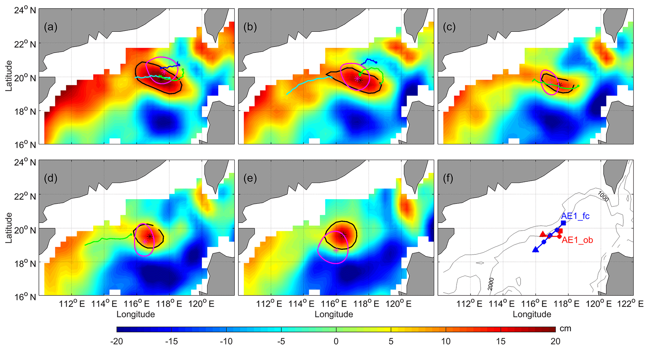
Figure 9Same as Fig. 8, but for Exp2; the experiment period is the 10 December 2003 to the 9 January 2004.
Table 2The amplitude of AE1 and AE2 derived from observation SLA and the six forecast SLA, and distance of eddy centers between the observation SLAs and forecast SLAs.
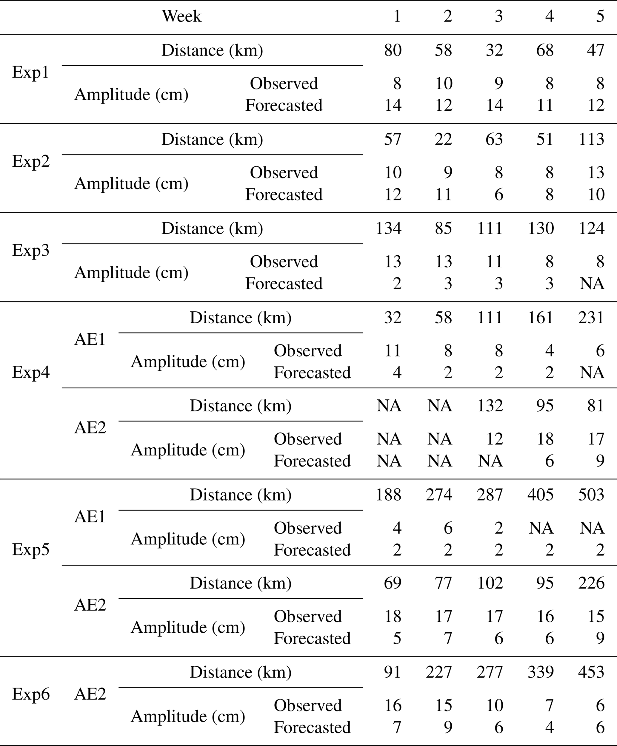
The prediction results of Exp1 are shown in Fig. 8. In Fig. 8a, we can see that the forecast is almost coincident with the satellite observation and the trajectory of drift buoys, indicating that the generated position of AE1 can be well forecasted by the CSCAS. In addition, the initial migration of AE1 can also be forecasted by the CSCAS (see Fig. 8a and f). In order to evaluate the forecasted amplitude of AE1, the amplitude and the distance of eddy centers between the observation and the forecast are also quantified (Table 2, Exp1). From Table 2, Exp1, we can see that the amplitude of forecasting matches well with that of observation, although its amplitude is slightly larger than that of observation. After 4 weeks, the amplitude of the forecast is still close to those of the observation, suggesting that the generation of AE1 can be well predicted by the CSCAS.
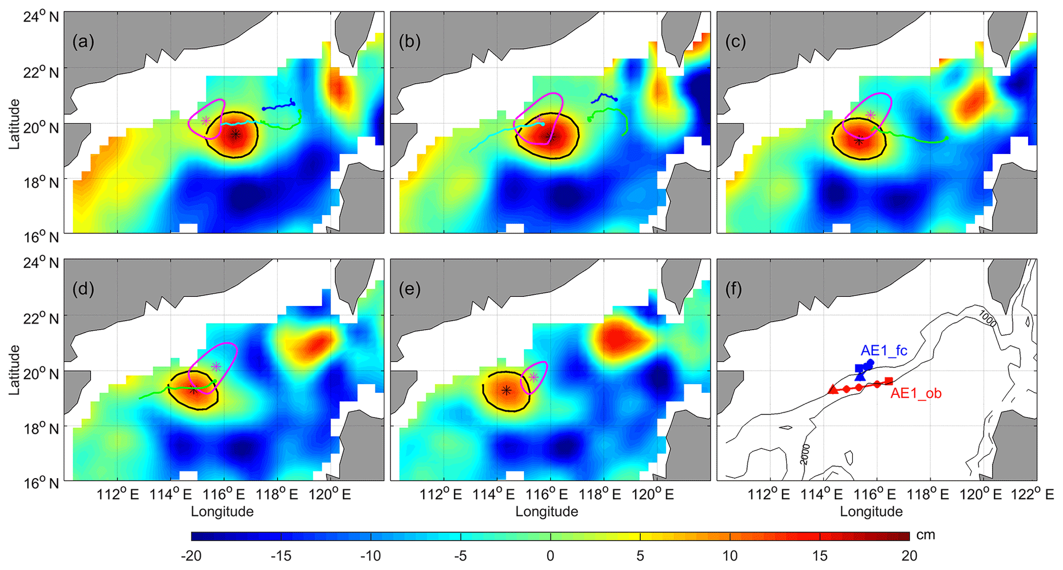
Figure 10Same as Fig. 9, but for Exp3; the experiment period is the 31 December 2003 to the 30 January 2004.
In order to find out whether the development and movement path of AE1 can be predicted after generation, we continue to carry out Exp2. As shown by the observation (Fig. 9), AE1 moves southwestward along the continental shelf with its amplitude decreasing and again increasing after its generation. This observed southwestward movement is also predicted by the CSCAS (see pink closure curve in Fig. 9a–d), although a sudden southwestward movement cannot be well predicted (Fig. 9f). In addition, the first attenuation and then enhancement of AE1 was also predicted by the CSCAS (see Table 2 and Fig. 9b). On the whole, the development and movement path of AE1 can be well predicted by CSCAS for the first 4 weeks after its generation. After that, the errors between observation and prediction increase significantly, and by the fifth week, the distance between the center of the prediction and the observation become larger, more than 100 km (see Fig. 9e).
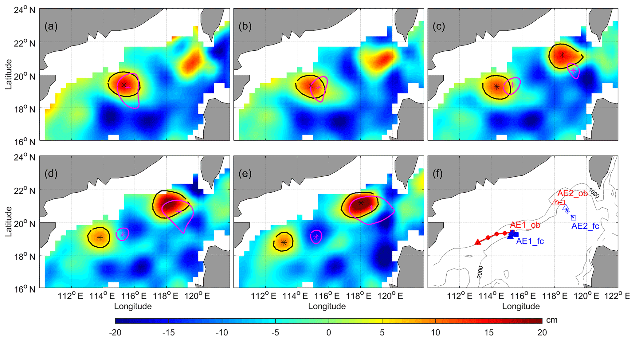
Figure 11Same as Fig. 8, but for Exp4 where the red (blue) dotted line in (f) is the observation (forecast) moving path of AE1 and AE2. The solid (dashed) red lines and solid (hollow) circle are derived from observation SLA for AE1 (AE2); the solid (dashed) blue lines and solid (hollow) circle are derived from forecast SLA during the 21 January to the 20 February 2004.
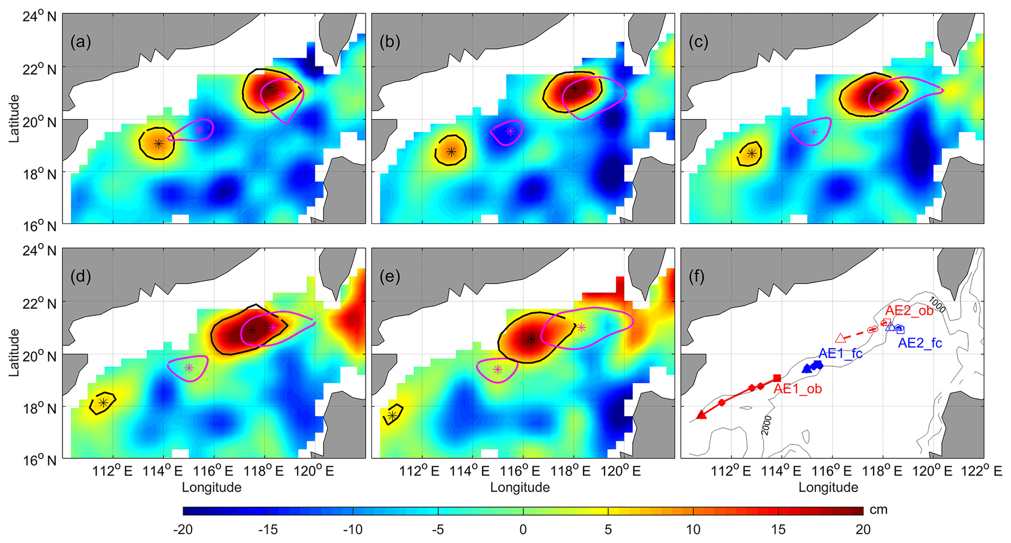
Figure 12Same as Fig. 11, but for Exp5; the experiment period is the 8 February to the 10 March 2004.
For further analysis, we carry out Exp3 to look at whether the continued evolution of AE1 and the generation of AE2 can be predicted. This experiment is carried out based on the initial condition of the assimilation on the 31 December 2003 and the corresponding results are shown in Fig. 10 and Table 2. As shown by the prediction (Fig. 10, Table 2), although with a slightly weak amplitude, the CSCAS can reproduce AE1 after assimilating SLA and SST and predicted its development trend. In addition, the movement path of AE1 cannot be accurately predicted at this period; for instance, the observed AE1 moves directly to the southwest (see solid red line and solid circle in Fig. 10f), but the predicted movement is firstly toward the northeast, then turns to the southwest (see solid blue line and solid circle in Fig. 10f). The generation of AE2 cannot be predicted in Exp3, which may be related to the smaller amplitude (<8 cm) of AE2 during this period.
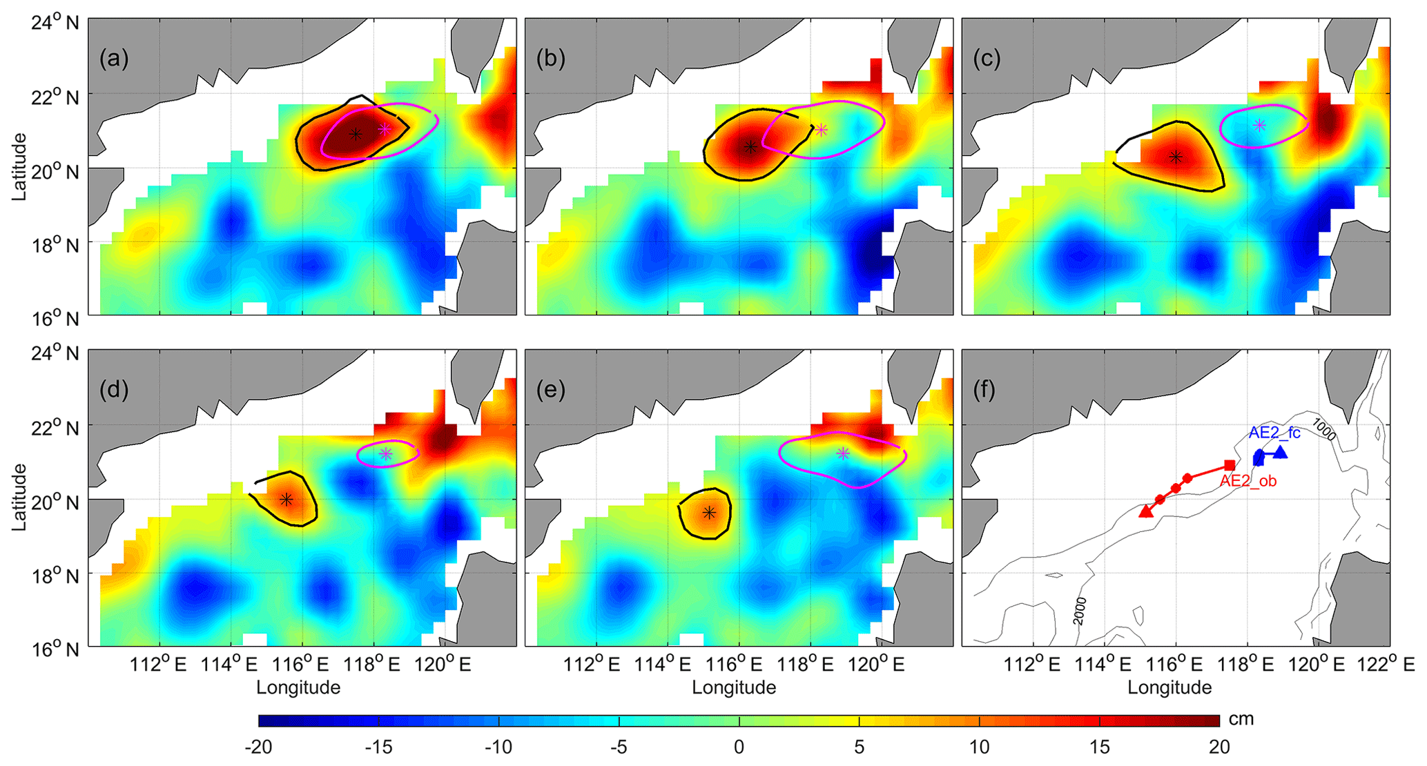
Figure 13Same as Fig. 11, but for Exp6 and AE2; the experiment period is the 29 February to the 30 March 2004.
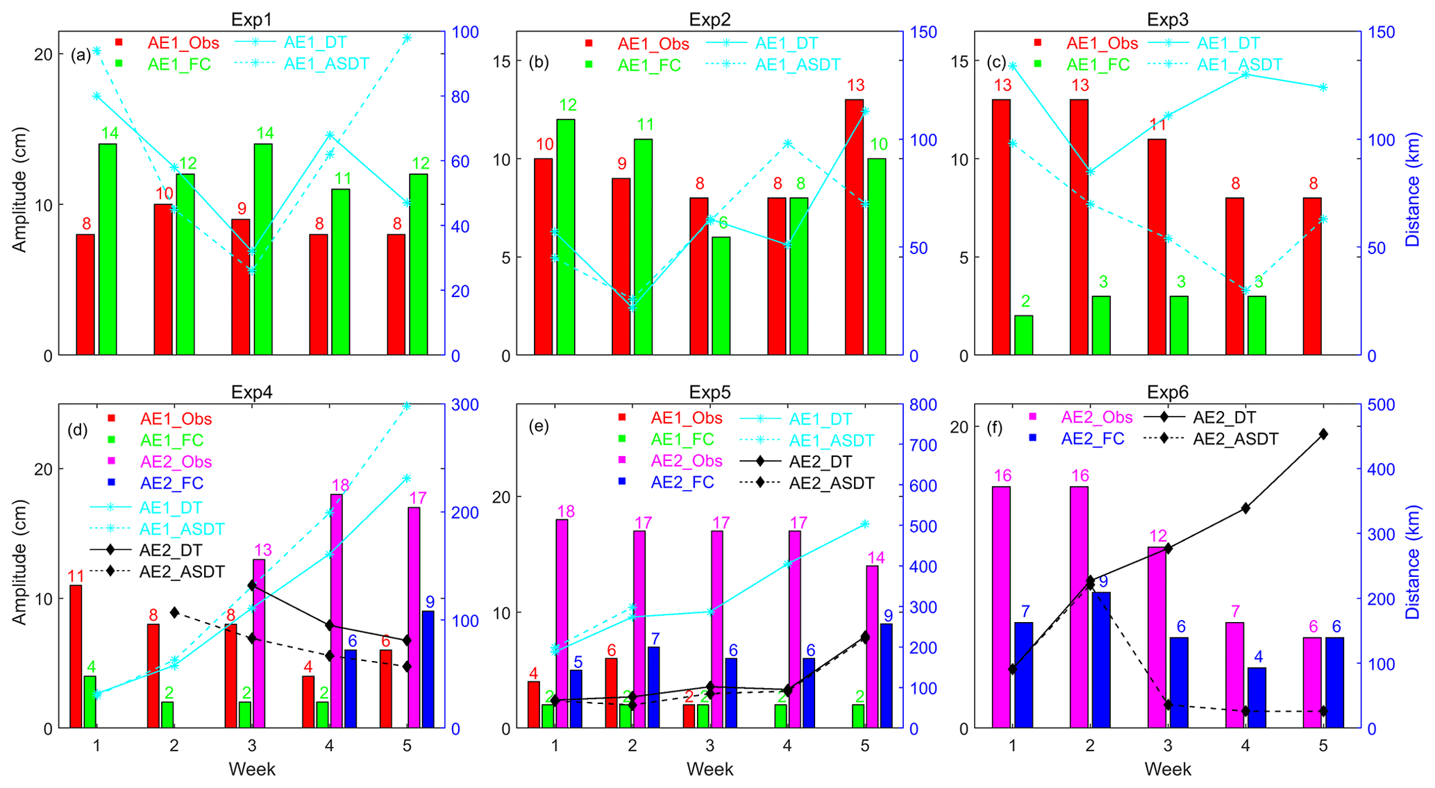
Figure 14The amplitude of AE1 and AE2 derived from observation SLA and the six forecast SLA, and distance of eddy centers between the observation, assimilation, and forecast SLAs, respectively. The red and green histograms indicate the AE1 amplitudes from observation and prediction, respectively. The pink and blue histograms express the AE2 amplitudes from observation and prediction, respectively. The cyan star and solid (dashed) line show the distance of the center between observation and prediction (assimilation) AE1. The black diamond and solid (dashed) line show the distance of the center between observation and prediction (assimilation) AE2.
The purpose of Exp4 is to look at whether the evolution of both AE1 and AE2 can be reasonably predicted. Since this experiment mainly focuses on the evolution of AE1 and AE2, Fig. 11 shows only the evolution of AE2 from the second week after generation, i.e., from the beginning on the 21 January 2004 to the fifth week. As shown in Fig. 11, Table 2, and Fig. 14d, the trends of amplitude variation in both eddies can be well predicted with the decreasing of AE1 and slow increasing of AE2. For AE1, the results of the prediction and observation are very close in the first 2 weeks, with the centers of the two almost coinciding. The central position of the prediction and observation began to deviate after the third week. For AE2, although the amplitude and movement path are not predicted well at its initial stage, the prediction is slowly approaching to the observation during third to fifth week, and distance between the center of the prediction and the observation is reduced from 132 km at the beginning to 81 km at the end (see Fig. 14d, the solid black line).
As mentioned above, the purpose of Exp5 is to investigate whether the decay of AE1 and the continued development of AE2 can be predicted. From Fig. 12, Table 2, and Fig. 14e, we can find that the CSCAS cannot predict the movement path of AE1 well in its decay stage: the distance between the center of the prediction and that of the observation is greater than 188 km, and movement direction of the two is not consistent (see red lines and dots in Fig. 12f). But the evolution and movement direction of AE2 can be well predicted at this stage. The amplitude of observation and prediction of AE2 are getting closer with time (Fig. 14e), although the speed of movement of AE2 given by prediction is slower than that of observation (see dashed blue lines and hollow dots in Fig. 12f).
The aim of Exp6 is to find out if the disappearance of AE1 and AE2 can be both predicted. As described in Fig. 13, the disappearance of AE1 cannot be well predicted owing to the low amplitude (less than 8 cm) of AE1 at this stage. Similarly, the disappearance of AE2 is also less accurately predicted by the CSCAS (Fig. 14f). The observed amplitude of AE2 decays continually at this stage, but the predicted amplitude is almost constant. In addition, there is large deviation of the direction of movement between prediction and observation for AE2 (see the solid red line and dot in Fig. 13f).
In this paper, we carry out a series of assimilation and prediction experiments by the CSCAS to assess the production and predictability of mesoscale eddies in the NSCS, along with observations of satellite observed SST, SLA, and the trajectory data of drift. The comparisons of AE1 and AE2 observations with CSCAS prediction experiments, which assimilate SLA and SST, show that when the amplitudes of mesoscale eddies are higher than 8 cm, the generation, development, decay, and movement of eddies can be well reproduced, but when the amplitude of the mesoscale eddies is lower than 8 cm, the generation and disappearance of mesoscale eddies cannot be well reproduced.
The comparisons of AE1 and AE2 through six prediction experiments with observations also show that the generation, evolution, and movement path of these two eddies with high amplitude (>8 cm or the ANP greater than 2) can be well predicted by the CSCAS, although the generation mechanism of these two eddies is quite different (Wang et al., 2008). However, when the amplitudes of eddies become less than 8 cm, the generation position and the movement path cannot be well predicted by the CSCAS.
Our results suggest that for powerful mesoscale eddies, a good initial condition after assimilating observations can help to improve their reproduction and predictability. As mentioned above, the mesoscale eddies are related to strong nonlinear processes and are not a deterministic response to atmospheric forcing, thus the quality of mesoscale eddies forecast will depend primarily on the quality of the initial conditions. In addition, the ability of the ocean numerical model to faithfully represent the ocean physics and dynamics is also crucial. Although data assimilation, which combines observations with the numerical model, can provide good initial conditions, it cannot make up for limitations of numerical model algorithms and in their resolution. Hence for high-resolution operational oceanography, numerical models need to be improved using more accurate numerical algorithms and resolution especially in the weakly stratified regions or on the continental shelf.
Furthermore, so far most of the information about the ocean variability is obtained remotely from satellites (SSH and SST), information about the subsurface variability is very rare. Although a substantial source of subsurface data is provided by the vertical profiles (i.e., expendable bathythermographs, conductivity temperature depth, and Argo floats), the datasets are still not sufficient to determine the state of the ocean. In addition, in order to accurately assimilate the SSH anomalies from satellite altimeter data into the numerical model, it is necessary to know the oceanic mean SSH over the time period of the altimeter observations (Xu et al., 2011; Rio et al., 2014). This is also a big challenge because the earth's geoid is not presented with sufficient spatial resolution when assimilating SSH in an eddy-resolving model. With the advent of the SWOT (Surface Water and Ocean Topography) satellite mission in 2020, it should be possible to better resolve and forecast the mesoscale features in eddy-resolving ocean-forecasting systems.
The data that support the findings of this study are available from the corresponding author upon reasonable request.
All authors contributed equally to this work. DX wrote the main paper, run the numerical model and processed the model output. WZ focused on the processing of observed data. YY provided the idea of this work and revised the manuscript. All authors discussed the results and implications and commented on the manuscript at all stages.
The authors declare that they have no conflict of interest.
This study is supported by the Marine Science and Technology Foundation of
the South China Sea branch, State Oceanic Administration (grant 1447), the
National Key Research and Development Program of China (2016YFC1401407), the
project of Global Change and Air-Sea interaction under contract no.
GASI-03-IPOVAI-04, the National Natural Science Foundation of China (grant
nos. 41731173, 41776037 and 41276027), and the China Scholarship Council
(award to Xu Dazhi for 1 year study abroad at Nansen Environmental and Remote
Sensing Center).
Edited by: John M.
Huthnance
Reviewed by: two anonymous referees
Bleck, R.: An oceanic general circulation model framed in hybrid isopycnic cartesian coordinates, Ocean Model., 4, 55–88, 2002.
Boyer, T. P., Levitus, S., Antonov, J. I., Locarnini, R. A., and Garcia, H. E.: Linear trends in salinity for the World Ocean, 1955–1998, Geophys. Res. Lett., 32, 67–106, 2005.
Chassignet, E. P., Hurlburt, H. E., Smedstad, O. M., Halliwell, G. R., Hogan, P. J., Wallcraft, A. J., Baraille, R., and Bleck, R.: The HYCOM (Hybrid Coordinate Ocean Model) data assimilative system, J. Marine Syst., 65, 60–83, 2007.
Chelton, D. B., Schlax, M. G., and Samelson, R. M.: Global observations of nonlinear mesoscale eddies, Prog. Oceanogr., 91, 167–216, 2011.
Cheng, X. H., Qi, Y. Q., and Wang, W. Q.: Seasonal and Interannual Variabilities of Mesoscale Eddies in South China Sea, J. Trop. Oceanogr., 24, 51–59, 2005.
Counillon, F. and Bertino, L.: Ensemble Optimal Interpolation: multivariate properties in the Gulf of Mexico, Tellus, 61A, 296–308, 2009.
Dai, A. and Trenberth, K. E.: Estimates of freshwater discharge from continents: latitudinal and seasonal variations, J. Hydrometeorol., 3, 660–685, 2002.
Ducet, N., LeTraon, P. Y., and Reverdin, G.: Global high-resolution mapping of ocean circulation from TOPEX/Poseidon and ERS-1 and-2, J. Geophys. Res., 105, 19477–19498, 2000.
Frenger, I., Gruber, N., Knutti, R., and Münnich, M.: Imprint of Southern Ocean eddies on winds, clouds and rainfall, Nat. Geosci., 6, 608–612, 2013.
Fu, L.-L., Chelton, D. B., Traon, P.-Y. L., and Rosemary, M.: Eddy dynamics from satellite altimetry, Oceanography, 23, 14–25, 2010.
Halliwell, J. G. R.: Evaluation of vertical coordinate and vertical mixing algorithms in the HYbrid-Coordinate Ocean Model (HYCOM), Ocean Model., 7, 285–322, 2004.
Halliwell, J. G. R., Bleck, R., and Chassignet, E. P.: Atlantic Ocean simulations performed using a new Hybrid Coordinate Ocean Model (HYCOM), EOS, Fall AGU Meeting, Trans. AGU, 1998.
Halliwell, J. G. R., Bleck, R., Chassignet, E. P., and Smith, L. T.: Mixed layer model validation in Atlantic Ocean simulations using the Hybrid Coordinate Ocean Model (HYCOM), EOS, 80, OS304, 2000.
Hamilton, P., Fargion, G. S., and Biggs, D. C.: Loop Current eddy paths in the western Gulf of Mexico, J. Phys. Oceanogr., 29, 1180–1207, 1999.
Han, Y.–J.: A numerical world ocean general circulation model: Part II. A baroclinic experiment, Dynam. Atmos. Oceans, 8,141–172, 1984.
Huang, B. Q., Hua, J., Xu, H. Z., and Wang, D.: Phytoplankton community at warm eddies in the northern South China Sea in winter 2003/2004, Deep-Sea Res. Pt. II, 57, 1792–1798, 2010.
Jia, Y., Liu, Q., and Liu, W.: Primary studies of the mechanism of eddy shedding from the Kuroshio bend in Luzon Strait, J. Oceanogr., 61, 1017–1027, 2005.
Kara, A. B., Rochford, P. A., and Hurlburt, H. E.: Air-sea flux estimates and the 1997–1998 ENSO event, Bound.-Lay. Meteorol., 103, 439–458, 2002.
Large, W. G., McWilliams, J. C., and Doney, S. C.: Oceanic vertical mixing: a review and a model with a nonlocal boundary layer parameterization, Rev. Geophys., 32, 363–403, 1994.
Legates, D. R. and Willmott, C. J.: Mean seasonal and spatial variability in gauge-corrected, global precipitation, Int. J. Climatol., 10, 111–127, 1990.
Li, L., Nowlin, W. D., and Su, J, L.: Anticyclonic rings from the Kuroshio in the South China Sea, Deep-Sea Res. Pt. I, 45, 1469–1482, 1998.
Li, Q. Y. and Sun, L.: Technical Note: Watershed strategy for oceanic mesoscale eddy splitting, Ocean Sci., 11, 269–273, https://doi.org/10.5194/os-11-269-2015, 2015.
Li, Q. Y., Sun, L., Liu, S.-S., Xian, T., and Yan, Y. F.: A new mononuclear eddy identification method with simple splitting strategies, Remote Sens. Lett., 5, 65–72, https://doi.org/10.1080/2150704X.2013.872814, 2014.
Li, Q.-Y., Sun, L., and Lin, S.-F.: GEM: a dynamic tracking model for mesoscale eddies in the ocean, Ocean Sci., 12, 1249–1267, https://doi.org/10.5194/os-12-1249-2016, 2016.
Li, X. C.: Applying a new localization optimal interpolation assimilation module to assimilate sea surface temperature and sea level anomaly into the Chinese Shelf/Coastal Seas model and carry out hindcasted experiment, Graduate University of the Chinese Academy of Sciences, Beijing, China, 92 pp., 2009.
Li, X. C., Zhu, J., Xiao, Y. G., and Wang, R.: A Model-Based Observation Thinning Scheme for the Assimilation of High-Resolution SST in the Shelf and Coastal Seas around China, J. Atmos. Ocean. Tech., 27, 1044–1058, 2010.
Liu, Z., Yang, H. J., and Liu, Q.: Regional dynamics of seasonal variability of sea surface height in the South China Sea, J. Phys. Oceanogr., 31, 272–284, 2001.
Morrow, R. and Traon, P.-Y. L.: Recent advances in observing mesoscale ocean dynamics with satellite altimetry, Adv. Space Res., 50, 1062–1076, 2012.
Oey, L. T., Ezer, T., and Lee, H. C.: Loop Current, rings and related circulation in the Gulf of Mexico: a review of numerical models, in: Circulation in the Gulf of Mexico: Observations and Models, Volume 161, American Geophysical Union, 31–56, 2005.
Oke, P. R., Allen, J. S., Miller, R. N., Egbert, G. D., and Kosro, P. M.: Assimilation of surface velocity data into a primitive equation coastal ocean model, J. Geophys. Res.-Oceans, 107, 5-1–5-25, 2002.
Oke, P. R., Brassington, G. B., Griffin, D. A., and Schiller, A.: Ocean data assimilation: a case for ensemble optimal interpolation, Aust. Meteorol. Ocean., 59, 67–76, 2010.
Reynolds, R. W., Smith, T. M., Liu, C., Chelton, D. B., Casey, K. S., and Schlax, M. G.: Daily High-Resolution Blended Analyses for Sea Surface Temperature, J. Climate, 20, 5473–5496, 2007.
Rio, M. H., Mulet, S., and Picot, N.: Beyond GOCE for the ocean circulation estimate: Synergetic use of altimetry, gravimetry, and in situ data provides new insight into geostrophic and Ekman currents, Geophys. Res. Lett., 41, 8918–8925, 2014.
Treguier, A. M., Chassignet, E. P., Boyer, A. L., and Pinardi, N.: Modeling and forecasting the “weather of the ocean” at the mesoscale, J. Mar. Res., 75, 301–329, 2017.
Uppala, S., Kallberg, P., Simmons, A. J., Andrae, U., Da Costa Bechtold, V., Fiorino, M., Gibson, J. K., Haseler, J., Hernandez, A., Kelly, G. A., Li, X., Onogi, K., Saarinen, S., Sokka, N., Allan, R. P., Andersson, E., Arpe, K., Balmaseda, M. A., Beljaars, A. C. M., Van De Berg, L., Bidlot, J., Bormann, N., Caires, S., Chevallier, F., Dethof, A., Dragosavac, M., Fisher, M., Fuentes, M., Hagemann, S., Hólm, E., Hoskins, B. J., Isaksen, L., Janssen, P. A. E. M., Jenne, R., Mcnally, A. P., Mahfouf, J.-F., Morcrette, J.-J., Rayner, N. A., Saunders, R. W., Simon, P., Sterl, A., Trenberth, K. E., Untch, A., Vasiljevic, D., Viterbo, P., and Woollen, J.: The EAR-40 re-analysis, Q. J. Roy. Meteor. Soc., 131, 2961–3012, 2005.
Vos, M. D., Backeberg, B., and Counillon, F.: Using an eddy-tracking algorithm to understand the impact of assimilating altimetry data on the eddy characteristics of the Agulhas system, Ocean Dynam., 68, 1071-1091, 2018.
Wang, D. X., Zhou, F. Z., and Qin Z. H.: Numerical simulation of the upper ocean circulation with two-layer model, Acta Oceanol. Sin., 18, 30–40, 1996.
Wang, D., Xu, H., Lin, J., and Hu, J.: Anticyclonic eddies in the northeastern South China Sea during winter 2003/2004, J. Oceanogr., 64, 925–935, https://doi.org/10.1007/s10872-008-0076-3, 2008.
Wang, G., Su, J., and Chu, P. C.: Mesoscale eddies in the South China Sea observed with altimeter data, Geophys. Res. Lett., 30, 2121, https://doi.org/10.1029/2003GL018532, 2003.
Wang, Z., Li, Q., Sun, L., Li, S., Yang, Y., and Liu, S.: The most typical shape of oceanic mesoscale eddies from global satellite sea level observations, Front. Earth Sci., 9, 202–208, https://doi.org/10.1007/s11707-014-0478-z, 2015.
Woodham, R. H., Alves, O., Brassington, G. B., Robertson, R., and Kiss, A.: Evaluation of ocean forecast performance for Royal Australian Navy exercise areas in the Tasman Sea, J. Oper. Oceanogr., 8, 147–161, 2015.
Woodruff, S. D., Slutz, R. J., Jenne, R. L., and Steurer, P. M.: A comprehensive ocean-atmosphere data set, B. Am. Meteorol. Soc., 68, 1239–1250, 1987.
Wu, C. R. and Chiang, T. L.: Mesoscale eddies in the northern South China Sea, Deep-Sea Res. Pt. II, 54, 1575–1588, 2007.
Xiao, X. J., Wang, D. X., and Xu, J.-J.: The assimilation experiment in the southwestern South China Sea in summer 2000, Chinese Sci. Bull., 51, 31–37, 2006.
Xie, J., Counillon, F., Zhu, J., and Bertino, L.: An eddy resolving tidal-driven model of the South China Sea assimilating along-track SLA data using the EnOI, Ocean Sci., 7, 609–627, https://doi.org/10.5194/os-7-609-2011, 2011.
Xie, J. P., Bertino, L., Cardellach, E., Semmling, M., and Wickert, J.: An OSSE evaluation of the GNSS-R altimetery data for the GEROS-ISS mission as a complement to the existing observational networks, Remote Sens. Environ., 209, 152–165, 2018.
Xu, D. Z., Li, X. C., Zhu, J., and QI, Y. Q.: Evaluation of an ocean data assimilation system in the marginal seas around China, with a focus on the South China Sea, Chin. J. Oceanol. Limn., 29, 414–426, 2011.
Xu, D. Z., Zhu, J., Qi, Y. Q., LI, X. C., and Yan, Y. F.: Impact of mean dynamic topography on SLA assimilation in an eddy-resolving model, Acta Oceanol. Sin., 31, 11–25, 2012.
Yan, C. X., Zhu, J., and Zhou, G. Q.: Impacts of XBT, TAO, altimetry and ARGO observations on the tropic Pacific Ocean data assimilation, Adv. Atmos. Sci., 24, 383–398, 2007.
Yang, K., Shi, P., Wang, D. X., You, X. B., and Li, R. F.: Numerical study about the mesoscale multi-eddy system in the northern South China Sea in winter, Acta Oceanol. Sin., 22, 27–34, 2000.
Yang, S., Xing, J., Chen, D., and Chen, S.: A modelling study of eddy-splitting by an island/seamount, Ocean Sci., 13, 837–849, https://doi.org/10.5194/os-13-837-2017, 2017.
Yuan, S. Y. and Wang, Z. Z.: Topography forced Rossby waves in the section from Xisha to Dongsha Islands, Tropic Oceano., 5, 1–6, 1986.
Zhai, X., Johnson, H. L., and Marshall, D. P.: Significant sink of ocean-eddy energy near western boundaries, Nat. Geosci., 3, 608–612, 2010.
Zhu, J.: Overview of Regional and Coastal Systems, Chapter 17 in Operational Oceanography in the 21st Century, edited by: Schiller, A. and Brassington, G. B., 727 pp., Springer Science, Business Media B.V, Dordrecht, 2011.
Zhuang, W., Du, Y., Wang, D. X., Xie, Q., and Xie, S.: Pathways of mesoscale variability in the South China Sea, Chin. J. Oceanol. Limn., 28, 1055–1067, 2010.