Some aspects of the deep abyssal overflow between the middle and southern basins of the Caspian Sea

The present study investigates the deep gravity current between the middle and southern Caspian Sea basins caused by the density difference of deep waters. Oceanographic data, a numerical model and a dynamic model are used to consider the structure of this Caspian Sea abyssal overflow. The CTD data are obtained from UNESCO, and the three-dimensional COHERENS ocean model results are used to study the abyssal currents in the southern basin of the Caspian Sea.

The deep overflow is driven by the density difference, which is mainly owing to the temperature difference, between the middle and southern basins, especially in winter. Due to cold weather in the northern basin, water sinks at high latitudes and after filling the middle basin it overflows into the southern basin. As the current passes through the Absheron Strait (or sill), we use the analytic model of Falcini and Salusti (2015) for the overflow gravity current to estimate the changes in the vorticity and potential vorticity of the flow over the Absheron sill; the effects of entrainment and friction are also considered. Due to the importance of the overflow with respect to deep water ventilation, a simple dynamical model of the boundary currents based on the shape of the Absheron Strait is used to estimate typical mass transport and flushing time; the flushing time is found to be about 15 to 20 years for the southern basin of the Caspian Sea. This timescale is important for the region's ecosystem and with respect to the impacts of pollution due to oil exploration. In addition, by reviewing the drilled oil and gas wells in the Caspian Sea, the results show that the deep overflow moves over some of these wells. Thus, the deep flow could be an important factor influencing oil pollution in the deeper region of the southern Caspian Sea.

1 Introduction

Baroclinic currents play an important role in the ocean and sea circulations, especially in the deep waters of the ocean. Because these currents are important with respect to deep water ventilation in the oceans, they have an integral role in thermohaline circulation. A driving mechanism for the circulation is the cooling of surface waters at high latitudes and the consequent formation of deep waters due to the sinking of cooled salty water masses (Fogelqvist et al., 2003).

Cooling in polar seas (Dickson et al., 1990) and evaporation in marginal seas (Baringer and Price, 1997) form dense waters that sink to form deep water masses. For example, dense water from the deep convective regions of the North Atlantic produces a thermohaline overturning circulation signature that can be seen as far away as the Pacific and Indian oceans (Girton et al., 2003). In the global sense, bottom-trapped currents play an integral role in thermohaline circulation and are a vehicle for the transport of heat, salt, oxygen and nutrients over great distances and depths. Mixing and exchange processes between along-slope currents at the continental shelves and deep ocean water can also affect the thermohaline circulations. Huthnance (1995) reviewed the processes involved in such near-shelf circulations and pointed out such flows around the world that may lead to the formation of mesoscale eddies as they become unstable while moving along the sloped boundary. The ability of abyssal flows to transport and deposit sediments is also of geological interest (Smith, 1975).

As thermohaline circulation causes the ventilation of deep ocean water, it is important not only in open seas and ocean but also with respect to semi-closed and closed basins ventilation, e.g., the Caspian Sea. The study of thermohaline dynamics and circulation has also been of interest to other scientists such as climate researchers. The dynamics of such dense currents on slopes have been modeled in the past both theoretically and experimentally starting with Ellison and Turner (1959), Britter and Linden (1980), and a review on gravity currents that can be found in Griffiths (1986).

The Caspian Sea, the world's largest inland enclosed water body, consists of three basins – namely the northern basin (shallow, with a mean depth of about 10 m and covering 80 000 km²), the middle basin (rather deep, with a mean depth of about 200 m, maximum depth 788 m and covering 138 000 km²) and the southern basin (deep, with a mean depth of 350 m, a maximum depth of 1025 m and covering 164 840 km²) – and is located between 36.5 and 47.2^∘ N and 46.5 and 54.1^∘ E (Aubrey et al., 1994; Aubrey, 1994). The depth varies greatly over this sea (Ismailova, 2004; Fig. 1). The northern basin, after a sudden depth transition at the shelf edge, reaches the middle basin. The middle and southern basins are divided by the Absheron Strait, or Absheron sill, which has a maximum depth of 180 m. The western slopes of the two deeper basins are fairly steep compared with the eastern slope (Gunduz and Özsoy, 2014). Peeters et al. (2000) estimated the ages of waters of the Caspian Sea basins while considering the exchange between the middle and southern basins, based on chemical tracers, and found typical ages of about 20 to 25 years depending on the exchange rates. The exchange rate between the middle and southern basins seems to vary year by year and is dominated by atmospheric forcing (and sea level change).

The Caspian Sea is enclosed with weak tides and its circulation is mainly due to wind and buoyancy, although some wave-driven flows also occur in coastal regions (Bondarenko, 1993; Ghaffari and Chegini, 2010; Ghaffari et al., 2013; Ibrayev et al., 2010; Terziev et al., 1992). The seasonal circulation based on a coupled sea hydrodynamics, air–sea interaction and sea-ice thermodynamics model of the Caspian Sea was investigated by Ibrayev et al. (2010) and Gunduz and Özsoy (2014). The effect of freshwater inflow to the Caspian Sea on the seasonal variations of salinity and the surface circulation (or flow) pattern of the Caspian Sea has also been studied using HYCOM model (e.g., Kara et al., 2010). These studies have indicated that there are signs of sinking water in cold season in the northeastern parts of the middle basin of this sea . Such deep convection could be a part of the thermocline circulations, affected by the topography of the side walls of the middle and southern basins; these deep topographically influenced rotating flows could constitute parts of the abyssal circulation of the Caspian Sea.

The main aim of the present work was to study the deep abyssal overflow in the Caspian Sea, which has only been touched on in previous studies. To achieve this, we used observational data and numerical simulations to show that the overflow could exist over the Absheron sill. Firstly, we used observational data to understand the feasibility of the deep flow in this basin; however, the resolution of the observational data was very low in order to cover all of the intended applications discussed in the paper. Hence, the use of a numerical model helped us better understand the Absheron sill deep overflow. This paper is divided into three main parts based on the goals of the paper. Section 2 focuses on the existence of the deep overflow in the Caspian Sea using some observations and numerical simulations, as there has been little research on deep flow in this region (Peeters et al., 2000). In the course of this section, the accuracy of the model simulations is considered by comparing the model results with observational data. Section 3 concentrates on the dynamics of the outflow when moving through the Absheron Strait into the southern basin. Although there are many aspects of the dynamics of the flow, the vorticity and potential vorticity will be specifically considered in this section. In Sect. 4, the importance of the abyssal overflow will be indicated and the volume of this flow and the associated flushing time of the southern Caspian Sea basin will be calculated using a simple model for the overflow over the Absheron sill.

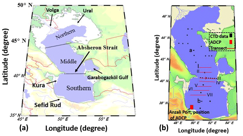
Figure 1 (a) Schematic diagram of the Caspian Sea showing the locations of the most important rivers namely the Volga, Ural, Kura and Sefid Rud; the Garabogazköl Gulf and the Absheron Strait are also shown on the map. (b) The locations of the CTD and ADCP measurements and the geographic position of the transects are shown. The CTD casts are for 42 stations for the month of September in both 1995 and 1996. The CTD stations (labeled a and b) are emphasized because the physical properties of the waters for these stations are presented in Fig. 2a and b. ADCP data are recorded from November 2004 to the end of January 2005 to validate the numerical simulations.

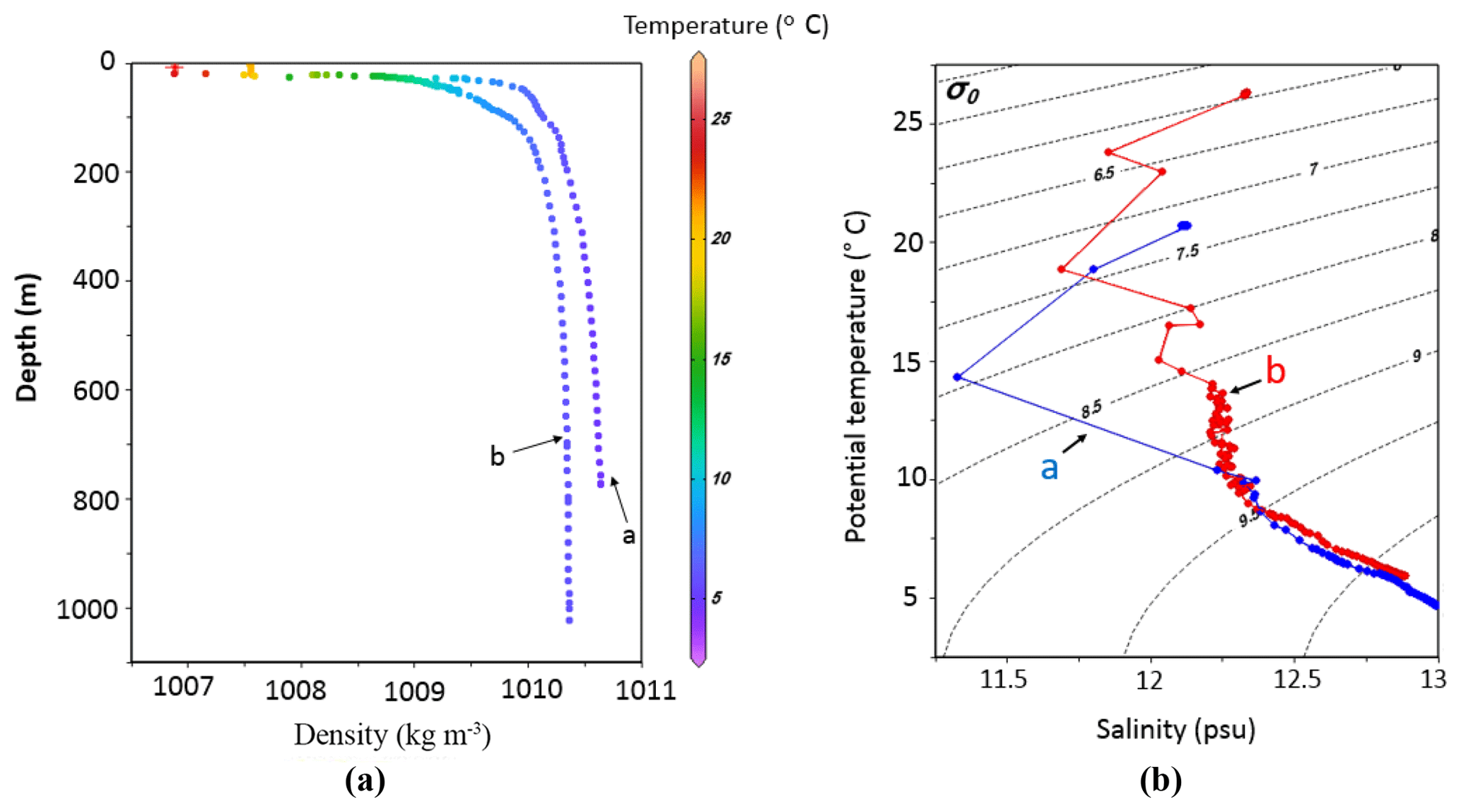
Figure 2 (a) Comparison of density between stations a and b (middle and southern basins, see Fig. 1b) indicating the difference in density (∼0.5 kg m⁻³) between the two basins. (b) A T–S diagram for stations a and b to show differences in temperature and salinity, particularly in deep water. To plot this diagram, the potential temperature and potential density anomaly (σ₀) are calculated from the CTD data. The T–S diagram confirms the differences in density in deep water for σ₀>10 kg m⁻³.

2 Data used and an outline of the research method

2.1 Observational data

The data used in this study were mainly collected by the International Atomic Energy Agency (IAEA), in September of 1995 and 1996 (Peeters et al., 2000). The data were collected at 42 stations using an exploration ship, namely the Hajef. The 1995 data were from 13 stations, whereas the 1996 data were from 29 stations (Fig. 1). In this work, temperature, salinity and density diagrams are first plotted for all stations. Both data sets indicate the differences between the densities of deep waters of the middle and southern basins. For example, Fig. 2a shows the density differences between stations a and b (Fig. 1b) to be about 0.5 kg m⁻³. To facilitate a better understanding, a T–S (temperature–salinity) diagram is plotted to investigate the contribution of temperature and salinity to this density difference. Based on the T–S diagram, the water in the middle basin is both cooler and saltier than that of the southern basin, particularly in the deeper regions. Hence, the denser deeper water of the middle basin with respect of that of southern basin could lead to deep abyssal overflow between the two basins over the sill of the Absheron Strait, which separates the middle and southern basins. The temperature, salinity and density transect across the Absheron Strait, as shown in Fig. 3a and  b, also shows evidence of the deep abyssal overflow moving from the middle to the southern basin. As the sloped isopycnals are similar to those of isotherms, it seems that the buoyancy that drives the flow is mainly due to the temperature difference. However, unfortunately, the horizontal resolution of the data used is not good enough to show detailed patterns of temperature, salinity and density of the overflow (see below).

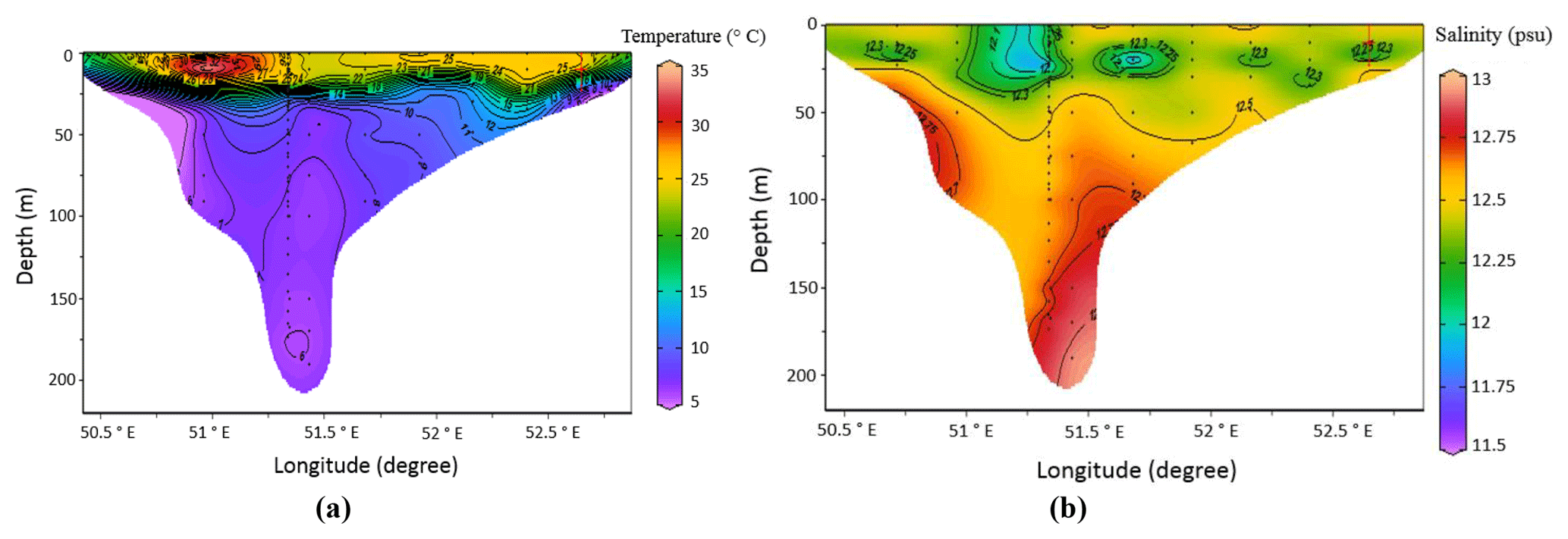
Figure 3 Cross sections of temperature and salinity across the strait at transect I (across the Absheron Strait over the sill) in September from observational data; dots show the locations of measurements.

Figure 4 Comparison between density fields across the strait in transect I, in September from observational data (a) and from the numerical model (b). For observational data, dots show the locations of measurements. For a better understanding of the spacing of the CTD stations, the distance is plotted in kilometers on the top of Fig. 4a. The cross sections are about the same, but the differences between the two transects near the bottom, particularly in the west of the strait, are mainly due to the low resolution of observational data (a). The numerical transect clearly shows the boundary trapped overflow for which two isopycnals near the bottom are highlighted (b).

The horizontal resolution of the observational data is very coarse for showing the overflow. For example, Fig. 4a indicates that the width of the strait is about 200 km, and we have just nine CTD stations. This means that the average distance between two stations is 23 km; however, unfortunately, in the most important area of the strait (the western region) the distance between two stations is 30–35 km. As a result, we have problems showing the structure of the flow. More fine-resolution data and data for different months are required to compare the cross sections of the flow for different months. Hence, due to the lack of good measurements around the strait between the two main basins of the Caspian Sea, we are compelled to use numerical simulations for the study of deep overflow at the Absheron sill, including its seasonal variability. This also includes some general aspects of the circulations in the Caspian Sea.

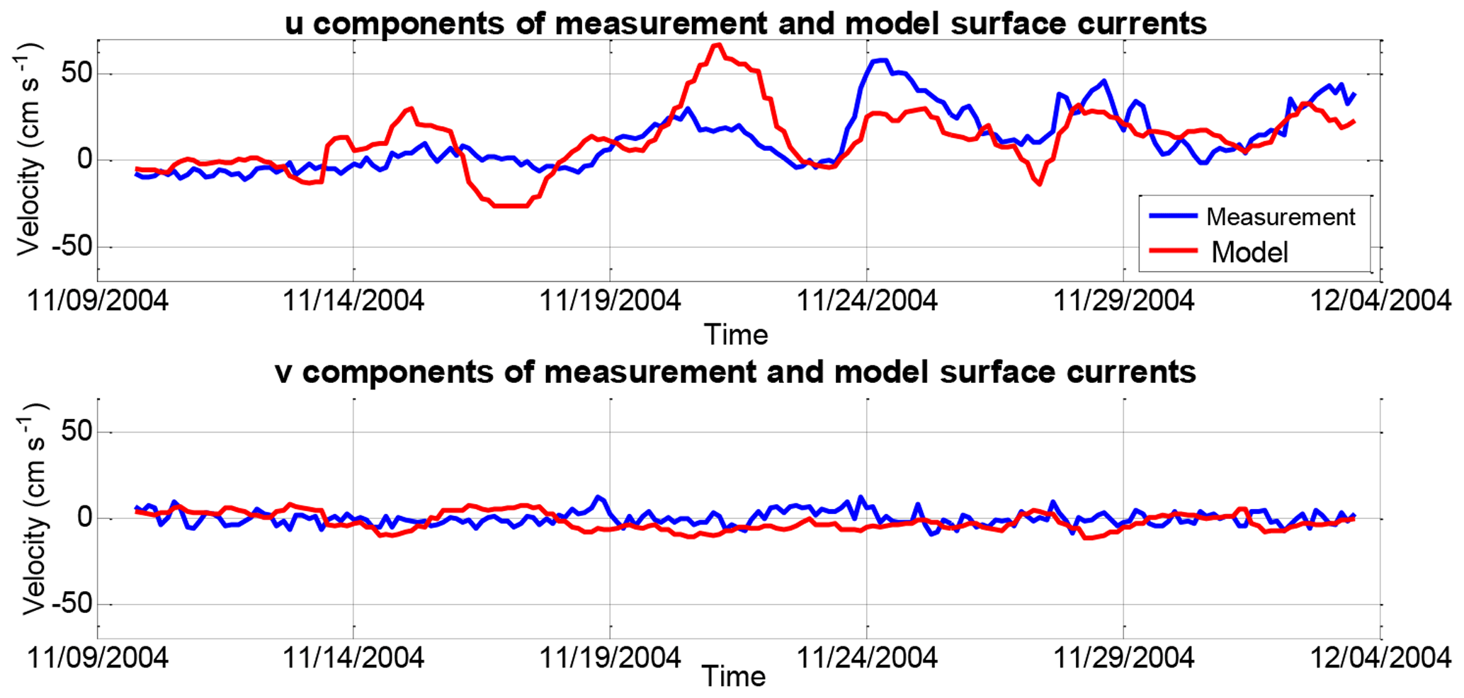
Figure 5 Comparison of numerical model results of surface current components and observations near the Sefid Rud River and the Anzali Port (Shiea et al., 2016).

Figure 6 Cross section of the mean velocity (m s⁻¹) in transect I, obtained from model simulations, (a) for January and (b) May. This deep flow is moving southwards.

2.2 Some general features of the COHERENS numerical model, and its boundary and initial conditions

The COHERENS (Coupled Hydrodynamical Ecological model for Regional Shelf seas; Luyten et al., 1999) numerical model was used for the simulations in this study. COHERENS uses a vertical sigma coordinate and the hydrostatic incompressible version of the Navier–Stokes equations with the Boussinesq approximation and equations of temperature and salinity. The model uses an Arakawa C-grid (Arakawa and Suarez, 1983), and equations are solved numerically using the mode-splitting technique. The grid size is $\mathrm{0.046}{}^{\circ }\times \mathrm{0.046}$^∘ in the horizontal, typically 5 km, and 30σ layers, labeled k (the bottom layer is 1 and the surface layer is 30). The coastlines and bathymetry data with ${\mathrm{0.5}}^{\prime }\times {\mathrm{0.5}}^{\prime }$ (30 s) resolution were acquired from GEBCO, although they were interpolated and smoothed slightly.

The model was initialized for winter (January) using monthly mean temperature and salinity climatology, obtained from Kara et al. (2010); it was forced by 6-hourly wind data, acquired from the European Centre for Medium-Range Weather Forecasts (ECMWF) (Mazaheri et al., 2013) and air pressure and temperature with a ${\mathrm{0.5}}^{\circ }\times {\mathrm{0.5}}^{\circ }$ resolution acquired from ECMWF (ERA-Interim) reanalysis. The precipitation rate, cloud cover and relative humidity (${\mathrm{2.5}}^{\circ }\times {\mathrm{2.5}}^{\circ }$) were derived from NCEP/NCAR reanalysis data. The river inflows (from the Global Runoff Data Centre) were also included. The time steps of the barotropic and baroclinic modes were 15 and 150 s, respectively. The total simulation time was 5 years (from 2000 to 2004 inclusive) with 6 h varying meteorological forcing; the results of the last year are shown. The results of the numerical model are validated by ADCP data of the estuary between the Sefid Rud River and Anzali Port (Figs. 1, 5). These data are collected by the National Institute of Oceanography and Atmospheric Sciences, from November 2004 to the end of January 2005 (Shiea et al., 2016). The data were recorded by a RCM9 current meter (at the ADCP station) at three depths on a mooring: near the surface, at 50 m and at 200 m (Ghaffari and Chegini, 2010). The lack of observational data is the main obstacle with respect to checking the accuracy of the model results thoroughly. It would be more useful to have data from the Absheron sill for the model validation. However, ADCP data from near the Iranian coast was the only available option for model validation. For this reason, the model simulations are for 5 years, and the results of the last year of simulations are validated using ADCP data for some months.

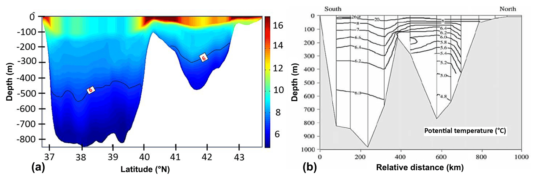
Figure 7 Comparison of the north–south cross sections of mean temperature obtained from model simulation (a) and Peeters et al. (2000) measurements (b) during September. The 6 ^∘C isotherm is marked for easier comparison.

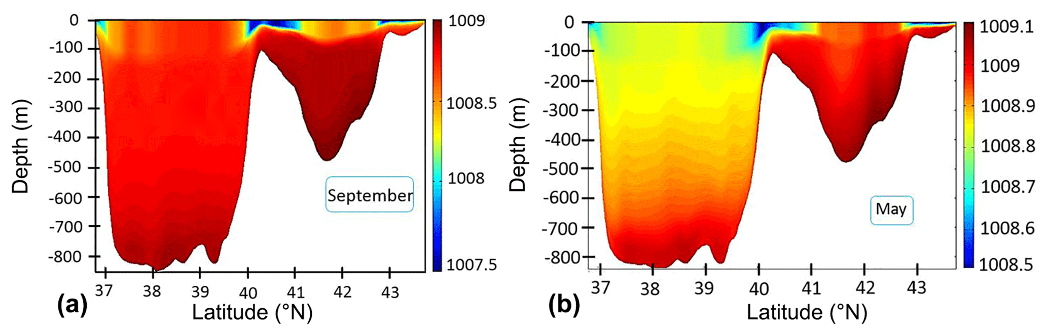
Figure 8 Cross sections (north–south) of the mean density obtained from model simulation during September (a) and May (b).

The simulation results of mean and long-term variations of surface velocity components are quite consistent with observations. This similarity is related to the timing of flow variations rather than the velocity magnitudes. The difference in velocity between observations and model simulations stems from some of the assumptions made and the resolution used in the model, as can be expected. The distance between two adjacent grid points in the model is about 5 km, and the ADCP data are for a point in between the two adjacent grid points; therefore, interpolation is used to compare the model results with data at the location of observations.

The observational data are indicative of the existence of a deep overflow over the Absheron sill (Fig. 4a). The numerical simulations also show that a deep overflow clearly exists over the sill (Figs. 4b, 6, 14), which we examine here in more detail. Typical numerical results of the deep overflow between the middle and southern basins of the Caspian Sea (the flow in the northern basin is not shown as it is too shallow) for May and December of 2004, after 4 years of model warm-up, are shown in Figs. 6–8 and 14. The deep narrow flow in the middle basin in addition to the overflow over the Absheron sill and in the northwestern boundary of the southern basin are clearly observed.

2.3 Comparison of numerical simulations with observations

The main reason for the existence of deep flow in the Caspian Sea seems to be the temperature differences between the northern and southern basins. The sea surface temperature (SST) in the northern basin ranges from below 0 ^∘C under frozen ice in winter to 25–26 ^∘C in summer, while more moderate variability occurs in the southern basin with the sea surface temperature ranging from 7–10 ^∘C in winter to 25–29 ^∘C in summer (Ibrayev et al., 2010). This shows that the water in the northern basin cools in the cold seasons so that it freezes. Conversely, the Caspian Sea has low salinity water, and in deeper regions salinity varies little with depth (12.80–13.08 PSU), meaning that the density stratification largely depends on temperature variation (Terziev et al., 1992). As the northern shallow waters of the Caspian Sea are subjected to high evaporation in summer, in the following cold seasons these waters become dense and start to sink, mainly on the northeastern side of this sea (Gunduz and Özsoy, 2014). Based on the present work, the flow (due to its high density) enters the deep part of the middle Caspian and starts to fill the middle Caspian Sea basin. After filling the middle Caspian basin, it appears as an overflow entering the southern basin through the Absheron Strait (Fig. 9a), similar to the overflow seen over the Denmark Strait (DS) sill (Girton et al., 2003), although the Absheron sill overflow is much smaller than that of the DS.

In order to compare the numerical simulations with observational data, some vertical distributions of temperature and density are presented (Figs. 4, 8). Figure 4 indicates that the numerical model simulates a density that is lower than the observed value in the strait. This difference is about 0.5–1 kg m⁻³ from the surface to the bottom, with a higher difference in the deep regions. However, we can observe the similarity in the shape of the isopycnal lines between the numerical model and observations, particularly in the eastern part of the strait. These differences are related to our assumptions and simplifications in the numerical model. For example, we do not consider the Garabogazköl Gulf which could be an important factor regarding the production of higher salinity water in the middle Caspian Sea basin due to high evaporation in this area (see Fig. 1a). The waterway connecting the Garabogazköl Gulf to the Caspian Sea is open in some years and closed in the others based on the fluctuation of the sea surface level in the sea. However, accurate information regarding the connection – which would enable us to decide whether or not to include the Garabogazköl Gulf (higher) salinity source in the numerical model simulations – is not accessible. As a result, this factor may be important with respect to the underestimation of density by the numerical model. Apart from this, the comparison of temperature between the results of the numerical model and the observational data indicates that the numerical model shows a higher temperature than the observation data at the same depth (Fig. 7a, b). For example, if we consider the isothermal line for the potential temperature of 6 ^∘C (see Fig. 7a), it is at a depth of 200–300 m in the middle basin in the numerical simulations, whereas this isotherm is at about 200–250 m in observational data. As a result, the numerical model calculates a lower density than that seen in the observations. Based on the discussion so far, two factors contribute to the formation of deep flow between the middle and southern Caspian Sea basins. We generally conclude that the temperature factor in the formation of this deep flow is more important because the isopycnals are very similar to isotherms over the strait (see Figs. 3a, b, 4a). Some other works also confirm the importance of temperature in the structure of the circulation of water in the Caspian Sea (e.g., Terziev et al., 1992; Ibrayev et al., 2010).

A typical Rossby number for the overflow is about $\mathit{Ro}=\frac{U}{fW}=\mathrm{0.2}/({\mathrm{10}}^{-\mathrm{4}}\times \mathrm{20}\times {\mathrm{10}}^{\mathrm{3}})\sim \mathrm{0.1}$ (here U is the typical speed of the overflow, W is its width and f is the Coriolis parameter), which justifies a geostrophic assumption for the deep overflow entering the southern basin.

Based on the numerical model, the main physical properties of water vary with season. Some of the variable features of the deep overflow are shown in Table 1. λ is the flow angle of the zonal east–west direction (see Fig. 9a). Varying initial conditions for deep flow can also lead to different deep overflow behaviors in the southern basin.

Table 1 Boundary current parameters and variables obtained from the numerical simulations on the sill based on transect I (see text).

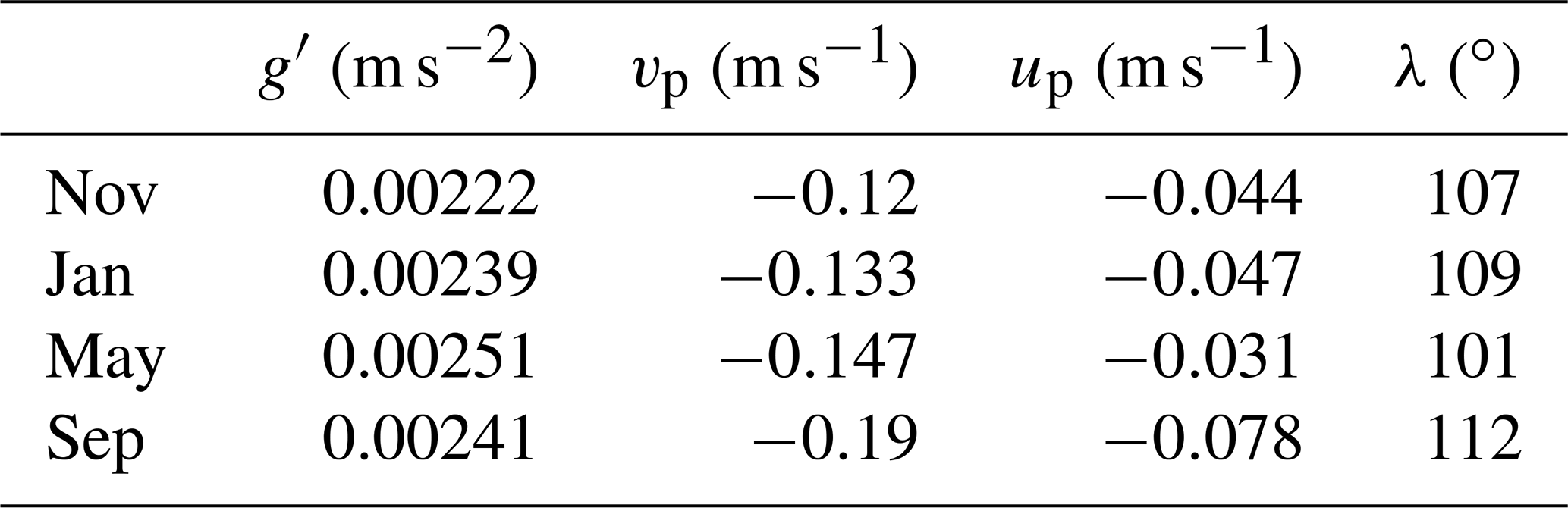
What stands out from Table 1 is that the main features of deep flow are different in each season. These differences show that the deep flow velocity and reduced gravity, g^′, fluctuate during the year, 0.127–0.2 m s⁻¹ (magnitude of the velocity components) and 0.00221–0.00251 m s⁻² (reduced gravity), respectively. As a result, λ is changeable between 101 and 112^∘. It is predicted that the flow may show varying behavior when moving over the Absheron sill and then into the southern basin. Here, we focus on how much water sinks under different initial conditions over the strait. To show this, some transects are plotted and are shown in Fig. 10. These transects are I and II (see Fig. 1b) and are used evaluate how much the water sinks after moving 20 km into the southern basin. The isopycnal 1008.9 kg m⁻³ is considered as a reference for all months for the main deep flow boundary. First and most importantly, the reference isopycnal should be close to the bottom. In addition to this, it is better to opt for an isopycnal that is clear for all months for better comparisons. It is then possible to use one method for the flow volume flux calculation for all months. Although we could have chosen 1008.95 kg m⁻³ for May and September because it is closer to the bottom, this value would have been unsuitable for November due to the fact that the maximum isopycnal is 1008.9 kg m⁻³. Thus, we chose the 1008.9 kg m⁻³ isopycnal to estimate the flow in all transects and for all months.

Transects I and II are used due to the fact that there is only a short distance between them and because the entrainment and friction effects are less on the overflow compared with some other transects, such as transect IV.

In this section, we investigate the effects of the different initial conditions on the deep flow. Based on the results shown in Fig. 10, similar isopycnals are located at depths 105 m for January and 125 m for September. These depths are the mean of the maximum and minimum depths of the reference isopycnal.

Figure 9 (a) A schematic diagram of the sinking flow in the middle basin and the overflow current over Absheron sill (top), in addition to the topography around the sill in the middle of the Caspian Sea with the chosen coordinates (bottom). (b) The balance of forces on the overflow and flow coordinates are also shown.

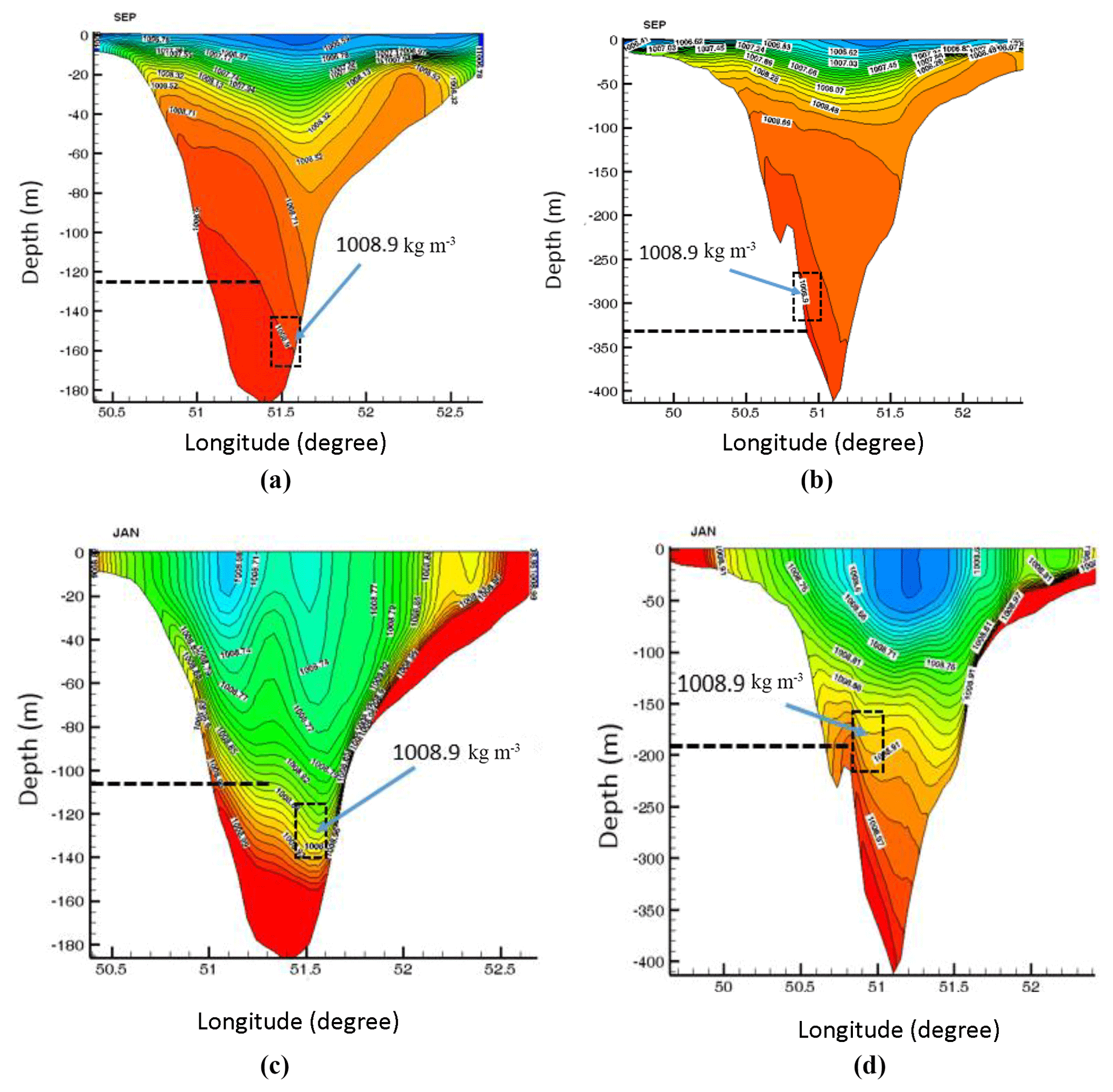
Figure 10 Simulated density fields along transects I (a, c) and II (b, d) in September (a, b) and January (c, d) 2004. The reference isopycnal of the deep flow boundary is also shown.

The results also indicate that the deep flow is confined closer to the bottom in summer than in winter. In general, the formation mechanism of the water mass can be very complex. This difficulty is related to the formation time of this water mass and how long it takes to reach the strait. To clarify this, in the previous section we mentioned that the dense flow fills the middle basin and then overflows into the southern basin (Fig. 9a). For this reason, an attempt is made to estimate the filling time in section four using some simplified assumptions. Peeters et al. (2000) estimated the filling (or flushing) time to be about 20–25 years. However, the density of water entering the southern basin is not the same in all seasons, as the water sinking processes due to evaporation and subsequent cooling in the northern basin mainly occur in winter. Nevertheless, it would be possible to track the sinking water in the strait if the numerical model simulations were for at least 20 years. The present numerical model runs are only for 5 years due to computing limitations. With a longer simulation time, it is likely that the timescales of the variability of the dense flow over the strait could be better investigated. It would also be possible to see which years the outflow is stronger or weaker (due to stronger or weaker atmospheric forcing) in, which could lead to the calculation of the filling-time range of the basins.

Despite the fact that our simulation time was shorter (5 years) than the filling time of the middle basin which is approximately 20 years (Peeters et al., 2000), the simulation results for the fifth year clearly show the overflow, but with some variability. This is due to fact that the initial conditions of the present numerical model are taken from the outputs of the HYCOM model simulations that were carried out by Kara et al. (2010); these outputs had reached a more or less steady density field, close to that of the observations, after a long period of time (about 20 years). Previous numerical simulations did not show any significant deep flow, and the simulation times were often not long enough for the basins to reach a quasi-steady state, as the main aims of such works were only concerned with the near-surface circulation processes in the Caspian Sea.

Comparison of transects I and II shows that the water sinks to depths of about 200 and 80 m in September and January, respectively, as the overflow enters the southern basin. This occurs when the water moves nearly 23 km (the distance between I and II). One of the most important reasons for this sinking depth variation may be the difference in reduced gravity that varies with season.

3 Dynamics of the overflow

The dynamics of the deep flow can be analyzed using analytical models as have been used in many other works. Among these previous studies, Girton et al. (2003) used a streamtube framework to analyze the results of their observational data in the Denmark Strait overflow. In this section, we investigate the dynamics of the overflow in the Caspian Sea. The flow, after entering in the southern basin, deflects to the right and is trapped on the western boundary of southern basin topography. In the course of this process, Coriolis, buoyancy, bottom friction and entrainment are the most important forces which affect the deep flow (Fig. 9b). A better approach would be to use a method which includes all of the forces affecting the flow dynamically. Although there are many quantities which are important in terms of the deep flow dynamics, the vorticity and potential vorticity are often used to investigate such flow behavior. Generally, vorticity is one of the most important variables in oceanography with respect to understanding the main features of the water column when moving over a strait. It is also clear that some of the main features can be shown using numerical model simulation.

As mentioned in Sect. 2, although the main aim of carrying out numerical simulations was to show the deep overflow in the Caspian Sea, the simulations also showed that after the deep overflow is trapped in the southern basin it seems to create eddies, particularly near the Iranian coast. As the deep flow reaches the Sefid Rud Cape, it separates from the coast and forms one or two eddies. Similar flow behavior has also been observed in the Persian Gulf outflow as it enters the Oman Sea. The Persian Gulf outflow can separate from the Ras Al Hamra Cape in the Oman Sea while being attached or detached from the cape depending on the outflow properties; its buoyancy varies with seasons (Ezam et al., 2010). In a flow such as this, the behavior of the vorticity and potential vorticity of the flow column upstream of the cape is linked to the separation of the flow from the cape, as previous works (Ezam et al., 2010; Stern, 1980) have shown. Here the numerical simulation outputs are used to calculate the vorticity and potential vorticity along the deep flow. Falcini and Salusti (2015) presented a method to estimate the vorticity of the water column. This formula is very useful due to the consideration od all of the forces which are important in the present overflow dynamics. Thus, this method is also used in the present work. Here, the deep flow entrainment parameter and drag coefficient are first calculated, and then the dynamic model of the deep flow is discussed.

3.1 Estimation of the drag coefficient and the entrainment parameter of the deep flow

Johnson and Sanford (1992) estimated the drag coefficient, $C_{\text{d}}=\mathrm{3}\times {\mathrm{10}}^{-\mathrm{3}}$, from the analysis of data from the Mediterranean outflow; Girton and Sanford (2003) used $C_{\text{d}}=\mathrm{3}\times {\mathrm{10}}^{-\mathrm{3}}$ for the Denmark Strait, and Cheng et al. (1999) studied the bottom roughness length and bottom shear stress in South San Francisco Bay and calculated C_d as ranging from $\mathrm{2}\times {\mathrm{10}}^{-\mathrm{3}}$ to $\mathrm{6}\times {\mathrm{10}}^{-\mathrm{3}}$. To simplify the analysis, we define $r_{\text{b}}=\frac{c_{\text{d}}U}{H}$ and $r_{\text{e}}=\frac{E}{H}$. In this study, we conducted the analysis using $C_{\text{d}}=\mathrm{3}\times {\mathrm{10}}^{-\mathrm{3}}$ and $\mathrm{5}\times {\mathrm{10}}^{-\mathrm{3}}$. Hence, r_b=C_dU/$H=\mathrm{0.003}\times \mathrm{0.2}/\mathrm{50}\sim \mathrm{1}\times {\mathrm{10}}^{-\mathrm{5}}$ s⁻¹ and r_b=C_dU/$H=\mathrm{0.005}\times \mathrm{0.2}/\mathrm{50}\sim \mathrm{2}\times {\mathrm{10}}^{-\mathrm{5}}$ s⁻¹. Here, r_b is the bottom friction parameter, U is the magnitude of the deep flow velocity, and H is the thickness of overflow. E is an entrainment speed and is defined as $E=E^{*}\times U$, where E^* is the entrainment coefficient that depends on the overflow top boundary Richardson number (Price and Bringer, 1994). Ri is the bulk Richardson number defined as $\mathit{Ri}=\frac{g^{\prime }H}{U^{\mathrm{2}}}\cos \mathit{\theta }$, where θ is the bottom slope. There are many methods of calculating the entrainment parameter, E^*, and some of these methods are presented in Table 2. Due to the importance of E^* in the next section regarding the estimation of vorticity, the E^* for transects I, II, III, IV and V is calculated based on the formulas in Table 2. Figure 11 shows E^* versus Ri for May from transects I to V.

Based on Ri for the overflow, Ri varies at different locations. Using a U value of 0.1 to 0.2 m s⁻¹, $g^{\prime }=\mathrm{0.00222}-\mathrm{0.00251}$ m s⁻², H=50–70 m, tan θ=0.02 and $\mathit{Ri}=\frac{\mathrm{0.00251}\times \mathrm{50}}{\mathrm{0.2}\times \mathrm{0.2}}\mathrm{0.99}\sim \mathrm{3.1}$. Based on Table 2 with $\mathit{Ri}>=\mathrm{0.8}$, we used a mean E^* value based on Eqs. (2), (3), (4) and (5) (equations from Table 2), because we cannot use the formula $\mathrm{1}(\mathit{Ri}>=\mathrm{0.8}$, then $E^{*}<=\mathrm{0}$). For this section, r_e, the entrainment parameter, values are considered to be $\mathrm{5}\times {\mathrm{10}}^{-\mathrm{6}}$ and $\mathrm{1}\times {\mathrm{10}}^{-\mathrm{5}}$ s⁻¹ based on typical values for Ri, U and H.

Table 2 Some of the published E^* equations based on Ri (Kashefipour et al., 2010).

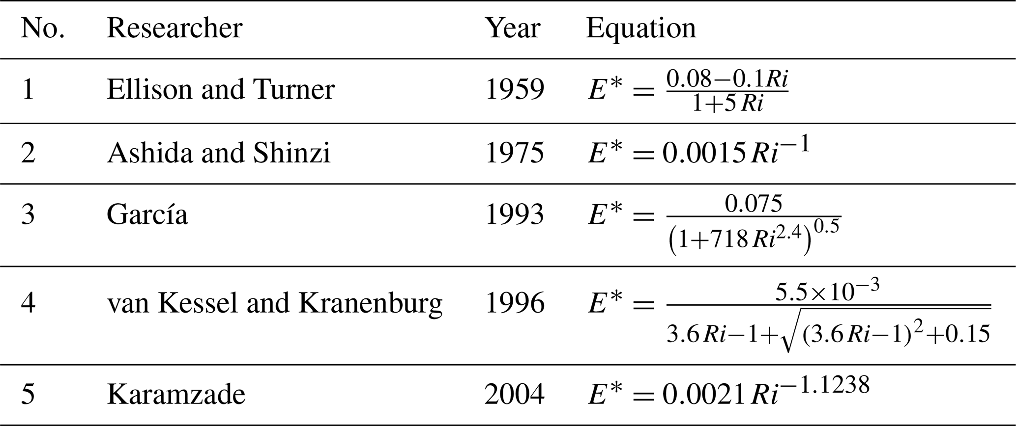
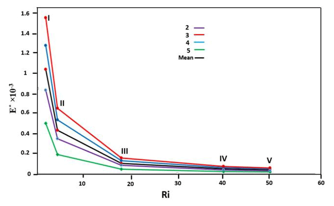
Figure 11 Changes of entrainment coefficients based on different Richardson numbers for May in the transects shown in Fig. 1b. The formulas in Table 2 are used to estimate E^* (the numbers refer to the equation numbers in Table 2). To use E^* in Eqs. (1) and (2) (Sect. 3.2), the mean values for E^* is also estimated (black).

3.2 The changes of vorticity and potential vorticity of the overflow

As previously mentioned , vorticity is an important parameter for the study the column properties of overflow over the sill. Furthermore, the vorticity can be useful to consider the behavior of the flow (e.g., Stern, 1980) in the southern basin, particularly near the Sefid Rud Cape. Not only do we try to estimate the vorticity of the water column and the width of the flow as it moves into the southern basin, especially during the adjustment of the flow width, but we also attempt to estimate the flow vorticity and its behavior near the cape. The width of the flow is calculated directly from the numerical simulations; however, for the calculations of vorticity and PV (potential vorticity) we need to use an analytical model.

Here we consider the structure of the flow as it moves over the sill in terms of its vorticity and PV. Falcini and Salusti (2015) presented an analytical model for the Sicilian Channel: the vorticity and PV equations are based on the streamtube model (Smith, 1975; Killworth, 1977). To deal with this, they used a (ξ, ψ) coordinate system, which was a modified form of the system used by Astraldi et al. (2001). In this frame, ξ is the along-flow coordinate and ψ is the cross-flow coordinate (see Fig. 1 in Smith, 1975). Using this method, friction and mixing effects are considered in the estimation of potential vorticity. Firstly, Falcini and Salusti (2015) used the hydrostatic pressure equations for three layers to achieve equations for entrainment and friction; next, they concentrated on the third layer (with dense water near the bottom) to obtain formulas for vorticity and potential vorticity. In addition to this, based on their assumptions (Falcini and Salusti, 2015), the velocity of a streamline is a function of ξ only. They defined β as the angle between the (ξ, ψ) and (x, y) coordinates, and assumed that β is close to zero in the channel. They then used the classical vorticity equation (Gill, 1984) and assumed cross-sectional averages of the various terms in the steady state of the vorticity equation due to the difficulty of depth and velocity calculations at different positions from hydrographic data. They presented Eqs. (1) and (2) to calculate vorticity and potential vorticity for dense flow (the deepest moving layer). These formulas are based on a homogeneous bottom water vein while using shallow water theory (over bars indicate cross-sectional averages). To obtain a formula, the bottom water is assumed to be well mixed and the flow has a strong axial velocity, which is nearly uniform over the cross section of the stream; furthermore, the cross-stream scale is assumed to be much smaller than the local radius of curvature of the streamline axis. Relative vorticity and potential vorticity distributions of the deep flow are as follows:

$$\begin{array}{}\text{(1)}& {\displaystyle }& {\displaystyle \frac{\stackrel{\mathrm{‾}}{\mathit{\zeta }}}{f}}={\displaystyle \frac{{\stackrel{\mathrm{‾}}{u}}_{\mathrm{0}}}{\stackrel{\mathrm{‾}}{u}}}{e}^{-{\int }_{\mathrm{0}}^{\mathit{\xi }}\frac{r_{\text{b}}}{u}\text{d}x}\left({\displaystyle \frac{\stackrel{\mathrm{‾}}{{\mathit{\zeta }}_{\mathrm{0}}}}{f}}+{\displaystyle \frac{\mathrm{1}}{\stackrel{\mathrm{‾}}{u_{\mathrm{0}}}}}\underset{\mathrm{0}}{\overset{\mathit{\xi }}{\int }}{e}^{{\int }_{\mathrm{0}}^x\frac{r_{\text{b}}}{u}\text{d}\stackrel{\mathrm{´}}{x}}\left[{\displaystyle \frac{\stackrel{\mathrm{‾}}{u}}{\stackrel{\mathrm{‾}}{h}}}\stackrel{\mathrm{‾}}{{\displaystyle \frac{\partial h}{\partial x}}}-{\displaystyle \frac{E}{\stackrel{\mathrm{‾}}{h}}}\right]\text{d}x\right)\text{(2)}& {\displaystyle }& {\displaystyle }\mathrm{\Pi }=e^{-{\int }_{\mathrm{0}}^{\mathit{\xi }}\frac{\mathrm{\Gamma }}{u}\text{d}x}\left[{\mathrm{\Pi }}_{\mathrm{0}}-\underset{\mathrm{0}}{\overset{\mathit{\xi }}{\int }}{e}^{{\int }_{\mathrm{0}}^x\frac{\mathrm{\Gamma }}{u}\mathrm{d}\stackrel{\mathrm{´}}{x}}{\displaystyle \frac{r_{\mathrm{b}}\mathit{\zeta }}{hu}}\text{d}x\right],\end{array}$$

where $\mathrm{\Gamma }=\frac{E}{h}$.

To obtain Eq. (1), it is supposed that $\stackrel{\mathrm{‾}}{{\mathit{\zeta }}_{\mathrm{0}}}\ll f$. After integrating the shallow-water equations along the flow and mass continuity equation and using some mathematical operations, Eqs. (1) and (2) are obtained.

Here ζ and Π are the mean relative vorticity and potential vorticity, respectively, h is the layer thickness, $\partial h/\partial x$ represents the slopes of the flow reference isopycnals, and ζ₀ and $\stackrel{\mathrm{‾}}{u_{\mathrm{0}}}$ are the initial vorticity and velocity, respectively. ζ₀ is estimated as U∕W, where U and W are the flow speed (∼0.2 m s⁻¹) on the sill and the cross channel scale (∼20 km) over the sill, respectively. To be applicable, some terms in Eq. (1) are considered as cross-sectional averages. Three terms are significant in vorticity: the stretching term, the entrainment effect and the friction. To estimate all parameters in these formulas, we use five transects from the strait (I) to the southern area (V) (Fig. 1b). Typically, for November in transect III, $\partial h/\partial x\approx \mathrm{0.0047}$ (δh∼180 m and δx∼38 km), $\stackrel{\mathrm{‾}}{u}=\mathrm{0.11}$ m s⁻¹ and $\stackrel{\mathrm{‾}}{h}=\mathrm{180}$ m are estimated. The calculations of r_b and r_e are based on the Ri number (presented in Sect. 3.1 and the formulas in Table 1). Thus, $r_{\text{b}}=\mathrm{2}\times {\mathrm{10}}^{-\mathrm{5}}$ (s⁻¹) and $r_{\text{e}}=\mathrm{4}\times {\mathrm{10}}^{-\mathrm{6}}$ (for transect II) and $\mathrm{8}\times {\mathrm{10}}^{-\mathrm{7}}$(for transect III) are calculated based on Fig. 11. In transect IV and V, r_e∼0 because of large Ri ∼ 40 to 50. Using Eqs. (1) and (2), profiles of ζ and Π are plotted in Fig. 12 as functions of ξ along the streamtube.

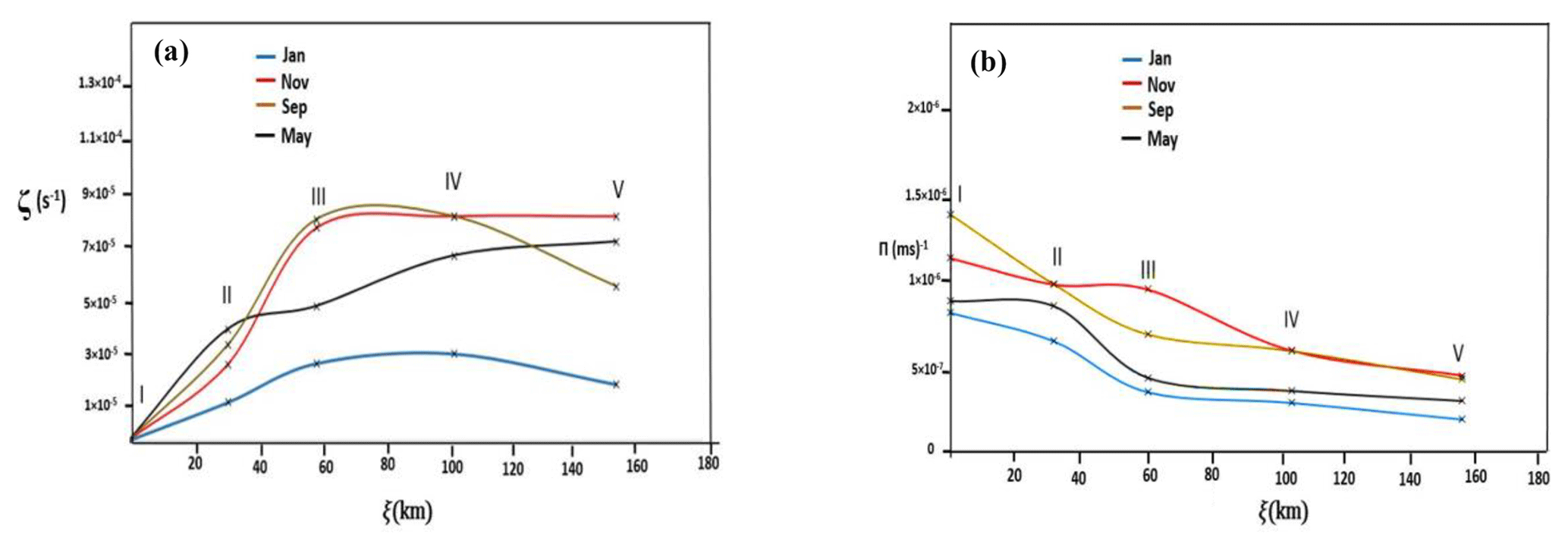
Figure 12 Changes in ζ (s⁻¹) (a) and Π (m⁻¹ s⁻¹) (b) along the flow based on Eqs.(1) and (2).

Figure 12 shows that ζ increases from transects I to V, due to of the stretching term in Eq. (1), although the September and January values have different behaviors in transects IV to V. However, after transect III, the changes are not considered, because the depth does not vary significantly (stretching term) and entrainment has been ignored as the Ri number is large after this transect. In the month of November, the vorticity has a maximum value of about $\mathrm{8.5}\times {\mathrm{10}}^{-\mathrm{5}}$ (s⁻¹) in transect V, although in January the vorticity value is the lowest among all of the months shown. When it comes to Π, the graph shows a decrease in PV values along the flow from I to IV, but after IV, the Π values are almost constant. For example, changes of Π over the sill (from I to III) are about $\mathrm{7}\times {\mathrm{10}}^{-\mathrm{7}}$ (m⁻¹ s⁻¹) and $\mathrm{4}\times {\mathrm{10}}^{-\mathrm{7}}$ (m⁻¹ s⁻¹) for September and January, respectively, due to bottom friction and entrainment.

Transects I, II and III are located on the slope and IV and V are in deeper parts of the southern basin. The vorticity and PV values are based on the topography of the Caspian Sea. Figure 12 shows that the changes of vorticity are more marked from I to III because the depth of the flow changes more on the slope (stretching term) over this distance. As the flow enters the southern Caspian Sea basin, it adjusts into an internal quasi-geostrophic flow, almost like a deep western boundary current in the southern Caspian Sea basin. The gravity-driven flow appears as a trapped current after the Absheron sill due to the Coriolis effect (transects IV and V). When moving along the southern (Iranian) coast, the forces of the pressure gradient and the Coriolis effect balance the force of friction. The entrainment effect can be ignored because the Richardson number is about 50 in transect V based on Fig. 11, so $E^{*}\sim \mathrm{0}$. The width of the flow over the sill and when it is trapped is calculated for all months (from the numerical simulation results) and varies for various seasons; here it is shown for transect V. These values are 18, 16, 34 and 35 km for November, January, May, and September, respectively. As Fig. 12 shows, the potential vorticity of the water column decreases from transects I to V due to frictional and entrainment effects. The comparison of the flow width from transects I to V also shows that the bottom friction (and the entrainment, particularly over the strait) increases the width of the flow in the southern basin. For example, for September, the width of the flow increases from 20 km (I) to 35 km (V), by about 15 km, as a result of moving over the sill and into the southern basin. This means that the friction force decreases the potential vorticity of the flow in the southern basin.

Apart from this, the trapped current continues moving into the western part of the southern basin (Fig. 13), but it shows an interesting behavior as it reaches the Sefid Rud Cape. The flow separates from the cape and forms one or two eddies (Fig. 14). Based on the numerical results, the separation of the dense flow from the cape depends on the season (different boundary currents for different seasons). The most important parameter determining the behavior of flow when it separates from the cape is its potential vorticity.

In this section, the potential vorticity of the deep flow is estimated for different seasons based on certain information, as in Fig. 14. We observe different behavior of the flow when separating from the cape for fall in November and in spring (May; Fig. 14). For example, in transect V for November and May, the values of the potential vorticity are $\mathrm{6}\times {\mathrm{10}}^{-\mathrm{7}}$ and $\mathrm{4}\times {\mathrm{10}}^{-\mathrm{7}}$ (m s)⁻¹, respectively (Fig. 12). Figure 14 indicates that in November, the flow is closer to the cape than in May during the time of separation. Therefore, it can probably be concluded that the potential vorticity upstream of the flow can affect the flow when it separates from the cape, although other factors, such as the Rossby number, are also important. In order to be more accurate, Stern (1980) showed that for this kind of the flow with a zero potential vorticity assumption, the flow separates from the cape when the width of the flow upstream of the cape is less than about 0.42 R_D, where R_D is the Rossby radius of deformation $R_{\text{D}}=(g^{\prime }H{)}^{\mathrm{0.5}}/f$ (based on the current depth, H, and its reduced gravity, g^′, far upstream). Based on Fig. 12, we can still use the Stern method for this flow, although the potential vorticity is not quite zero upstream of the cape (Fig. 12b). Based on typical values of the R_D∼2L, which is about 30 km, and the width of the western boundary current (about 15 to 35 km, calculated above) which is of the same order as 0.42R_D, the flow may just be separated from the cape, especially in January and November (with respective widths of 16 and 18 km). Figure 14 indicates that separation and formation of a cyclonic mesoscale eddy near the cape are more pronounced in November. Considering the fact that the PV of the flow is not quite zero before the cape, the Stern criteria may not apply for such flow separation. A more rigorous criterion is needed for the separation of such flow from the cape that may also be dependent on the geometrical dimensions of the cape.

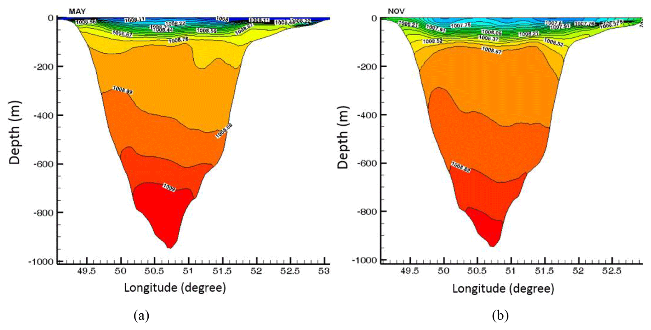
Figure 13 Density fields along transect V (from the numerical model) in May (a) and November (b).

Figure 14 Monthly mean currents (m s⁻¹) in the layer “k=11”, obtained from the model simulations for May (a) and November (b). The dense flow separates from the Sefid Rud Cape. The bottom deep, topographically trapped current over the Absheron sill and the southern Caspian Sea basin is marked. k=1 is the bottom layer and k=30 is the top layer.

4 Flushing time and the importance of this work

4.1 Volumes of basins' dense water and flushing time calculations

As mentioned in Sect. 2 and discussed in the following section, the flushing times of the Caspian Sea basins are important parameters for this ecosystem. To calculate the basin flushing time, the first and most important step is the estimation of the dense flow volume flux when entering the southern basin over the Absheron sill. A simple method to calculate the deep flow volume flux is multiplying the mean velocity of the overflow by its cross section (Eq. 3). Although the numerical model outputs directly give the velocity, the cross section should be calculated. Here the deep flow volume flux is also estimated by Eqs. (3)–(6), in addition to deep flow volume flux obtained by the numerical simulations.

It is very useful to use an equation which is compatible with the physical conditions of the Absheron sill. For this reason, the shape of the sill and the deep flow reference isopycnal are considered when obtaining an appropriate Eq. (6) for the deep flow volume flux. Here the accuracy of this formula is checked using the numerical simulation results. Although the use of observational data is common for deep flow volume flux estimation, we do not have ADCP data across the Absheron sill. Hence, here we try to obtain a formula using temperature and salinity data that are much more available than the ADCP data in the study region.

The overflow volume flux is given by Eq. (3) in which v is the mean magnitude of the geostrophic velocity of the overflow and ds is an element of its cross-sectional area:

$$\begin{array}{}\text{(3)}& Q_{\text{v}}=\int v\text{d}s\end{array}$$

Due to the parabolic form of the bottom topography (Z) of the Absheron Strait, its geometry and the upper surface of the dense overflow in this valley-like shape (Fig. 15a, b) can be given by

$$\begin{array}{}\text{(4)}& z=a{x}^{\mathrm{2}}+bx+c,h^{\prime }=A{e}^{-ax},\end{array}$$

where a, b, c, A and α are assumed to be constant and we also assign the deep flow reference isopycnal depth (approximately the top boundary of the overflow) as h^′ (see Fig. 15b).

Due to the fact that Z and h^′ (deep flow isopycnal reference line) in the graph (Fig. 15a, b) are from L₁ to L₂, we can calculate h^′ and Z values at (x=L₁) and (x=L₂). Substituting Eq. (4) into Eq. (3) and using the assumptions that v is the mean deep flow geostrophic speed, is constant (in each month and uniform in depth) and is given by the slope of h^′ in the x direction, we have

$$\begin{array}{ll}\text{(5)}& {\displaystyle }{Q}_{\text{v}}=& {\displaystyle }{\displaystyle \frac{g^{\prime }}{f}}{\displaystyle \frac{H_{\mathrm{1}}-H_{\mathrm{2}}}{\left|L_{\mathrm{2}}\right|+\left|L_{\mathrm{1}}\right|}}\left[\left(-{\displaystyle \frac{A}{\mathit{\alpha }}}{e}^{-\mathit{\alpha }{L}_{\mathrm{2}}}-e^{\mathit{\alpha }{L}_{\mathrm{1}}}\right)\right.{\displaystyle }& {\displaystyle }\left.-{\displaystyle \frac{a}{\mathrm{3}}}\left(L_{\mathrm{2}}^{\mathrm{3}}+L_{\mathrm{1}}^{\mathrm{3}}\right)-{\displaystyle \frac{b}{\mathrm{2}}}\left(L_{\mathrm{2}}^{\mathrm{2}}-L_{\mathrm{1}}^{\mathrm{2}}\right)\right],\end{array}$$

where

$$a={\displaystyle \frac{H_{\mathrm{2}}{L}_{\mathrm{1}}+H_{\mathrm{1}}{L}_{\mathrm{2}}}{L_{\mathrm{1}}(L_{\mathrm{2}}^{\mathrm{2}}+L_{\mathrm{1}}{L}_{\mathrm{2}})}}$$

$$b={\displaystyle \frac{H_{\mathrm{2}}{L}_{\mathrm{1}}+H_{\mathrm{1}}{L}_{\mathrm{2}}}{L_{\mathrm{2}}^{\mathrm{2}}+L_{\mathrm{1}}{L}_{\mathrm{2}}}}-{\displaystyle \frac{H_{\mathrm{1}}}{L_{\mathrm{1}}}}$$

If we assume that $L=\frac{\left|L_{\mathrm{1}}\right|+\left|L_{\mathrm{2}}\right|}{\mathrm{2}}$, we have

$$\begin{array}{}\text{(6)}& Q_{\text{v}}={\displaystyle \frac{g^{\prime }}{f}}{\displaystyle \frac{H_{\mathrm{1}}-H_{\mathrm{2}}}{\left|L_{\mathrm{2}}\right|+\left|L_{\mathrm{1}}\right|}}\left[{\displaystyle \frac{\mathrm{2}A}{\mathit{\alpha }}}\sin h\left(\mathit{\alpha }L\right)-{\displaystyle \frac{\mathrm{2}}{\mathrm{3}}}a{L}^{\mathrm{3}}\right],\end{array}$$

where

$$a={\displaystyle \frac{H_{\mathrm{2}}+H_{\mathrm{1}}}{\mathrm{2}{L}^{\mathrm{2}}}}$$

$$b={\displaystyle \frac{H_{\mathrm{2}}-H_{\mathrm{1}}}{\mathrm{2}L}}$$

$$A={\displaystyle \frac{H_{\mathrm{1}}}{e^{aL}}}$$

$$a={\displaystyle \frac{-\mathrm{1}}{\mathrm{2}L}}Ln{\displaystyle \frac{H_{\mathrm{2}}}{H_{\mathrm{1}}}}$$

To obtain Eq. 6, which is an approximation for $\left|L_{\mathrm{1}}\right|=\left|L_{\mathrm{2}}\right|$, we defined L based on L₁ and L₂. Although the minimum of Z is not exactly at x=0, it does not create a large error. To show this in reality, the Q_v is calculated separately using Eqs. (5) and (6). The results show that the difference is about 2 %–5 % when using (Eq. 5) without any assumptions ($L\sim \left|L_{\mathrm{1}}\right|\sim \left|L_{\mathrm{2}}\right|$). Another important point is that the geostrophic balance between v and h^′ is assumed to be R_o∼0.1 based on the flow parameter estimations of Sect. 2.

To calculate the mean monthly volume flow rate of the deep current that enters the southern basin of the Caspian Sea, we assume that its density is greater than 1008.78 kg m⁻³. The average density (for different seasons) of the flow below the deep flow upper boundary (e.g., Fig. 15), are then used to calculate the deep flow volume flux, Eq. (6) and Fig. 15.

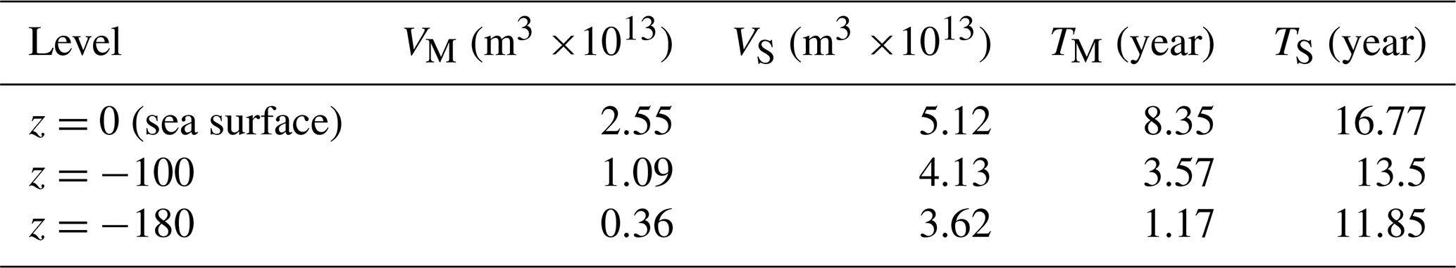
For the times that the middle and southern basins are filled, first the volumes of the middle (V_M) and southern (V_S) basins (see Fig. 15c) are calculated below three levels: z=0, $z=-\mathrm{100}$ and $z=-\mathrm{180}$ m ($z=-\mathrm{180}$ m is the approximate depth of the Absheron sill, and would be more appropriate for the southern basin). Then, if we assume a similar annual mean value of Q_v for both basins, these filling times are estimated. The results of these calculations and comparisons between them for different seasons are given in Tables 3 and 4. The results show that the maximum and minimum flow rates of abyssal water that enter the southern Caspian Sea are in May and November, respectively. In order to check the accuracy of Eq. (6), the Q_v is also directly calculated from the numerical simulations without any assumptions. As shown in Table 3, the numerical model value is greater than that of the analytical estimation. This underestimation by Eq. (6) could be due to the fact that we used certain assumptions to obtain Eq. (6). The velocity used is the geostrophic velocity and the deep flow isopycnal reference lines are also simplified. In addition, some errors stem from the choice of the 1008.78 kg m⁻³ contour, as its position changes for different months (see Sect. 2.3). To solve this problem, we utilize one method for all months (using the same boundary conditions for all months), to acquire approximate estimates. The flushing times are then estimated based on the direct calculation from the numerical simulations. The results show that the flushing times are about 6–7 years (middle basin) and 13–15 years (southern basin) for the numerical simulations based on z=0, which are similar results to those from Eq. (6) (Table 4).

Equation (6) could also be useful for the estimation of the volume flux of overflows in other straits, particularly in oceanic contexts without ADCP data, such as in the Persian Gulf where there are many CTD data in the Hormuz Strait (Bidokhti and Ezam, 2009).

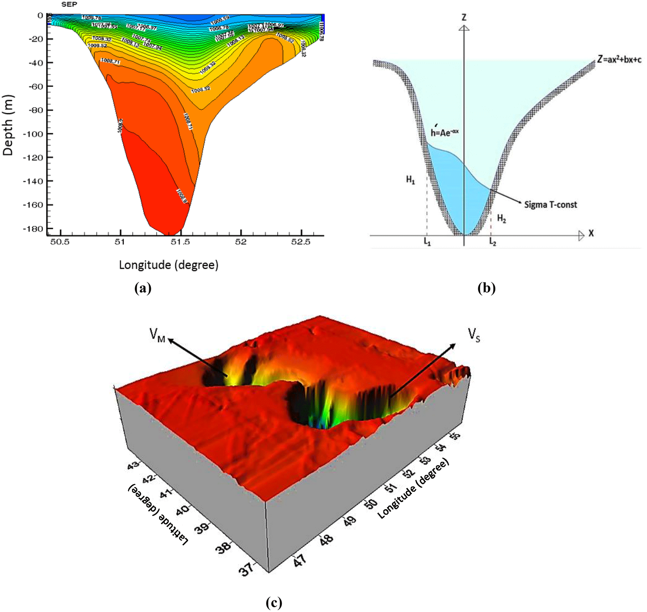
Figure 15 (a) Typical density fields along transect I for September from which we calculate the flow rates. (b) The scheme of the topography with a typical isopycnal and model parameters. (c) The model bathymetry used to calculate the volumes of the middle (V_M) and southern (V_S) basins. The Surfer software is used to plot and calculate V_M and V_S using GEBCO data with a ${\mathrm{0.5}}^{\circ }\times {\mathrm{0.5}}^{\circ }$ resolution.

Table 3 The model deep flow boundary current parameters (1Sv=10⁶ m³ s⁻¹) for different months. The last column shows direct calculations from the numerical model.

Table 4 Flushing times of the middle (T_M) and the southern (T_S) basins (using an annual average volume flow rate, Q_V, below three levels based on Eq. 6).

4.2 The importance of deep flow in the southern basin

In Sect. 4.1, we estimate the Caspian Sea basins' flushing times because they are very important for the ventilation of these deep basins. In addition to this, in Sect. 2, it was discussed why this timescale is important for the required time of the numerical simulations of the Caspian Sea, particularly for the proper adjustment of the deep regions. In this section, the importance of other aspects of the deep flow are discussed. In general, deep flows play a pivotal role in the water ventilation of deeper parts of the Caspian Sea. Signs of life are observed in the deep region of the Caspian Sea, especially in the southern basin (Terziev, 1992); however, the reasons for the existence of marine life have not been clearly addressed to date. The main reason that the deeper part of the southern Caspian Sea basin is not “dead” like that of the Black Sea is that oxygen is carried from the surface layers to the bottom layers, and nutrients are moved from the bottom layers towards the top layers by a slow advection. As a result of this, the Absheron sill overflow can be considered as the most important element of this ecosystem in the southern basin of the Caspian Sea. Moreover, these days, oil well pollution and climate change effects are the biggest issues in the Caspian Sea. Particularly, it is interesting to note the locations of the oil and gas wells in this sea (the location of the oil and gas wells in the basin are shown in figure 16a). It can be seen that they are mainly situated in two areas in the northern basin and particularly around Absheron sill (at present). Furthermore, satellite imagery shows that some oil spills have occurred in the vicinity of the oil and gas wells around the sill. For example, Fig. 16b, which is extracted from Marina and Lavrova (2015) using satellite data, shows that the spills are located on the sill and also in the western parts of the southern basin. In addition to this, studies on the sea bed in the Absheron Strait and the Bako Gulf both have found approximately 1 and 1.5 m of sludge and oil residues in the form of high-density pellets and mazut (Escani and Amini, 2013). If we consider all of these points and look at the path of the deep flow (Fig. 14), the present work may be very important regarding the impacts of oil exploration activities with respect to the fate of the deeper (as well as other depths) reaches of this environment – particularly if certain careful action is not taken.

Based on the discussion so far, the existence of deep flow on the sinking and mixing processes is very important with respect to the ventilation of the southern basin. Unfortunately, oil pollution can spread into the deeper reaches of the southern basin via this deep flow. In other words, this deep flow plays a positive role in the ventilation of the deeper parts of the Caspian Sea, but due to the oil exploration activities at the bottom of this enclosed sea, this deep flow can also have a negative effect on the region via the transport of polluted materials.

The overflow direction was calculated and showed that the flow passes over some oil drill holes on Absheron sill. Due to the angle, the flow passes over wells near the Azerbaijani Republic rather than the eastern part of the sill near Turkmenistan. In Sect. 3, the dynamics of the flow were discussed. Among all of the aspects involved with the dynamics, it was found that under certain conditions the flow was separated from the Sefid Rud Cape (based on Sect. 3.2) and two eddies were formed in this region. Eddies are very significant in the ocean (Gill, 1984) because they advect mass (in this case, oil pollution or even harmful algae blooms) and their ability to propagate is crucial to their contribution to marine mixing (Flierl, 1987). Based on the path of the deep flow and the eddy formation near Sefid Rud Cape, it can be concluded that the region near the Sefid Rud Cape may currently be home to the most polluted waters in the deeper reaches, and that pollution can spread other deeper parts of the southern basin of the Caspian Sea (Fig. 16b).

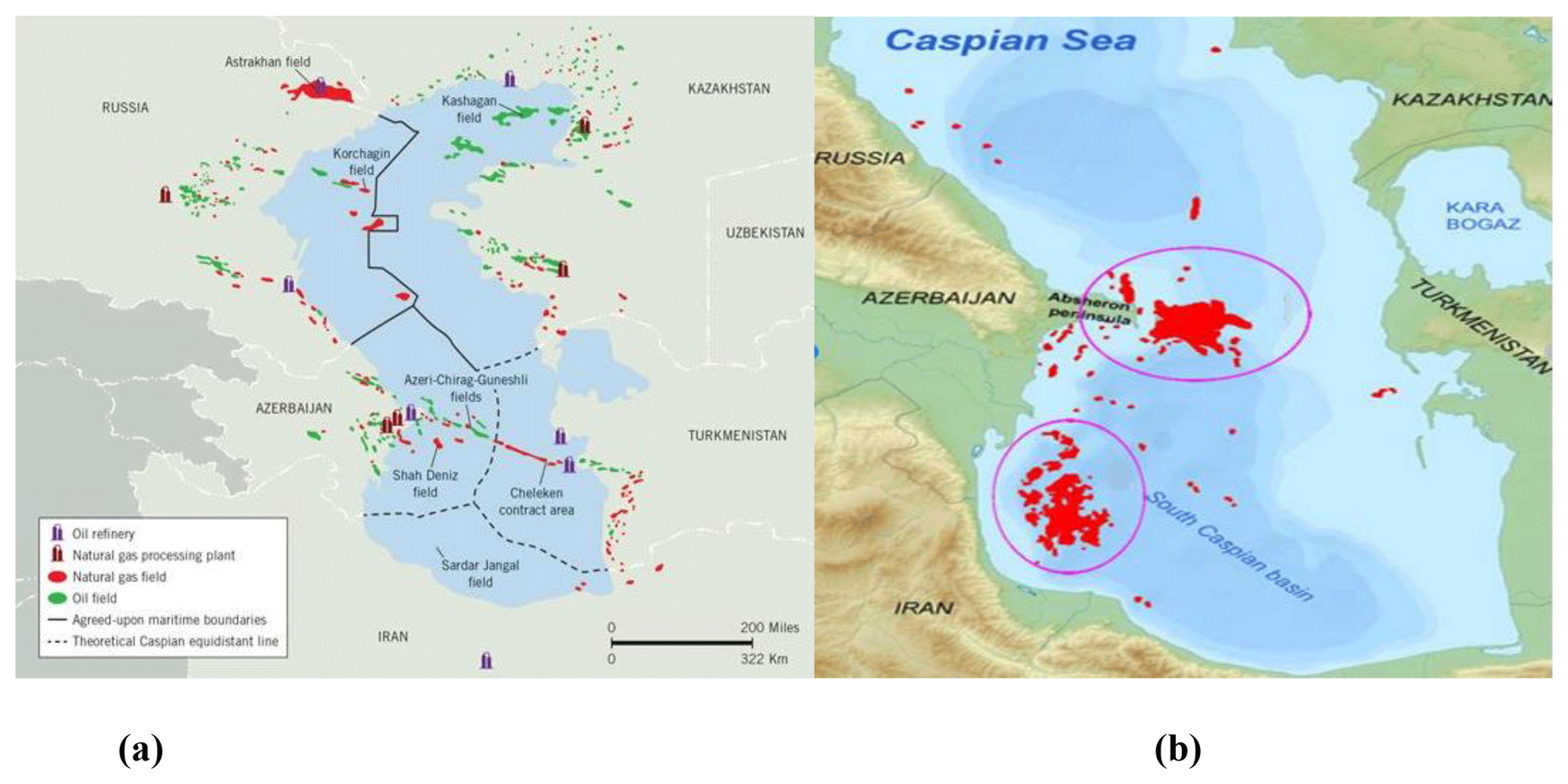
Figure 16 (a) The locations of oil and gas fields in the Caspian Sea, extracted from https://www.offshore-mag.com (last access: 11 September 2013). (b) A map of oil spills revealed from satellite radar imagery in the central and southwestern parts of the Caspian Sea in 2010 (Mityagina and Lavrova, 2015).

These days, climate change is has led to many problems in this area, like sea level rise (Chen et al., 2017), mainly due to the trend of increasing atmospheric temperature in recent years. Due to this problem, a question has been raised regarding the effect of climate change on the deeper flows of the Caspian Sea. At present the water sinks in the northern basin and after filling the middle basin it finally overflows into the southern basin. If the atmospheric temperature continues to rise, it will warm the northern part of the Caspian Sea; hence, it is predicted that the sinking process will be weaker. As a result, the volume of water in the deep overflow will decrease and flushing time will increase. In other words, warming will probably have a negative effect on the deep part of the southern basin of the Caspian Sea due to weaker ventilation by the abovementioned deep flow, if it does not cause ventilation to cease completely.

5 Conclusions and consequences

The results of observations and numerical simulations showed that there is an abyssal flow from the middle to the southern basins of the Caspian Sea. The density difference between the deeper water of the middle basin and that of southern basin leads to an overflow gravity current over the Absheron sill. This difference is mainly due to the temperature difference between deeper parts of these two basins; winter storms and cold wind provide the cooling of this rather high-latitude shallow water in the northern basin. As a result, cold water initially sinks in the northern part of this sea (at about 48^∘ latitude), fills the middle basin and then overflows towards the southern basin. In autumn and winter, surface water cools and its density is increased; it then sinks to the deeper parts of the middle basin, which is similar to deep convection in high-latitude oceans.

We estimated typical mass transport and flushing times of the deep-water basins of this sea using the overflow properties at the Absheron sill. After the sill, the overflow adjusts itself moving south as a gravity-driven topographically trapped current, spiraling into deeper reaches due to bottom friction and entrainment. It always tends to move toward the western shores of the sea, mainly due to the Coriolis force that shifts it to the right. Such flow is important in the abyssal circulation and ventilation of the deep southern basin of the Caspian Sea. For vorticity and potential vorticity of the flow, the formulas which are presented by Falcini and Salusti (2015) are used to estimate the changes in the relative vorticity and the potential vorticity of the trapped current over Absheron sill. Results also showed that nearly 3.05×10¹² m³ of water per year can enter the southern basin via this abyssal flow, giving a typical flushing time of about 15–20 years, which is of the same order as those estimated by Peeters et al. (2000). Some points are discussed regarding how the southern Caspian Sea basin ecosystem may be strongly dependent on this flow.

The northern and middle Caspian Sea basins have become important areas with respect to oil and gas exploration (especially the shallow Absheron Strait area) and marine transport. As the Caspian Sea is an enclosed sea, the adverse effects of such activities may particularly affect the deeper parts of the sea's basins. For this reason, it is recommended that more detailed observational data are collected in the deep regions of the southern and middle basins of the Caspian Sea via joint projects with neighboring countries. More extensive and fine-resolution observational data and numerical simulations are required to uncover more details regarding the overflow structure over and around the Absheron sill (Absheron Strait) and the deeper parts of the Caspian Sea basins.