the Creative Commons Attribution 4.0 License.
the Creative Commons Attribution 4.0 License.
 | 16 Dec 2019
Non-linear aspects of the tidal dynamics in the Sylt-Rømø Bight, south-eastern North Sea
Alexey Androsov
Lasse Sander
Ivan Kuznetsov
Felipe Amorim
H. Christian Hass
Karen H. Wiltshire
This study is dedicated to the tidal dynamics in the Sylt-Rømø Bight with a focus on the non-linear processes. The FESOM-C model was used as the numerical tool, which works with triangular, rectangular or mixed grids and is equipped with a wetting/drying option. As the model's success at resolving currents largely depends on the quality of the bathymetric data, we have created a new bathymetric map for an area based on recent studies of Lister Deep, Lister Ley, Højer Deep and Rømø Deep. This new bathymetric product made it feasible to work with high-resolution grids (up to 2 m in the wetting/drying zone). As a result, we were able to study the tidal energy transformation and the role of higher harmonics in the domain in detail. For the first time, the tidal ellipses, maximum tidally induced velocities, energy fluxes and residual circulation maps were constructed and analysed for the entire bight. Additionally, tidal asymmetry maps were introduced and constructed. The full analysis was performed on two grids with different structures and showed a convergence of the results as well as fulfilment of the energy balance. A great deal of attention has been paid to the selection of open-boundary conditions, model validation against tide gauges and recent in situ current data. The tidal residual circulation and asymmetric tidal cycles largely define the circulation pattern, transport and accumulation of sediment, and the distribution of bedforms in the bight; therefore, the results presented in the article are necessary and useful benchmarks for further studies in the area, including baroclinic and sediment dynamics investigations.
- Article
(12713 KB) - Full-text XML
- BibTeX
- EndNote


The Sylt-Rømø Bight (SRB) is one of the largest tidal catchments in the Wadden Sea, which stretches from the Dutch island of Texel to Skallingen, a peninsula in Denmark. The SRB is characterized by the barrier islands Sylt (Germany) and Rømø (Denmark), which are separated by a tidal inlet called Lister Deep. Two artificial causeways, the Hindenburg Damm (1927) and the Rømøvej (1948), connect the islands Sylt and Rømø to the mainland and create a semi-enclosed back-barrier environment. Water exchange with the North Sea takes place through the 2.8 km wide Lister Deep. The main channels draining the tidal back-barrier environment are called Lister Ley, Højer Deep and Rømø Deep (Fig. 1).
The bight is characterized by large intertidal areas occupying about 40 % of the entire bight. The domain of interest has an average water depth of ∼4 m and a maximum water depth of ∼37 m in Lister Deep (Fig. 1). The tidal range in the area is ∼1.8 m (e.g. Pejrup et al., 1997) and the water column is generally well mixed (e.g. Ruiz-Villarreal et al., 2005). The annual mean freshwater discharge into the bay is only ∼7 m3 s−1 (e.g. Purkiani et al., 2015).
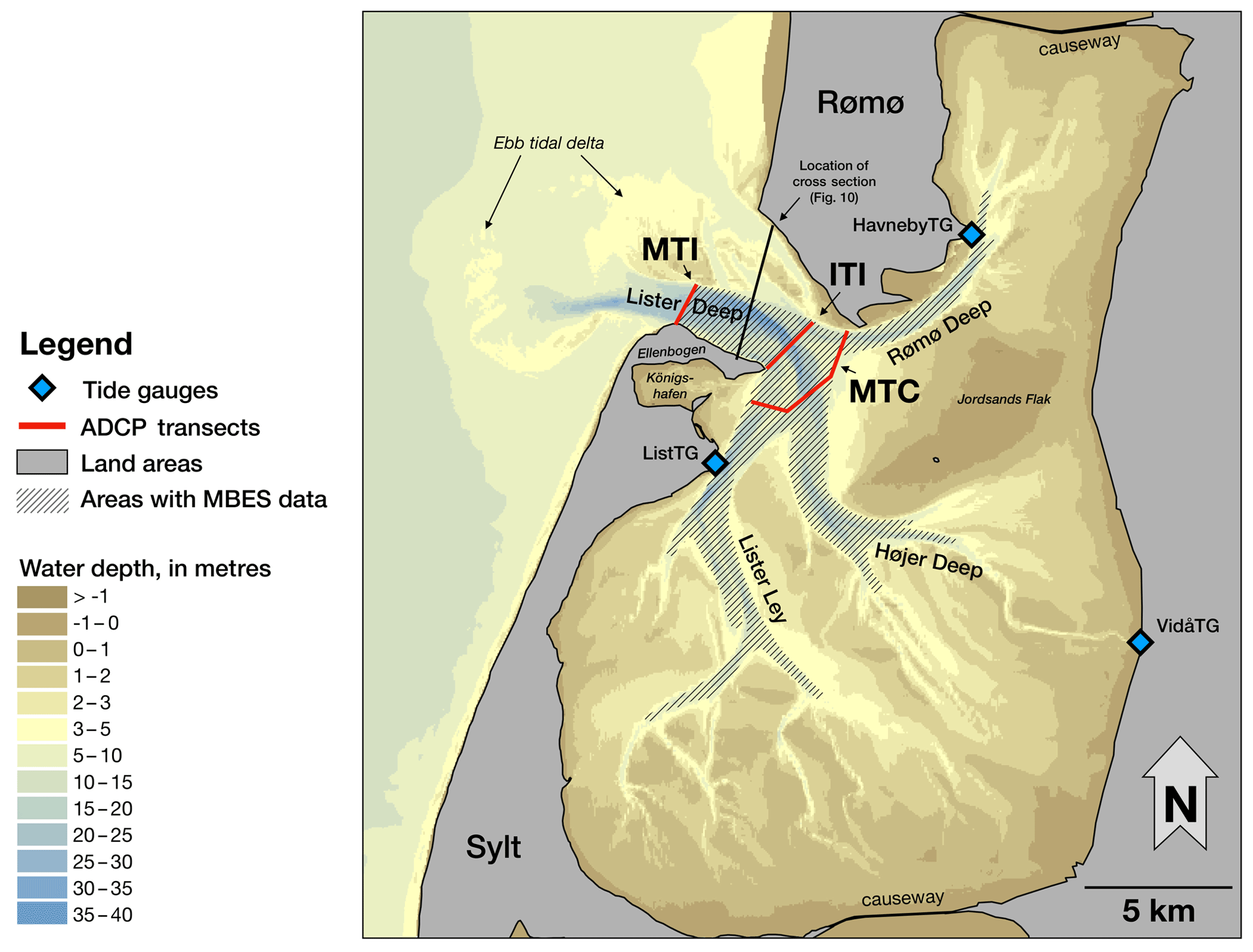
Figure 1The bathymetry of the considered domain. The red lines indicate acoustic Doppler current profiler (ADCP) transects, the blue rhombuses show positions of the tide gauges. The hatching represents the zone with the recent multibeam echo sounder (MBES) data.
The tides play a major role in the local bight dynamics. Estimates of maximum horizontal tidal velocities in Lister Deep vary from 1.2 to 2 m s−1. Estimates of the mean water volume entering the basin during flood and leaving during ebb (the tidal prism) vary from 4×10⁸ to 6.3×10⁸ m3 (Bolaños-Sanchez et al., 2005; Gätje and Reise, 1998; Gräwe et al., 2016; Lumborg and Windelin, 2003; Nortier, 2004; Pejrup et al., 1997; Purkiani et al., 2015). The residual circulation of the M2 wave, the dominant tidal constituent in the area, is presented in Burchard et al. (2008) and Ruiz-Villarreal et al. (2005) (wherein the grid resolution is 200 m); it shows maximum values up to 0.3 m s−1 in the area of Lister Deep, Lister Ley and Højer Deep edges (the zones of large bathymetric gradients). There are two large vortex structures located at the entrance of the Königshafen embayment and directly north of the island of Sylt in the western Lister Deep (Fig. 1); they have clockwise and anticlockwise directions of rotation, respectively.
There is a pronounced asymmetry in the tidal water level and current velocities behaviour, caused by complex morphological features and by the general shallowness of the area (e.g. Austen, 1994; Becherer et al., 2011; Lumborg and Windelin, 2003; Nortier, 2004; Ruiz-Villarreal et al., 2005). It is known that the Lister Deep can be characterized as an ebb-dominated area, i.e. the velocities during ebb are larger compared to flood velocities in the mean and maximum senses (e.g. Hayes, 1980; Oost et al., 2017; Fig. 1). The analysis of bedforms based on seismic profiles revealed that the area around Lister Deep is represented by a complex spatial pattern of the flood- and ebb-dominated subaqueous dunes (Boldreel et al., 2010).
The tidal residual circulation and asymmetric tidal cycles largely define the transport and accumulation of sediment and the distribution of bedforms in the bight (e.g. Boldreel et al., 2010; Burchard et al., 2008; Hayes, 1980; Nortier, 2004; Postma, 1967). Note that the tide entering the Wadden Sea leaves t yr−1 of suspended matter there according to Postma (1981). The most intensively studied dynamic is in the area of Lister Deep (a bottleneck area); it is studied more than the other subareas as it can shed light on the sediment as well as water and salt budgets of the whole bight (e.g. Kappenberg et al., 1996; Nortier, 2004; Bolaños-Sanchez et al., 2005; Becherer, 2011; Purkiani et al., 2016; Gräwe et al., 2016; Lumborg and Windelin, 2003; Lumborg and Pejrup, 2005; Burchard et al., 2008; Purkiani et al., 2015; Ruiz-Villarreal et al., 2005). However, the listed studies offer quite different estimates of suspended matter fluxes and the sediment budget. In our opinion, one of the reasons for such disagreement is a gap in understanding of the role of the tide. In a back-barrier environment like this, higher tidal harmonics take on a relatively large role in the dynamics. For example, Stanev et al. (2015) demonstrated that a higher harmonic (M4) in the German Bight causes strong tidal asymmetry. Though continuous observational data can give answers about tidal water level and velocity behaviour at the current position, it is nearly impossible to extrapolate this information to a larger area due to strong non-linear processes. The dynamic impact of higher harmonics is not always reproduced by the numerical model due to both coarse grid resolution and numerical limitations. Among these is the missing wetting/drying option (e.g. Stanev et al., 2016). It is also clear that, in a region such as the SRB, the quality of the bathymetry and the resolution of its features are the key points for realistic model calculations of the hydrodynamics and sediment transport. To our knowledge, the best spatial resolution among the available numerical simulations of the area is 100 m (Purkiani et al., 2015). This study investigates tidally induced dynamics in the SRB based on the FESOM-C coastal numerical solution (Androsov et al., 2019) with a focus on the non-linear dynamics. The FESOM-C model works with triangular, rectangular and mixed meshes and is equipped with a wetting/drying option. This allowed us to resolve the dynamics in the intertidal zone carefully. There have been several studies of Lister Deep, Lister Ley, Højer Deep and Rømø Deep in recent years (Mielck and Hass, 2012; Boldreel et al., 2010). Based on these, we have created a new bathymetric map for the area. For this new bathymetric product, it made sense to work with high-resolution grids (up to 2 m in the wetting/drying zone). We have studied the evolution of the tidal energy in the domain in detail by providing residual circulation and tidal ellipse maps, defining the role of higher harmonics in the dynamics and by suggested and realized tidal-wave asymmetry analysis. We have not only concentrated on M2 wave-induced dynamics but have also prescribed the elevation generated by the sum of M2, S2, N2, K2, K1, O1, P1, Q1 and M4 harmonics at the open boundary. The main motivation is that M2 accounts for only 60 % of the tidal potential energy entering the domain based on available tidal atlases (e.g. TPXO 9). A great deal of attention has been paid to the choice of open-boundary conditions, model verification against available tide gauges as well as against recent acoustic Doppler current profiler (ADCP) data, and behaviour of the solution on different grids. The last item is important because if we are sure the results converge, then further increasing the resolution will not lead to substantially different results. We also showed the intertidal zone and updated the tidal prism value. The results of the paper give a necessary base for the analysis of the velocity behaviour, water parcel trajectories and bedform peculiarities in the area.
The article is organized as follows. The “Model setup” section contains information about the numerical ocean solution, the grids, the open-boundary conditions and the bathymetric data we used. The next section contains information about the observational data we used to verify the simulations. The Results section contains model validation results and detailed information about tidally induced barotropic dynamics in the area, with a focus on the non-linear dynamics. The Discussion section contains information about possible sediment dynamics outputs based on our results, and about grid performance. The last sections summarize the article and provide the supplemental data.
2.1 Coastal numerical solution
FESOM-C is a coastal branch of the global Finite volumE Sea ice–Ocean Model (FESOM2; Danilov et al., 2017). FESOM-C has cell-vertex finite volume discretization and works on any configuration of triangular, quadrangular or hybrid meshes (Androsov et al., 2019; Danilov and Androsov, 2015). It has split barotropic and baroclinic modes and a terrain-following vertical coordinate, and it is equipped with 3rd-order upwind horizontal advection schemes, implicit 3rd-order vertical advection schemes, implicit vertical viscosity, biharmonic horizontal viscosity augmented to the Smagorinsky viscosity, and the General Ocean Turbulence Model (GOTM; Umlauf and Burchard, 2005) for the vertical mixing. Wetting and drying of intertidal flats have been included because this is a crucial point for the reconstruction of the non-linear dynamics in the shallow zone.
All results except intercomparison of the different tidal solutions are obtained based on multi-layer barotropic simulations. In all simulations only tidal forcing was turned on. The 10σ (terrain-following) vertical layers were prescribed. The distribution of the sigma layers satisfies the parabolic function with crowding of the layers near the surface and near the bottom. The minimum possible thickness of the vertical layer is ∼1 cm. The k-epsilon turbulence closure was applied. The choice of the bottom friction coefficient and roughness height for the depth-averaged and multi-layer simulations, respectively, is described in the Sect. 4.1. To avoid errors due to the inconsistency between the character of equations and the specified open-boundary conditions (prescription of the tidal elevation only), a 3 km sponge layer has been introduced (Androsov et al., 1995). It gradually turned off the advection of momentum and viscosity in the vicinity of the open boundary.
The spin-up duration was determined by the total energy stationary case and was about 3 months. For the analysis, we considered two last lunar (synodic) months (59 d). We simulated the tidal dynamics in 2018, which is expressed in Doodsen correction of the prescribed amplitudes and phases at the open boundary; therefore, we were able to compare simulated and observed velocities second to second.
Unless otherwise indicated, the figures visualize depth-averaged behaviour.
2.2 Grids
We have created two grids for the area of interest; all simulations were performed on these two grids. One grid is curvilinear and the other is unstructured and contains mostly arbitrary quads with a few triangles.
The curvilinear grid contains 119 305 nodes; the resolution varies from 14 to 261 m. The finest resolution is in Lister Deep near the south-western boundary and in the eastern area of the internal part of the domain. The curvilinear grid was generated by the elliptic method (Thompson, 1982).
The unstructured grid contains 208 345 nodes (10 398 triangles; 201 141 quads); its resolution varies from 2 m in the wetting/drying zones to 304 m in the deepest area of the external (seaward) part of the considered domain (Fig. 1). The size of grid cells is determined by the information about the bathymetry, the bathymetry gradient and the zones of particular interest (Lister Deep; main draining channels). The unstructured grid was built using the mesh generation software package of the Surface Water Modeling System (SMS version 12.3, AQUAVEO).
Both grids have nearly the same open boundary position. The nodal areas at both grids are presented in Fig. A1 in Appendix A.
2.3 Open-boundary conditions
We relied on four sources for the open-boundary conditions of the tidal elevation: TPXO 8.1 and 9 (TPXO database, 2019; Egbert et al., 2002); the output of NEMO (Nucleus for European Modelling of the Ocean; Gurvan et al., 2017) simulations for the north-west European Shelf (Copernicus Marine Database, 2019; Tonani et al., 2019); and FES2014 (Finite Element Solution 2014; AVISO database, 2019; Carrere et al., 2016).
TPXO 8.1 and 9 are fully global models of ocean tides which best fit, in a least-squares sense, the Laplace tidal equations and altimetry data. They provide information about 13 harmonic constituents (or 15 with TPXO 9). TPXO 8.1 and 9 atlases are combinations of the base global solution and the resolution local solutions for all coastal areas including our domain of interest. Each subsequent model in TPXO is based on updated bathymetry and assimilates more data than previous versions.
The European north-west shelf model results include information about hourly instantaneous sea level. The sources are full baroclinic simulations based on version 3.6 of NEMO with data assimilation (vertical profiles of temperature, salinity and satellite sea-level anomaly). The model is forced by lateral boundary conditions from the UK Met Office North Atlantic ocean forecast model and, at the Baltic boundary, by the Copernicus Marine Environment Monitoring Service (CMEMS) Baltic forecast product. We obtained information about the tidal constituents by performing an FFT (fast Fourier transform) analysis of the elevation signal at our open boundary based on data for 1 year (2017).
FES2014 is a global finite-element hydrodynamic solution with assimilated altimeter data and a grid resolution of . FES2014 is the latest version of the FES (Finite Element Solution) tide model; it was developed from 2014 to 2016 and provides a solution for the 34 main constituents.
2.4 Bathymetric data
Bathymetric data for a given area were generated based on two sources: the AufMod database (Valerius et al., 2013), with a 50 m resolution for the whole area, and newly obtained data for the inlet and the main tidal channels, with a grid resolution of 10 m×10 m. The high-resolution part was not modified; the transition zone between coarse and fine bathymetric data was smoothed by various convolution filters.
The new bathymetric data in Lister Deep tidal inlet and the main tidal channels were obtained during winter of 2017–2018 using the hull-mounted ELAC SeaBeam 1180 multibeam system on board the RV Mya II of the Alfred Wegener Institute. The data were collected at sub-metre resolution and resampled to a gapless 10 m×10 m grid for the purpose of this study. The multibeam survey was intended to cover areas with water depths of mainly > 5 m in the tidal inlet and the main tidal channels. Data on the depth of areas of shallow water (< 5 m) or that were otherwise inaccessible to the vessel were obtained from the AufMod database (Valerius et al., 2013) and used with a spatial resolution of 50 m×50 m.
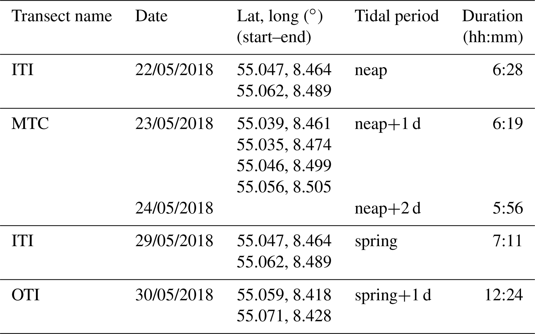
Table 1The summary of the five cruises on board RV Mya II profiling three main transects: the inner tidal inlet (ITI), the main tidal channels (MTC) and the outer tidal inlet (OTI).
3.1 In situ currents and wind data
The observed velocities represented the base for validation of the model and testing of the different tidal open-boundary conditions. The data set is composed of observed profiles of the water currents gathered on five cruises of the RV Mya II (de Luca Lopes de Amorim et al., 2018). The transects cross Lister Deep perpendicularly in two positions: for the outer part, at the narrowest and bathymetrically simplest part of the inlet and for the inner part, because the entire water volume has to pass through this transect, and at the entrance areas to the three main tidal channels (Fig. 1). The cruises were conducted between 22 and 30 May 2018; observations were carried out for half and whole tidal cycles (Table 1). The data were collected using a Teledyne RDI WorkHorse 600 kHz ADCP (Teledyne RD Instruments, San Diego, USA) mounted in the moon pool of the RV Mya II (of the Alfred Wegener Institute) with an offset of 1.3 m related to the water surface. In addition, a differential GPS with a motion sensor worked together with the ADCP to refine and correct the velocity measurements regarding the heading, pitch and roll movements of the ship. Here we would like to stress that the surveys were conducted during different tidal periods (Table 1), which is crucial for high-quality verification.
Wind data were automatically measured by an anemometer mounted on the RV MYA II (summary of the wind conditions can be found in Appendix A, Table A1); the data were obtained from the DAVIS SHIP database for the time of the cruises. The main wind direction during the cruises was around 90∘ (east); the most frequent intensities were in the range of 5 to 10 m s−1. On 24 May the wind was blowing strongly from the east for nearly the whole cruise. Exceptions concerning wind direction were for the cruise on 23 May, when winds were from the NNW (330∘), and the cruise on 29 May, when the most frequent intensity ranged between 10 and 15 m s−1.
3.2 Tide gauge (TG) data
The tide gauge data for the area are represented by three stations: ListTG (55.017∘ N, 8.441∘ E), VidåTG (54.967∘ N, 8.667∘ E) and HavnebyTG (55.087∘ N, 8.565∘ E) (Fig. 1). All data were downloaded from the EMODnet database (the European Marine Observation and Data Network; EMODnet physics database, 2019), which is funded by the European Commission's Directorate General for Maritime Affairs and Fisheries (DG MARE) and provided by the Waterways and Shipping Office in Tönning, the Danish Meteorological Institute and the Danish Coastal Authority. For the spectral analysis, we used data with a 10 min resolution covering the time period from the middle of 2014 through to the end of 2017. The times of the observations are in the UTC (+0) time zone.
4.1 Model validation
Model validation was organized into the following two steps: (1) selection of the best open-boundary conditions using ADCP data and (2) validation of the best open boundary solution against existing tide gauge data, in particular using ListTG, VidåTG and HavnebyTG data. For step (1), the measurements were done during different tidal periods (spring, neap, ebb and flood) in the area of Lister Deep and the main inlets (Fig. 1), which are characterized by the largest depths (up to 35 m) in the domain and by the highest as well as by complex tidally induced velocities. We performed the frequency analysis using the MATLAB package T-TIDE (Pawlowicz et al., 2002) and identified the errors in amplitude and phase for the main tidal constituents (with maximum amplitudes), including higher harmonics.
Table 2The intercomparison of the observed and simulated velocities based on different open-boundary conditions in the area of Lister Deep. The table presents root mean square deviation (RMSD, m s−1) and correlation coefficients (C.C.) for u and v velocity components. The results are given for the simulations performed on the curvilinear grid.

Table 2 represents the root mean square deviation (RMSD) and correlation coefficients of the observed velocities (ADCP data) and the modelled velocities obtained for each open boundary solution. The comparison is based on depth-averaged velocities since the measurements were performed in the deep part of the domain and our task here was to check the performance of the different tidal forcing. In Table 2, results for all the open boundary solutions we used are shown only for the first grid since the difference between the results on different grids is < 0.01 for correlation coefficients and < 0.01 m for the RMSD. However, we would like to note that the unstructured grid provides slightly better results despite its somewhat coarser resolution (the unstructured grid has a larger number of cells, mainly due to detailed representation of the wetting/drying zone). Based on additional experiments (Kuznetsov et al., 2019), we think the reason is that the unstructured grid reflects the bathymetric gradients.
We used different bottom-friction coefficients (Cd) for the different tidal solutions. However, for each run, Cd was spatially uniform as soon as the seabed habitat map is not available yet for the considered area. At the beginning, we took the Cd coefficient as equal to 0.0025 for all simulations. The NEMO solution got much worse results in this case than presented in Table 2 in terms of the RMSD and correlation coefficient (RMSD is larger on average by 15 %, correlation coefficient is less on average by 5 % and 6 % for u and v components, respectively). Further analysis showed that the predicted velocities for the NEMO open boundary solution are too large during some tidal phases. We therefore decided to vary the Cd in a range from 0.002 to 0.004, taking into account the largely sandy bed in the domain, to reach the best agreement with observations (e.g. Werner et al., 2003). Finally, for the TPXO solutions, we used a Cd equal to 0.0025; for the NEMO solution, we used a Cd equal to 0.0035. Note that smaller or larger coefficients did not improve results in terms of RMSD and the correlation coefficient.
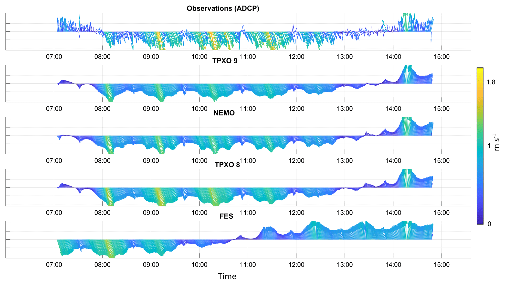
Figure 2The observed and modelled depth-averaged velocities on 29 May 2018. The coloured arrows indicate the current magnitude (m s−1); arrow directions indicate the current direction.
Table 2 shows that the TPXO 9 solution fits the ADCP data best, second best are the TPXO 8.1 and NEMO solutions, and the FES 2014 solution follows. For all solutions except FES, the correlation coefficients are higher during spring tides as well as in the deepest part of the domain; this is true in particular for the measurements performed on 29 and 30 May and despite the quite strong winds often ranging from 10 to 15 m s−1 (Table 1, Fig. 1). On 23 and 24 May, the measurements were performed on nearly the same side, but the 24 May correlation coefficient for the v component is relatively small. This can probably be explained by the permanent wind from the east. We can conclude that tides in that zone explain, on average, more than 80 % (or 90 % or more in the case of a spring tide) of the dynamics in the case of absent storm (more than 20 m s−1) and blowing continuously in one direction winds. Likewise, we conclude that it would be impossible to judge open-boundary-condition quality using information from only one cruise. Figure 2 represents observed and modelled depth-averaged velocities on 29 May (a spring tide). Figure 2 clearly illustrates how the different solutions can align closely at one moment and then begin to deviate greatly at another. Furthermore, the largest velocity errors for all solutions occur when tidal velocities are small as well as during the tidal state change (e.g., in Fig. 2, the time from 07:00 to 08:00 UTC or from 13:00 to 14:00 UTC). This is quite logical, because other effects such as baroclinicity, wind impact and their non-linear interactions then become more pronounced. However, TPXO 9 shows the best agreement with observations during slack tide and provides the smallest RMSD among suggested solutions for all observation days (Fig. 2).
Despite the quite good results of TPXO 8.1 (Table 2), the unstructured grid yields a number of vortex structures near the open boundary that cannot be removed by the sponge layer, which dumps advection and diffusion near the open boundary. It is known that grids that employ an arbitrary normal at the open boundary are subject to the quality of the open boundary signal (Danilov and Androsov, 2015). For TPXO 8.1, the behaviour of the phase is not realistic near the solid boundary: the phase goes through zero simultaneously near the western and eastern solid boundaries.
Table 3Simulated and observed amplitudes (cm) and phases (∘) of the major tidal constituents at different locations.
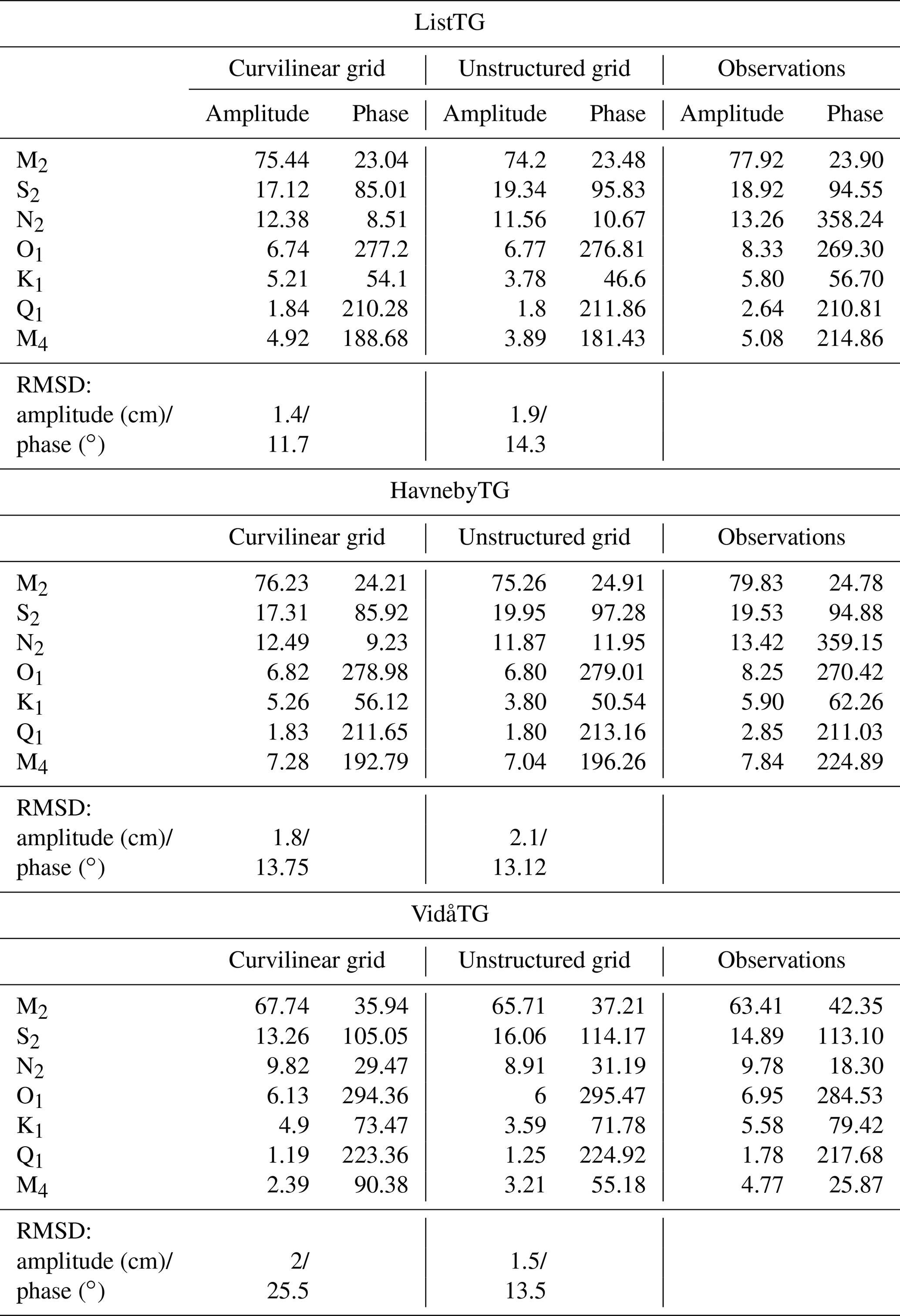
Once we determined the best open-boundary conditions solution – TPXO 9, based on ADCP data – we moved on to the second verification stage. For this, we switched to a 3-D simulation with 10 vertical layers, which are crowding near the sea bed. The optimal roughness height was 0.001 m; this value agreed with the one estimated from observations in a similar region (Werner et al., 2003) and, in terms of the mean, with a Cd equal to 0.0025 for the 2-D scenario. Table 3 presents the results of the frequency analysis of the observational data from the List, Havneby and Vidå TGs as well as from the model using TPXO 9 open-boundary conditions (Taylor diagrams can be found in Appendix B, Fig. B1). Here we present results from both of the grids under consideration. The observed phase values are quite often situated between the values given by the solution on the different grids. This is because we used grid nodes that are nearest to the observational point to perform the analysis, and we did not interpolate the values to the particular coordinates. Either solution (per grid) performed well but each slightly underestimated the amplitudes for major diurnal and semidiurnal constituents (except for the M2 amplitude at the VidåTG). Note that the M2 tidal wave and its subharmonics are shown to vary in amplitude and phase on seasonal, annual and secular timescales (Müller, 2012, 2014; Woodworth et al., 2007; Gräwe et al., 2014). The annual variations in the M2 amplitude are between 6 % and 11 % of the annual mean amplitude for the shallow water stations; the phase could vary by 2 to 6∘ persistently over the last century (Gräwe et al., 2014). The summer amplitudes seem to be larger than the winter amplitudes; this can be explained by changes in thermal stratification (Müller, 2012, 2014; Gräwe et al., 2014). Our simulations obtain “winter” amplitudes, while the observational data provide a mean annual amplitude. The M4 constituent also has a noticeable phase error of at all stations. But, due to large bathymetric uncertainties in the area of the stations, such an inaccuracy is hard to correct (here, the resolution of the bathymetry we used is 50 m). Note that at the Vidå TG, the unstructured grid shows significantly better agreement than the curvilinear grid. This is not surprising since the unstructured grid has much better resolution there.
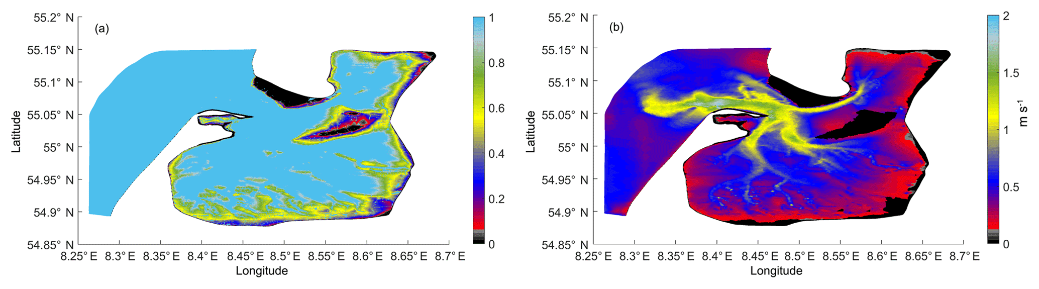
Figure 3(a) The probability of wetting based on simulations of the two full tidal cycles using the unstructured grid. (b) The peak tidal velocities at the current position using the unstructured grid.
4.2 Wetting/drying, maximum tidally induced velocities and tidal prism
Figure 3a shows the probability, in the unstructured grid case, of each node being wet with tidal forcing alone. This figure is based on simulation results for two lunar (synodic) months (29.5 d ×2) after the model reaches a periodic regime. The unstructured grid more accurately represents the wetting/drying zone; it can be traced in smoother forms and in smaller-scale detail than in the curvilinear grid (not shown).
An extensive intertidal subarea situated in the western and southern parts of the considered domain as well as in the Königshafen embayment can be seen, and the Jordsand creates a secondary bight with the Rømø Deep main channel (Figs. 1, 3a).
Figure 3b shows the maximum velocities at each grid point within a lunar (synodic) month. Thus, Fig. 3b shows the highest possible tidally induced velocities in the domain. Figure 3b exhibits, as expected, a correlation with the depth (Fig. 1) but there are many peculiarities which emphasize the large role of non-linear processes in the domain. The maximum velocities can be found at the opening of Lister Deep and near the edge of Sylt during spring ebb and are ∼1.98 m s−1. The tidal prism for the bight varies from 3.3×10⁸ to 6.5×10⁸ m3, with a mean value of 4.8×10⁸ m3; the tidal prism for the whole area varies from 5×10⁸ to 10×108 m3, with a mean value of 7.5×10⁸ m3.
4.3 Energy balance
The analysis of the energy budget and energy flux distribution provides an important insight into the evolution of energy in the modelled region. The energy balance for the vertically averaged equations for the barotropic case has the following form (e.g. Androsov et al., 2002):
where is the total energy per unit area, is the vertically integrated fluid velocity, , ζ is the sea surface elevation, h is the water depth, is the full water depth, ρ is the averaged water density, Cd is the bottom drag coefficient, K is the horizontal eddy viscosity coefficient, g is the acceleration due to gravity and is the nabla operator. Note that we did not introduce horizontal viscosity into our equations; therefore, K equals 0 in our simulations and thus this part of the balance will be omitted. After integration of Eq. (1) over the region Ω with boundary , where ∂Ω1 is the solid part of the boundary and ∂Ω2 is the open boundary, taking into account the Gauss formula for divergence and the condition of zero velocities at ∂Ω1, we obtained the following mean energy balance equation for our depth-averaged solution:
where n is the outward normal to ∂Ω2.
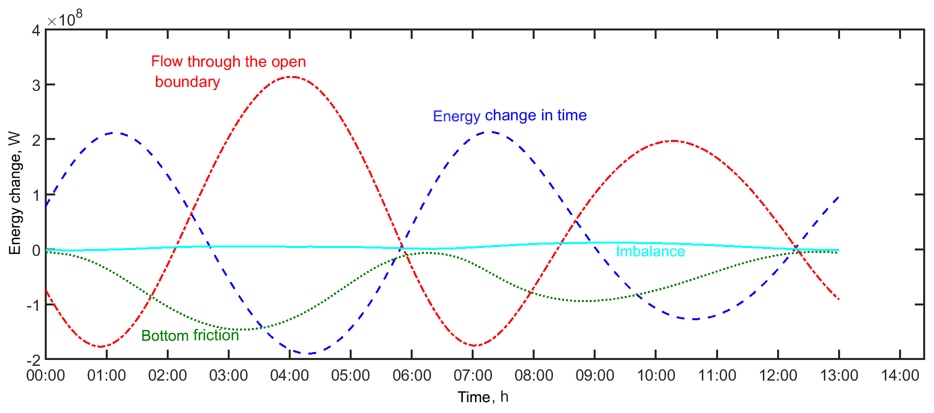
Figure 4The energy budget for the depth-averaged solution with open-boundary conditions from the TPXO 9 database for summary tide, in watts (W): in blue (dashed line) is the energy change in time, in red (dash-dotted line) is the flow through the open boundaries, in green (dotted line) is the bottom friction and in cyan (solid line) is the imbalance.
The first term on the right-hand side of Eq. (2) is the total flux of energy across the open boundary, and the second term is the rate of energy dissipation due to the bottom friction. Figure 4 shows the energy balance for the whole area based on the unstructured grid for the summary tide for one M2 period (the energy balances for the whole area at both grids are visually identical). Once we have different diurnal and semidiurnal constituents in the system, the energy balance every M2 period will not be the same. However, Fig. 4 demonstrates the overall picture. The total energy in the area varies between 7×10¹¹ to 3.5×10¹² J on both grids (in the case of TPXO 8.1 conditions, the total energy in the case of the unstructured grid had different variation limits). For comparison, the full tidal energy in the modelled area is almost equivalent to the full energy of the barotropic tidal dynamics in the Strait of Messina (Androsov et al., 2002), and it is 1 order of magnitude less than in Bab-el-Mandeb Strait (Voltzinger and Androsov, 2008). The potential energy is 1 order of magnitude larger than the kinetic energy. The shares of the total energy based on the open boundary information are distributed in the following way: M2 brings 58 %, S2 brings 13.5 %, N2 brings 10 %, K2 brings 3.5 %, K1 brings 4 %, O1 brings 5.5 %, P1 brings 1 %, and the Q1 and M4 components bring 1.5 % and 3 %, respectively. The fluxes through the open boundary can remove up to 1.5×10⁸ J s−1. Bottom friction takes up a significant amount of energy, on average 6.4×10⁷ J s−1, due to the shallowness of the bight (Fig. 4). The imbalance is 2 orders of magnitude smaller than the energy change. The unstructured grid is a bit more dissipative; its imbalance is 10 % larger than that on the curvilinear grid. This is for several reasons: the unstructured grid in particular contains triangles, arbitrary quads and, in some places, large gradients in grid cell size, which cause additional noise (Danilov and Androsov, 2015). We would like to point out that it is hard to estimate the numerical dissipation rate precisely. The current imbalance consists not only of numerical dissipation but also of uncertainties in the energy balance calculation once we no longer accounted for the role of the explicit time-difference scheme with an Adams–Bashforth extrapolation and the effects of velocity filtration. Our additional runs showed that the impact of these procedures has the same magnitude as a calculated imbalance. We think that, on the curvilinear grid, the real imbalance due to numerical viscosity is close to zero, at least 1 order of magnitude smaller than the presented one.
The maximum change in system energy and maximum fluxes through the open boundaries take place during ebb tide; the ebb phase duration is, on average, 0.85 of the flood phase. These general conclusions mask very patchy dynamics in the area, which are considered in detail in the next sections.
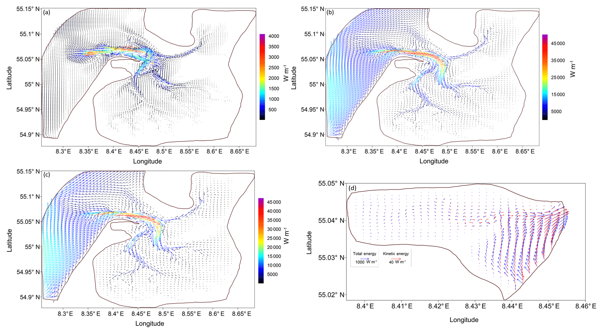
Figure 5The flux of tidal energy (summary tide): (a) kinetic; (b) potential; (c) total (EλEθ); and (d) the total (blue arrows) and kinetic (red arrows) energy fluxes for the Königshafen subarea. The potential energy flux behaviour is visually identical to the total energy fluxes behaviour.
Figure 5 demonstrates the energy fluxes in the area. The tidal energy flux, represented by the sum of the potential and kinetic energy fluxes, is estimated using the following definition (Crawford, 1984; Kowalik and Proshutinsky, 1993):
where Eλ and Eθ are the zonal and meridional components of the tidal energy flux vector, and T is the full tidal period (synodical month – 29.5 d). Figure 5a, b and c show that the potential energy fluxes in the area are 1 order of magnitude larger than the kinetic energy fluxes. Therefore, total energy fluxes are largely defined by potential energy fluxes (Fig. 5b, c). It can be noted that the directions of the potential and kinetic energy fluxes can deviate from each other and be opposite (Fig. 5a, b); this can be explained easily by the fact that the kinetic energy fluxes largely reflect dissipation of the energy, and the potential energy fluxes largely reflect energy distribution pathways in the domain. So, in Fig. 5b and c, it can be seen that the dynamics in the external part of the domain are determined by the Kelvin wave coming from the south-west. Obviously, the bulk of the energy comes into the internal part of the domain through Lister Deep. The energy leaves the whole modelling domain mostly through the north-eastern part of the open boundary. Figure 5d demonstrates that the bulk of the energy comes to Königshafen from the south and circulates there through the system of gyres (the curl part of the energy fluxes is larger than the divergence part). Figure 5d also indicates that the energy fluxes along the coastline in this subarea are opposite in direction to those within the main channel.
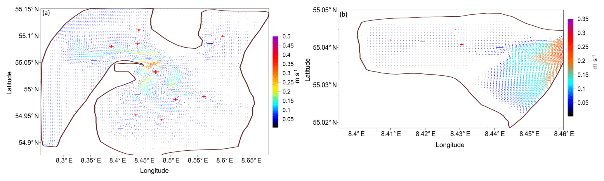
Figure 6Residual circulation of the summary tide for (a) the whole area considered and (b) the Königshafen embayment. The “+'` and “−” symbols illustrate the clockwise and anticlockwise rotation, respectively, of the major gyres present in the system. The residual circulation is demonstrated on the unstructured grid.
4.4 Residual circulation
The residual circulation in the area is characterized by the large number of vortex structures with different rotation directions in the area of Lister Deep and the main channels (Figs. 1, 6a). Note that the residual circulation in the external part of the domain is defined by kinetic energy fluxes, because here the role of non-linearity in the continuity equation is minor (the water depth compared to the tidal amplitude is relatively large). These vortexes organize a complex residual circulation pattern; the strongest circulation (up to 0.45 m s−1) can be found in the area of Lister Deep, where different incoming and outgoing flows meet, and in the other areas of large bathymetric gradients. Note, that the two largest vortex structures in terms of the residual velocities magnitude, which show opposite rotational, were also resolved by Burchard et al. (2008) and Ruiz-Villarreal et al. (2005) based only on the M2 signal. Near Königshafen we can also follow the gyre system in the opposite direction, which alternates (Fig. 6b). Note that, here, the energy fluxes and residual circulation patterns have much in common. The bulk of the energy fluxes come from the south, and tides lose energy on the way, causing residual circulation shaped by the bathymetric features. For this subarea, the residual velocities are less than 0.05 m s−1. The residual circulation in the external part of the domain shows that the bulk of water masses penetrate to the internal part of the domain from the western boundary and the south, moving along the coast. Water masses mainly leave the domain through the central part of the open boundary. Such a complex residual circulation (Fig. 6) signals potential difficulties in calculating sediment budget.
4.5 Tidal ellipses
The resulting movement in the SRB represents a superposition of the tidal waves reflected off the region's solid boundaries. As a result of this interference, a standing wave occurs, containing only one component of the velocity for the main tidal harmonics, which is to say currents are close to reverse. The Coriolis effect does not lead to significant cross-currents. Figure 7a and b show the ellipses of the wave M2 and S2 tidal currents, respectively; the character of the currents of either wave component is practically indistinguishable in the SRB except for the amplitude of the M2 velocity, which turned out to be almost 4 times larger than the amplitude of the S2 velocity. The direction of rotation of the velocity vector is determined by the sign of the ellipticity. A negative ellipticity value means that the tidal current vector rotates anticyclonically. The anticyclonic rotation of the depth-averaged velocities near Sylt-Rømø is inherent only in zones of a significant bathymetric gradient where maximum tidal currents are observed. This kind of rotation has to overcome the Coriolis effect, which spins in the opposite direction. At the same time, on the boundary with the North Sea (the open boundary of the modelled region), the currents have a constant cyclonic rotation, which corresponds to the cyclonic movement of the Kelvin wave along the coast in the Northern Hemisphere.
The ellipses induced by the M4 wave are shown in Fig. 7c. This picture differs from the main tidal harmonic frequencies in the presence of mixed flow zones. In deep-water channels, the currents are close to reverse during the tidal cycle, and on the shape of bathymetry the transverse velocity component appears. The amplitude of the velocity of the M4 wave reaches 25 cm s−1 in most bottlenecks of the modelled region and near Königshafen. Near the open boundary, the currents have a pronounced anticyclonic character, i.e. non-linear flows overcome the Coriolis effect, spinning the flow in the opposite direction. In some areas around the shallow zones, the major axis of the M4 ellipsis is at a significant angle to the major axis of the M2 ellipsis. This can lead to secondary circulation in a rotating system.

Figure 7Axes of the (a) M2, (b) S2 and (c) M4 tidal current ellipses and zones of the minor-to-major axis ratios. Yellow zones denote the domain of anticyclonic rotation of the current vector.
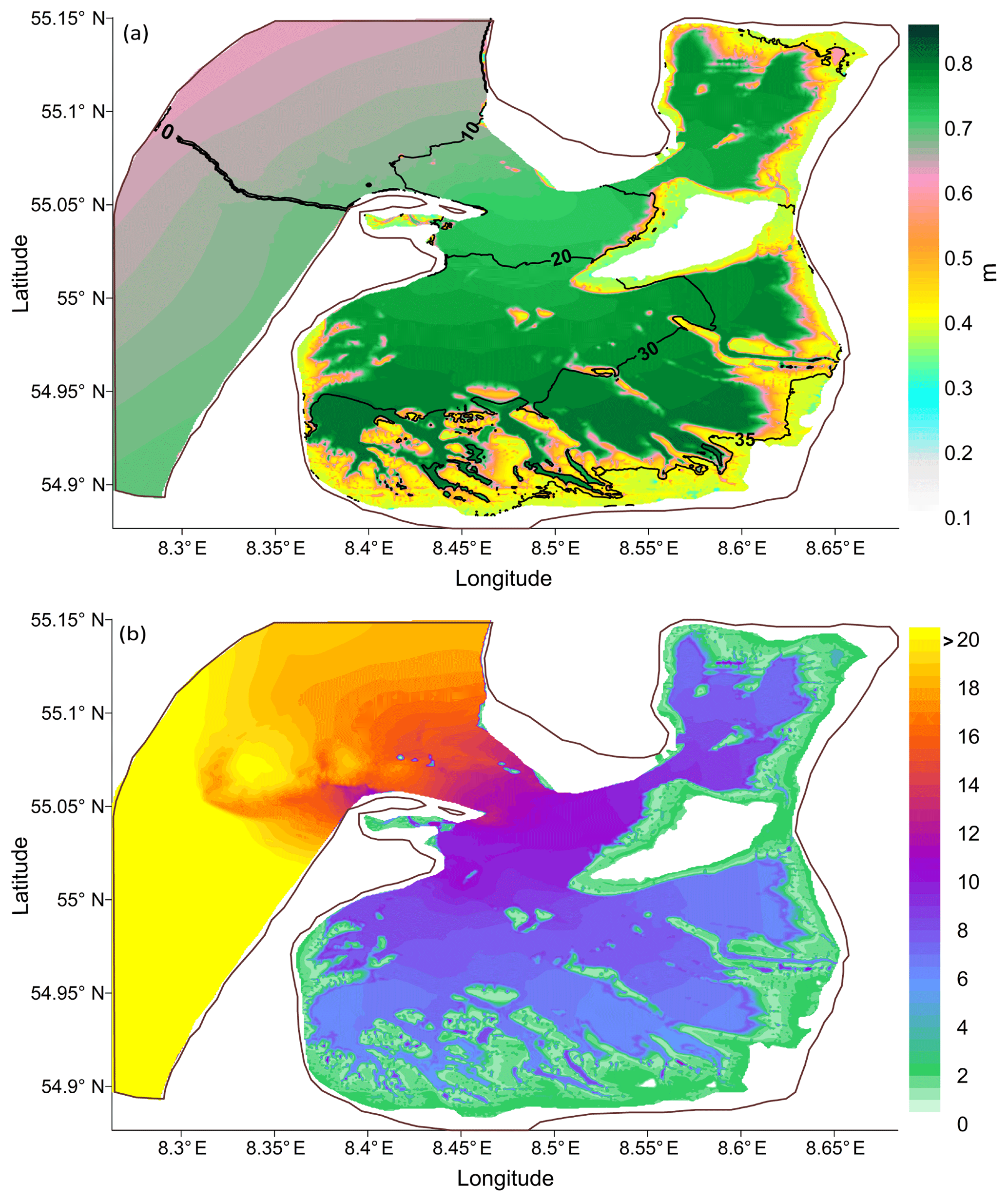
Figure 8(a) The relative weight of the linearity: the ratio of M2 wave amplitude to the sum of the major non-linear constituents. (b) Tidal map for the M2 wave: phases (∘) are demonstrated via contour lines, amplitudes (m) are demonstrated via the colour bar. The maps were created based on elevation data analysis. The white colour indicates zones where topography features are above 0 m sea level.
4.6 Non-linearity structure and tidal asymmetry
The major higher harmonics in the area are M4 with 36.6 % of total energy attributed to the non-linear harmonics in the whole considered domain, M6 with 12.43 %, MS4 with 12.27 %, MN4 with 10.95 %, M8 with 6.43 %, 2MS6 with 5.6 %, 2MN6 with 5.23 %, MO3 with 4.73 %, SN4 with 4.08 %, S4 with 0.92 %, and 2SM6 with 0.75 %. These numbers were calculated based on a weighted sum of the harmonic amplitudes. Figure 8 shows the relative role of these higher harmonics compared to the M2 signal and the tidal map for the M2 wave. In particular, Fig. 8a demonstrates the ratio of the M2 amplitude to the sum of amplitudes of the listed higher harmonics. The role of non-linear harmonics becomes significant in the interior zone of the domain, increasing with greater distance from the bottleneck and near the wetting/drying zone (Figs. 3a, 8). To quantify the role of the higher harmonics, Fig. 8b also demonstrates the tidal map for the M2 wave. The M2 wave amplitude is greatest in the southern part of the internal area.
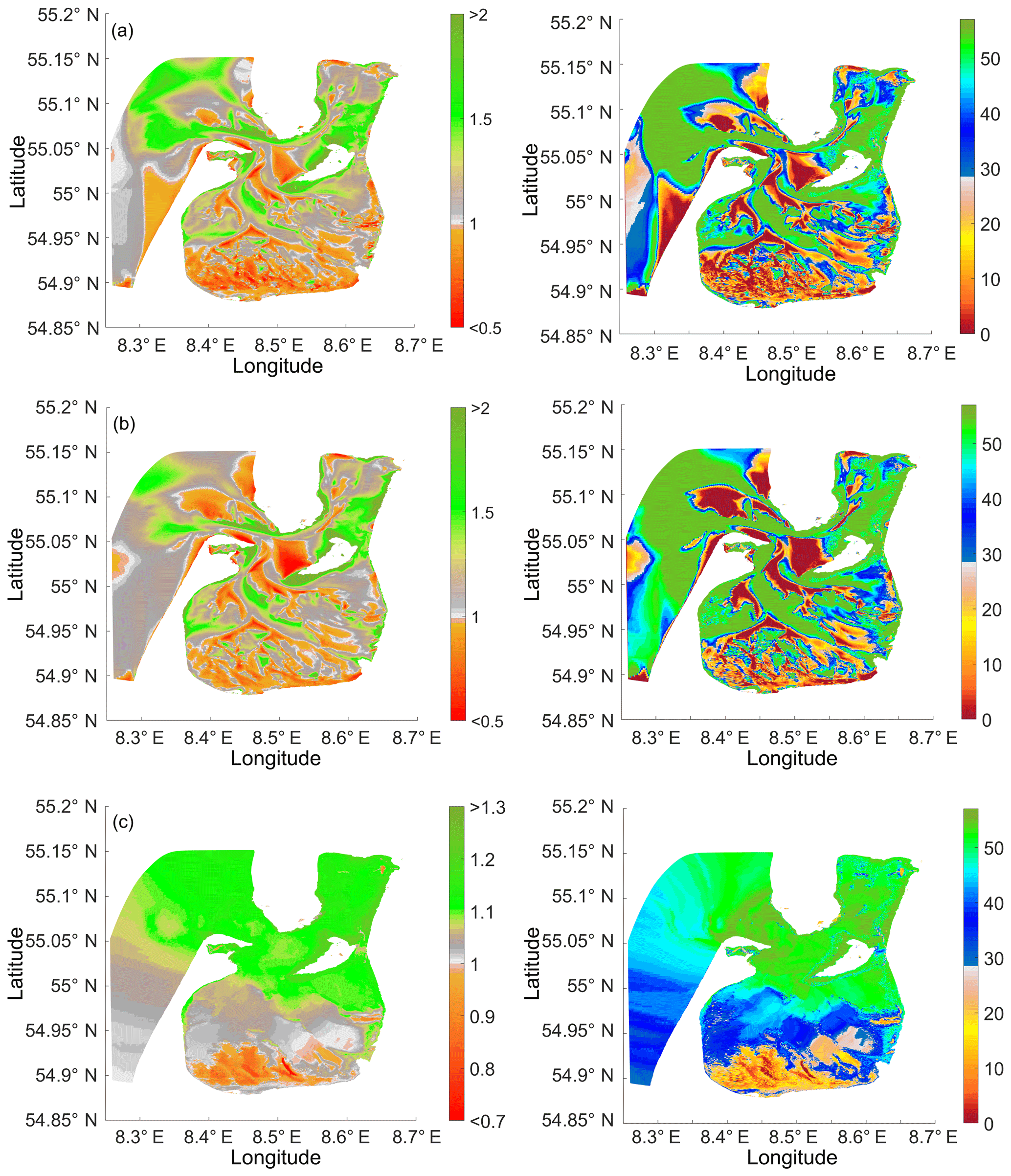
Figure 9The ebb-flood dominance asymmetry maps. Left panels: ratio of (a) maximum velocities during ebb and flood, (b) mean velocities during ebb and flood, and (c) durations of flood and ebb. Right panels: frequency of event within a lunar (synodic) month (amount of the tidal cycles) (a) maximum velocities during ebb are higher than during flood, (b) mean velocities during ebb are higher than during flood, and (c) flood is longer than ebb. Numbers 1–4 indicate different zones under consideration. The A, B demonstrates an example of the subareas in which the strong flood dominance in terms of velocity does not mean shorter flood. Subareas which do not take part in at least one flood–ebb cycle are removed.
The domain configuration and the foregoing results of the tidal energy transformation and evolution are signals of a pronounced tidal asymmetry in the tidal water level and in the current velocity behaviour in the area. There are several reasons for the tidal asymmetry – in particular, the presence of the non-linear advection and bottom friction terms together with complex topography, resulting in a non-trivial wave interaction in the system (e.g. Friedrichs and Aubrey, 1988). The key geometric features directly impacting tidal distortion are the bathymetry relative to the tidal amplitude, the bottleneck width and its variation during the tidal cycle, as well as the area occupied by the intertidal zone and its distance to the main tidal inlets. For data about tidal asymmetry to inform sediment dynamics analysis, we concentrate on the ebb and flood durations as well as the mean and maximum velocity relations. Ebb is defined as a period when the water level at the current location is decreasing, and flood is defined as the period when it is increasing. Figure 9a (left panel) represents the ratio between the maximum velocities during spring ebb and flood. Figure 9b (left panel) represents the ratio of mean velocities during ebb and flood periods. Figure 9c (left panel) represents the ratio of mean ebb and flood durations. The analysis reflects near-bottom velocities; however, the pattern of ratios is nearly the same for the depth-averaged solution. We note generally that the near-bottom solution provides a more pronounced ebb or flood dominance. The features represented in Fig. 9 (left panel) show the mean pattern for a lunar (synodic) month (29.5 d). In such a domain, we can expect that the flood–ebb dominance feature is not constant but can change within a lunar (synodic) month. For some ebb–flood cycles, the picture presented in Fig. 9 (left panel) can be significantly different. Therefore, we have decided to calculate how often flood or ebb dominance takes place within a lunar (synodic) month in terms of velocities and duration.
Figure 9 (right panel) comprises 57 floods and ebbs. (We considered 28.5 d, but the first and last flood and ebb of the lunar (synodic) month – 29.5ḋ – were removed to make sure that we were considering the beginning of the flood and ebb.) Then we calculated how often the mean and maximum velocities of the ebb are larger during the following flood (Fig. 9a, b right panels). We also calculated how often the ebb duration was smaller than that of the following flood (Fig. 9c, right panel). In other words, Fig. 9a (right panel) shows for example the frequency of the maximum velocity during ebb being larger than that of the following flood; a value of 57 means that across all 57 cycles, maximum velocities during ebb are larger than during flood. We should note that flood or ebb dominance is caused not only by non-linear effects but also due to the diurnal inequality of tide. From all these pictures, we have removed subareas which did not take part at least one flood–ebb cycle.
Figure 9 was generated from simulations on the curvilinear grid. But an important result is that the difference between the ratios (asymmetry indicators) on either grid touches only a few details, but not a general pattern. The maximum disagreement occurred during comparison of the ratios of velocities, going up to 0.2 for ratios of mean and maximum velocities. However, we would like to stress that the position of the ebb and flood dominance areas are the same with only a small difference at the edge of the zones.
The patterns presented in the left and right panels show some common features, and this is to be expected. For example, if the ebb velocities are larger than the flood velocities in nearly every ebb–flood cycle, then the averaged value of the velocity ratios will be large, and the corresponding figure in the right panel will show a high frequency of the ebb-dominance event. Figure 9 (right panel) shows that there are a lot of zones that may behave differently during different periods of a lunar (synodic) month. (The frequency is between 0 and 57.) Note also that Fig. 9a and b represent largely different patterns than Fig. 9c. For, example, if the mean and maximum velocities in the internal part of the domain are larger during flood, it does not mean that the flood will be shorter. There can be no mass conservation for the ebb–flood cycle for the particular area subunit. Note that the ebb in the whole domain under consideration is typically shorter than the flood, except in the south-western part of the internal area (Fig. 9c, left panel).
Figure 9 demonstrates that it is not correct to regard ebb or flood dominance based only on velocity characteristics or typical flood or ebb durations when these characteristics can yield opposite answers. Additionally, these characteristics are not necessarily the same within one lunar (synodic) month (29.5 d).
To explain the complexity of the presented pattern, we have split the domain under consideration into four parts designated as zones 1 through 4 (Fig. 9a, left panel).
4.6.1 Zone 1
Zone 1 represents an area where we observe a progressive Kelvin wave (Figs. 5, 9). The flood-dominated (orange-coloured) zone, in terms of maximum velocities (Fig. 9a, left panel), matches the area where we have a comparatively small residual circulation (Fig. 6). Gravity waves traverse the shallow zone non-dispersively at a speed defined by (g is acceleration due to gravity, H is the full depth), so we suggest that the crest of the tide overtakes the trough here (e.g. Dronkers, 1986; Hayes, 1980; Saloman and Allen, 1983). This is confirmed by Fig. 9a (right panel), which shows that maximum velocities in this zone are nearly always larger during flood. Figure 9b (left panel) shows that mean velocities in this subzone are nearly equal to each other in terms of the mean, with slight ebb dominance. However, also some tidal cycles exhibit larger mean flood velocities than mean ebb velocities (Fig. 9b, right panel).
4.6.2 Zone 2
In zone 2, we have an extensive intertidal zone and maximum amplitudes of the semidiurnal tides compared to other zones; also, this zone lies far from the Lister Deep area. In this zone, the role of higher harmonics is greatest (Fig. 8), revealing the major role of non-linear friction effects and non-linearity in changes of the water-layer thickness: here, the ratio of tidal amplitude to depth is greatest (increasing from Lister Deep toward the southern part of the zone). This also can be seen in Fig. 7, which shows M4 locked in a velocity phase of −90 to 90∘ relative to M2. As a result, water level changes propagate more slowly during ebb (Dronkers, 1986), and the time delay between low water at the inlet to Lister Deep versus in the considered area is greater than that for high water. In every regard, the farther away from Lister Deep, the more pronounced the flood dominance becomes. This means that ebb duration increases, and velocities are larger during flood.
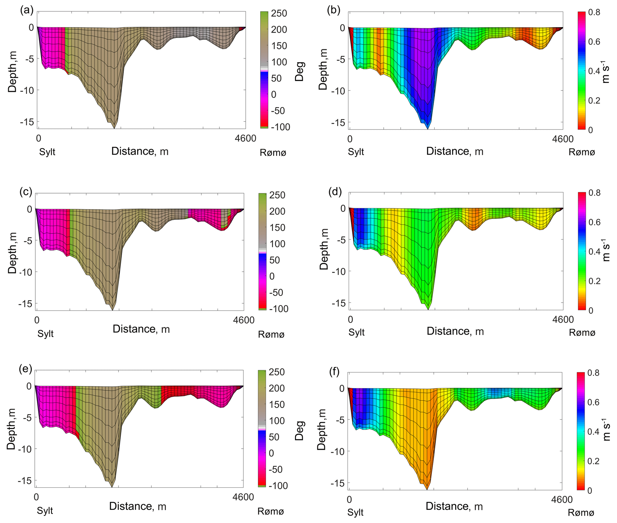
Figure 10Snapshots of direction relative to the y axes (counted positively anticlockwise) (∘) and magnitude (m s−1) of velocities within the cross-section which connects Sylt (left shore) and Rømø (right shore); the angle between y axes and the cross-section is . In the left panel, the grey-green colour indicates water outflow; blue-red colour indicates water inflow. The snapshots capture the transition phase from ebb to flood with a 20 min interval from one picture to another (top to bottom). The top panel is a snapshot of a moment when the external part of the domain is already at first-stage flood and the internal part of the domain is still at last-stage ebb.
4.6.3 Zone 3
In zone 3 we have very patchy dynamics in terms of velocities during flood and ebb (there are a lot of subzones characterized by the flood dominance and ebb dominance); however, it is typical for the whole area that ebb is shorter than flood (flood duration is between 1.1 and 1.3 of ebb duration). Lister Deep can be characterized generally by higher mean and maximum velocities during ebb, but some side channels can be characterized by higher velocities during flood. As the tide turns at low water, strong currents are still flowing seaward out of the main ebb channel. As the water level rises, the flood currents seek the path of least resistance around the margin of the delta. This creates horizontal segregation of flood and ebb currents in the tidal channels for a time. This is apparent in Fig. 10, depicting the transitional moment from ebb to flood.
In this zone, we emphasize subareas A and B as prime examples of the subdomains where mean current ratio and maximum current ratio (Fig. 9a, b) are not synchronized with the durations ratio (Fig. 9c). For example, Fig. 9a and b demonstrate that the velocities at B are larger during flood in terms of the mean and maximum; but flood duration is longer than ebb. This signals that the water parcels are travelling different pathways during flood and ebb.
4.6.4 Zone 4
Zone 4 represents a small semi-enclosed bight with a flood-dominated main channel and an ebb-dominated area around, as well as in the inner part of the bight in terms of velocity. However, we would like to stress that flood dominance, though typical, is not a constant feature. For several cycles within a lunar (synodic) month (29.5 d), the mean and maximum velocities will be larger during ebb. For the whole zone, ebb is shorter than flood for almost a lunar (synodic) month. The reason the pattern is opposite to that of zone 3 lies in the small volume of intertidal storage and large variation in the “main channel” width. In this zone, frictional drag is insignificantly greater at low water than at high water. Also, the role of M4 tide compared to M2 tide is greatest there (not shown); the role of the sum of all non-linear harmonics is smaller than in zone 2 (Fig. 8). For this zone, ebb and flood generally start on the sides of the main channel, Rømø Deep, in marginal ebb-dominated channels.
5.1 Bedform peculiarities
The most interesting question for future study is how the given asymmetry and residual circulation pattern line up with the bedform peculiarities. Therefore, the next step will be an intercomparison between measurements in the frame of the planned multibeam echosounder surveys and results of the current paper. The prediction of the bedform peculiarities in the area requires a coupled sediment module as well as wind and wave forcing. However, as soon as we have shown (Table 2, Fig. 2) that tides can explain a large part (more than 80 %) of the current velocities in the area of Lister Deep, some prognoses can be made at the current stage. The results suggest the presence of subaqueous dunes with stable characteristics in areas where mean and maximum current velocities are permanently higher or lower during ebb and flood than during flood and ebb. With this definition (see Fig. 9), our results agree with those presented in Boldreel et al. (2010) and Mielck et al. (2012). In those studies, conducted in the working area of Lister Deep and adjacent to Königshafen, dunes of various sizes, escarpments and other erosional features were analysed based on hydro-acoustic data (seismic profiles, side-scan sonar and the RoxAnn seafloor classification system) to determine dune characteristics and orientations (and hence flood or ebb dominance) of the particular areas. Boldreel et al. (2010) state that the flood-dominated dunes are larger than ebb-dominated dunes in the area of the bottleneck. Our study reveals that, in this zone, the ebb is generally shorter than the flood (Fig. 9c), which may explain this observation. The map of the residual circulation (Fig. 6) suggests probable directions of subaqueous dune migration where bottom currents are strong enough.
5.2 Grid performance
Each presented grid has advantages and disadvantages. The curvilinear grid offered minimum numerical viscosity but was not very flexible when it came to choosing grid cell size as compared to an unstructured grid (see also, Figs. A1, A2; Danilov and Androsov, 2015; Androsov et al., 2019). This is especially crucial in the zones of large bathymetric gradients and in the wetting/drying zones. The unstructured grid is more dissipative and more sensitive to the quality of the open boundary solutions. The reproduction of the non-linear effects on the grids of different structures represents an additional scientific question, which should be disentangled in the future.
This study is dedicated to tidally induced dynamics in the SRB, with a focus on the non-linear component. The newly obtained high-quality bathymetric data supported the use of high-resolution grids (up to 2 m in the wetting/drying zone) and elaboration of the details of tidal energy transformation in the domain. The FESOM-C model was used as the numerical tool. In preparation, different open-boundary conditions for the summary tide (major diurnal and semidiurnal as well as M4 constituents) were tested for the best fit with observational data. The simulations with open-boundary conditions from TPXO 9 showed very satisfying agreement with available observations. Based on 3-D barotropic runs, the ellipses, energy fluxes, residual circulation and tidal asymmetry maps were constructed and analysed for the whole area for the first time. Four zones with fundamentally different asymmetry structures were indicated during tidal asymmetry analysis. We also showed that it is not correct to talk about ebb or flood dominance based only on one velocity characteristic or typical flood or ebb durations since these indicators can yield an opposite answer. Also asymmetry indicators were not constant everywhere from one ebb–flood cycle to another.
All experiments were performed on two grids with different structures and resolution details. Energy balance fulfilment was shown for both grids. The generated maps generally showed the same pattern on both grids, which allowed us to conclude that further increasing the resolution will not lead to pronounced changes in the results. The obtained results are a necessary and useful benchmark for further studies in the area, including for work on baroclinic and sediment dynamics. It would be fruitful to pursue further research about how the obtained maps reflect bedform peculiarities in the area in order to predict bedform characteristics in the shallow zones, which are hard-to-reach places for the ship surveys.
The observed profiles of the water currents gathered on five cruises of the RV Mya II can be found in the PANGAEA database (https://doi.org/10.1594/PANGAEA.894070; de Luca Lopes de Amorim et al., 2018). The tidal open boundary conditions can be downloaded from TPXO (https://www.tpxo.net/global; TPXO database, 2019; Egbert and Erofeeva, 2002), AVISO (https://www.aviso.altimetry.fr/en/data/products/auxiliary-products/global-tide-fes/description-fes2014.html; AVISO database, 2019; Carrere et al., 2016) and Copernicus Marine databases (http://marine.copernicus.eu/services-portfolio/access-to-products/?option=com_csw&view=details&product_id=NORTHWESTSHELF_ANALYSIS_FORECAST_PHY_004_013; Copernicus Marine Database, 2019; Tonani et al., 2019). The tide gauge data for the area can be downloaded from the EMODnet database (http://www.emodnet-physics.eu/Map/; EMODnet physics database, 2019). The version of FESOM-C v.2 used to carry out simulations reported here can be accessed from ZENODO data portal (https://doi.org/10.5281/zenodo.2085177; Androsov et al., 2018). The grids for the presented setups can be provided by the request.
Table A1Summary of the five cruises on board of RV Mya II, profiling three main transects: inner tidal inlet (ITI), main tidal channels (MTC) and outer tidal inlet (OTI). Main tidal channels (MTC) show the initial, turning and ending points, since it covers three sections in one transect. The wind roses characterize the wind conditions during cruise times, with the legend colours representing the wind velocity (m s−1) and the circles representing the frequency percentage of the direction from where the wind blows.
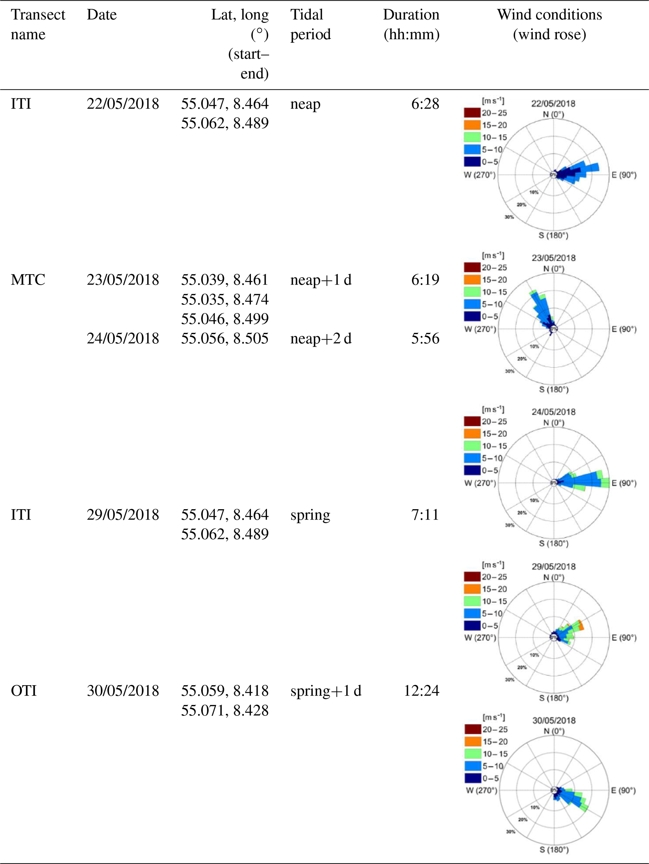

Figure A1Nodal area where the pink colour indicates the position of the open boundary: (a) curvilinear grid and (b) unstructured grid.
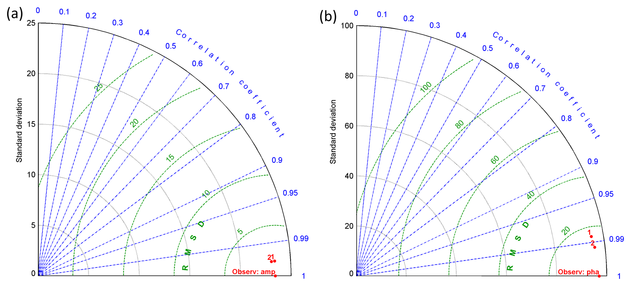
Figure B1Taylor diagrams based on observed and modelled data at three gauging stations, “1” and “2” indicate simulation results on curvilinear and unstructured grids, respectively: (a) for amplitude; (b) for phase.
VF designed the experiments, carried them out, prepared the unstructured grid and new bathymetry product, and suggested asymmetry analysis. AA constructed the curvilinear grid, encouraged VF to investigate some aspects of the non-linear dynamics, wrote the part about tidal ellipses and helped to visualize the results. LS carried out and provided the multi-beam data, participated in the construction of the new bathymetry product, and consulted VF a lot during the verification stage. IK and HCH discussed with VF all experiments and results providing valuable comments and remarks. FA carried out and processed ADCP data, prepared the reference list, and, together with HCH and LS, significantly improved the article readability. HCH provided the information about bedform peculiarities in the area. KHW supervised the research. All authors contributed to the final article, provided critical feedback and helped to shape the research.
The authors declare that they have no conflict of interest.
This article is part of the special issue “Developments in the science and history of tides (OS/ACP/HGSS/NPG/SE inter-journal SI)”. It is not associated with a conference.
Authors are indebted to Hans Burchard for the useful remarks and fruitful discussion and to Natalja Rakowsky and Sven Harig for the technical support. Also we are grateful to the three anonymous reviewers for the valuable comments and suggested improvements to the article.
The article processing charges for this open-access publication were covered by a Research Centre of the Helmholtz Association.
This paper was edited by Mattias Green and reviewed by three anonymous referees.
Androsov, A., Fofonova, V., Kuznetsov, I., Danilov, S., Rakowsky, N., Harig, S. Brix, H., and Wiltshire, K. H.: FESOM-C, https://doi.org/10.5281/zenodo.2085177, 2018.
Androsov, A., Fofonova, V., Kuznetsov, I., Danilov, S., Rakowsky, N., Harig, S., Brix, H., and Wiltshire, K. H.: FESOM-C v.2: coastal dynamics on hybrid unstructured meshes, Geosci. Model Dev., 12, 1009–1028, https://doi.org/10.5194/gmd-12-1009-2019, 2019.
Androsov, A. A., Klevanny, K. A., Salusti, E. S., and Voltzinger, N. E.: Open boundary conditions for horizontal 2-D curvilinear-grid long-wave dynamics of a strait, Adv. Water Resour., 18, 267–276, https://doi.org/10.1016/0309-1708(95)00017-D, 1995.
Androsov, A. A., Kagan, B. A., Romanenkov, D. A., and Voltzinger, N. E.: Numerical modelling of barotropic tidal dynamics in the strait of Messina, Adv. Water Resour., 25, 401–415, https://doi.org/10.1016/S0309-1708(02)00007-6, 2002.
AVISO database: FES2014 product: Carrere, L., Lyard, F., Cancet, M., Guillot, A., Dupuy, S., available at: https://www.aviso.altimetry.fr/en/data/products/auxiliary-products/global-tide-fes/description-fes2014.html, last access: 11 December 2019.
Austen, I.: The surficial sediments of Königshafen – variations over the past 50 years, Helgolander Meeresun., 48, 163–171, https://doi.org/10.1007/BF02367033, 1994.
Becherer, J., Burchard, H., Flöser, G., Mohrholz, V., and Umlauf, L.: Evidence of tidal straining in well-mixed channel flow from microstructure observations, Geophys. Res. Lett., 38, L17611, https://doi.org/10.1029/2011GL049005, 2011.
Bolaños-Sanchez, R., Riethmüller, R., Gayer, G., and Amos C. L.: Sediment transport in a tidal lagoon subject to varying winds evaluated with a coupled current-wave model, J. Coast. Res., 21, e11–e26, https://doi.org/10.2112/03-0048.1, 2005.
Boldreel, L. O., Kuijpers, A., Madsen, E. B., Hass, H. C., Lindhorst, S., Rasmussen, R., Nielsen, M.G, Bartholdy, J., and Pedersen, J. B. T.: Postglacial sedimentary regime around northern Sylt, South-eastern North Sea, based on shallow seismic profiles, B. Geol. Soc. Denmark, 58, 15–27, 2010.
Burchard, H., Flöser, G., Staneva, J. V., Riethmüller, R., and Badewien, T.: Impact of density gradients on net sediment transport into the Wadden Sea, J. Phys. Oceanogr., 38, 566–587, https://doi.org/10.1175/2007JPO3796.1, 2008.
Carrere, L., Lyard, F., Cancet, M., Guillot, A., and Picot, N.: FES 2014, a new tidal model – Validation results and perspectives for improvements, ESA Living Planet Conference, Prague, Czech Republic, 9–13 May, 2016, ESA Living Planet Symposium, 2016.
Crawford, W. R.: Energy flux and generation of diurnal shelf waves along Vancouver Island, J. Phys. Oceanogr., 14, 1600–1607, https://doi.org/10.1175/1520-0485(1984)014<1600:EFAGOD>2.0.CO;2, 1984.
Copernicus Marine Databases: Atlantic – European North West Shelf – Ocean Physics Analysis and Forecast, the data provided by Copernicus Marine Environment Monitoring Service, available at: http://marine.copernicus.eu/services-portfolio/access-to-products/?option=com_csw&view=details&product_id=NORTHWESTSHELF_ANALYSIS_FORECAST_PHY_004_013, last access: 11 December 2019.
Danilov, S. and Androsov, A.: Cell-vertex discretization of shallow water equations on mixed unstructured meshes, Ocean Dynam., 65, 33–47, https://doi.org/10.1007/s10236-014-0790-x, 2015.
Danilov, S., Sidorenko, D., Wang, Q., and Jung, T.: The Finite-volumE Sea ice–Ocean Model (FESOM2), Geosci. Model Dev., 10, 765–789, https://doi.org/10.5194/gmd-10-765-2017, 2017.
de Luca Lopes de Amorim, F., Sander, L., and Hass, H. C.: Raw data of continuous VM-ADCP (vessel-mounted Acoustic Doppler Current Profiler) profiles and DGPS during five cruises on board of MYA II in the Sylt-Rømø Bight. Alfred Wegener Institute – Wadden Sea Station Sylt, PANGAEA, https://doi.org/10.1594/PANGAEA.894070, 2018.
Dronkers, J.: Tidal asymmetry and estuarine morphology, Neth. J. Sea Res., 20, 117–131, https://doi.org/10.1016/0077-7579(86)90036-0, 1986.
Egbert, G. D. and Erofeeva, S. Y.: Efficient inverse modeling of barotropic ocean tides, J. Atmos. Ocean. Tech., 19, 183–204, https://doi.org/10.1175/1520-0426(2002)019<0183:EIMOBO>2.0.CO;2, 2002.
EMODnet physics database: Sea elevation data provided by the Waterways and Shipping Office in Tönning, the Danish Meteorological Institute and the Danish Coastal Authority, available at: http://www.emodnet-physics.eu/Map/, last access: 11 December 2019.
Friedrichs, C. T. and Aubrey, D. G.: Non-linear tidal distortion in shallow well-mixed estuaries: a synthesis, Estuar. Coast. Shelf S., 27, 521–545, https://doi.org/10.1016/0272-7714(88)90082-0, 1988.
Gätje, C. and Reise, K. (Eds.): Ökosystem Wattenmeer: Austausch-, Transport- und Stoffumwandlungsprozesse, Springer, Berlin, Heidelberg, Germany, https://doi.org/10.1007/978-3-642-58751-1, 1998.
Gräwe, U., Burchard, H., Müller, M., and Schuttelaars, H. M.: Seasonal variability in M2 and M4 tidal constituents and its implications for the coastal residual sediment transport, Geophys. Res. Lett., 41, 5563–5570, https://doi.org/10.1002/2014GL060517, 2014.
Gräwe, U., Flöser, G., Gerkema, T., Duran-Matute, M., Badewien, T. H., Schulz, E., and Burchard, H.: A numerical model for the entire Wadden Sea: Skill assessment and analysis of hydrodynamics, J. Geophys. Res.-Oceans, 121, 5231–5251, https://doi.org/10.1002/2016JC011655, 2016.
Gurvan, M., Bourdallé-Badie, R., Bouttier, P-A., Bricaud, C, Bruciaferri, D., Calvert, D., Chanut J., Clementi, E., Coward, A., Delrosso, D., Ethé, C., Flavoni, S., Graham, T., Harle, J., Iovino, D., Lea, D., Lévy, C., Lovato, T., Martin, N., Masson, S., Mocavero, S., Paul, J., Rousset, C., Storkey, D., Storto, A., and Vancoppenolle, M.: NEMO ocean engine (Version v3.6), Notes du Pôle de Modélisation de L'institut Pierre-Simon Laplace (IPSL), Zenodo, https://doi.org/10.5281/zenodo.1472492, 2017.
Hayes, M. O.: General morphology and sediment patterns in tidal inlets, Sediment. Geol., 26, 139–156, https://doi.org/10.1016/0037-0738(80)90009-3, 1980.
Kappenberg, J., Fanger, H., and Müller, A.: Currents and suspended particulate matter in tidal channels of the Sylt-Rømø Basin, Senck. Marit., 29, 93–100, https://doi.org/10.1007/BF03043947, 1998.
Kowalik, Z. and Proshutinsky, A. Y.: Diurnal tides in the Arctic Ocean, J. Geophys. Res., 98, 16449–16468, https://doi.org/10.1029/93JC01363, 1993.
Kuznetsov, I., Androsov, A., Fofonova, V., Danilov, S., Rakowsky, N., Harig, S., and Wiltshire, K. H.: 3D dynamics of the Southeastern North Sea, effects of variable resolution, Ocean Sci. Discuss., https://doi.org/10.5194/os-2019-103, in review, 2019.
Lumborg, U. and Pejrup, M.: Modelling of cohesive sediment transport in a tidal lagoon – an annual budget, Mar. Geol., 218, 1–16, https://doi.org/10.1016/j.margeo.2005.03.015, 2005.
Lumborg, U. and Windelin, A.: Hydrography and cohesive sediment modelling: Application to the Rømø Dyb tidal area, J. Marine Syst., 38, 287–303, https://doi.org/10.1016/S0924-7963(02)00247-6, 2003.
Mielck, F. and Hass, H. C.: Mapping Seabed Habitats and Dynamic Bedforms using Hydroacoustic Discrimination (Sidescan Sonar and RoxAnn) in the Sylt-Rømø Basin (German Wadden Sea) , European Geosciences Union General Assembly, Vienna, 22 April 2012–27 April 2012, available at: https://meetingorganizer.copernicus.org/EGU2012/EGU2012-9535.pdf (last access 9 December 2019), 2012.
Mielck, F., Hass, H. C., and Betzler, C.: High-Resolution Hydroacoustic Seafloor Classification of Sandy Environments in the German Wadden Sea, J. Coast. Res., 30, 1107–1117, 2014.
Müller, M.: The influence of changing stratification conditions on barotropic tidal transport and its implications for seasonal and secular changes of tides, Cont. Shelf Res., 47, 107–118, https://doi.org/10.1016/j.csr.2012.07.003, 2012.
Müller, M., Cherniawsky, J. Y., Foreman, M. G. G., and von Storch, J.-S.: Seasonal variation of the M2 tide, Ocean Dynam., 64, 159–177, https://doi.org/10.1007/s10236-013-0679-0, 2014.
Nortier, R. J.: Morphodynamics of the Lister Tief tidal basin, M.S. thesis, TU Delft, Netherlands, 76 pp., available at: http://resolver.tudelft.nl/uuid:89da7250-9acb-429d-bb71-d7dbc60e7755 (last access: 9 December 2019), 2004.
Oost, A. P., van Buren, R., and Kieftenburg, A.: Overview of the hydromorphology of ebb-tidal deltas of the trilateral Wadden Sea, Deltares, Netherlands, Deltares report 11200926-000, 334 pp., 2017.
Pawlowicz, R., Beardsley, B., and Lentz, S.: Classical tidal harmonic analysis including error estimates in MATLAB using T_TIDE, Computat. Geosci., 28, 929–937, https://doi.org/10.1016/S0098-3004(02)00013-4, 2002.
Pejrup, M., Larsen, M., and Edelvang, K.: A fine-grained sediment budget for the Sylt-Rømø tidal basin, Helgolander Meeresun., 51, 253–268, https://doi.org/10.1007/BF02908714, 1997.
Postma, H.: Sediment transport and sedimentation in the estuarine environment, in: Estuaries, edited by: Lauff, G. H., American Association for the Advancement of Science, Washington, DC, 158–179, 1967.
Postma, H.: Exchange of materials between the North Sea and The Wadden Sea, Mar. Geol., 40, 99–213, 1981.
Purkiani, K., Becherer, J., Flöser, G., Gräwe, U., Mohrholz, V., Schuttelaars, H. M., and Burchard, H.: Numerical analysis of stratification and destratification processes in a tidally energetic inlet with an ebb tidal delta, J. Geophys. Res.-Oceans, 120, 225–243, https://doi.org/10.1002/2014JC010325, 2015.
Purkiani, K., Becherer, J., Klingbeil, K., and Burchard, H.: Wind-induced variability of estuarine circulation in a tidally energetic inlet with curvature, J. Geophys. Res.-Oceans, 121, 3261–3277, https://doi.org/10.1002/2015JC010945, 2016.
Ruiz-Villarreal, M., Bolding, K., Burchard, H., and Demirov, E.: Coupling of the GOTM turbulence module to some three dimensional ocean models, in: Marine Turbulence: Theories, Observations and Models, edited by: Baumert, H. Z., Simpson J., and Sündermann J., Cambridge University Press, Cambridge, UK, 225–237, 2005.
Salomon, J.-C. and Allen, G.-P.: Effects of tides on sedimentology in estuaries with large tide ranges, Role sedimentologique de la mare dans les estuaires a fort marnage, Compagnie Francais des Petroles, Notes et Memoires 18, 35–44, 1983.
Stanev, E. V., Al-Nadhairi, R., and Valle-Levinson, A.: The role of density gradients on tidal asymmetries in the German Bight, Ocean Dynam., 65, 77–92, 2015.
Stanev, E. V., Schulz-Stellenfleth, J., Staneva, J., Grayek, S., Grashorn, S., Behrens, A., Koch, W., and Pein, J.: Ocean forecasting for the German Bight: from regional to coastal scales, Ocean Sci., 12, 1105–1136, https://doi.org/10.5194/os-12-1105-2016, 2016.
Thompson, J. F.: Elliptic grid generation, Appl. Math. Comput., 10–11, 79–105, https://doi.org/10.1016/0096-3003(82)90188-6, 1982.
TPXO database: Egbert, G. D. and Erofeeva, S.Y., OSU, COAS, Oregon State University, USA, available at: https://www.tpxo.net/global, last access: 11 December 2019.
Tonani, M., Sykes, P., King, R. R., McConnell, N., Péquignet A.-C., O'Dea, E., Graham, J. A., Polton, J., and Siddorn, J.: The impact of a new high-resolution ocean model on the Met Office North-West European Shelf forecasting system, Ocean Sci., 15, 1133–1158, https://doi.org/10.5194/os-15-1133-2019, 2019.
Umlauf, L. and Burchard, H.: Second-order turbulence closure models for geophysical boundary layers. A review of recent work, Cont. Shelf. Res., 25, 795–827, https://doi.org/10.1016/j.csr.2004.08.004, 2005.
Valerius, J., Feldmann, J., van Zoest, M. Milbradt P., and Zeiler, M.: Documentation of sedimentological products from the AufMod project Functional Seabed Model, data format: Text files (CSV, XYZ), Federal Maritime and Hydrographic Agency (BSH) and smile consult GmbH, Germany, unpublished report, available at: ftp://ftp.bsh.de/outgoing/AufMod-Data/CSV_XYZ_files/DocumentationSedimentologyCSV_EN.pdf (last access: 9 December 2019), 2013.
Voltzinger, N. E and Androsov, A. A.: Simulation of the energy of barotropic–baroclinic interaction in the Strait of Bab el Mandeb (the Red Sea), Izv. Atmos. Ocean. Phy+, 44, 121–137, https://doi.org/10.1134/S0001433808010143, 2008.
Werner, S. R., Beardsley, R. C., and Williams, A. J.: Bottom friction and bed forms on the southern flank of Georges Bank, J. Geophys. Res., 108, 8004, https://doi.org/10.1029/2000JC000692, 2003.
Woodworth, P. L., Shaw, S. M., and Blackman, D. L.: Secular trends in mean tidal range around the British Isles and along the adjacent European coastline, Geophys. J. Int., 104, 593–609, https://doi.org/10.1111/j.1365-246X.1991.tb05704.x, 2007.