the Creative Commons Attribution 4.0 License.
the Creative Commons Attribution 4.0 License.
 | 02 Oct 2019
Predictability of non-phase-locked baroclinic tides in the Caribbean Sea
The predictability of the sea surface height expression of baroclinic tides is examined with 96 h forecasts produced by the AMSEAS operational forecast model during 2013–2014. The phase-locked tide, both barotropic and baroclinic, is identified by harmonic analysis of the 2-year record and found to agree well with observations from tide gauges and satellite altimetry within the Caribbean Sea. The non-phase-locked baroclinic tide, which is created by time-variable mesoscale stratification and currents, may be identified from residual sea level anomalies (SLAs) near the tidal frequencies. The predictability of the non-phase-locked tide is assessed by measuring the difference between a forecast – centered at T+36, T+60, or T+84 h – and the model's later verifying analysis for the same time. Within the Caribbean Sea, where a baroclinic tidal sea level range of ±5 cm is typical, the forecast error for the non-phase-locked tidal SLA is correlated with the forecast error for the subtidal (mesoscale) SLA. Root mean square values of the former range from 0.5 to 2 cm, while the latter ranges from 1 to 6 cm, for a typical 84 h forecast. The spatial and temporal variability of the forecast error is related to the dynamical origins of the non-phase-locked tide and is briefly surveyed within the model.
- Article
(22090 KB) - Full-text XML
- BibTeX
- EndNote


Sea level fluctuations of several centimeters associated with the astronomically forced baroclinic tide are nearly ubiquitous throughout the ocean (Ray and Mitchum, 1996; Zhao et al., 2016). While they are a relatively small component of the sea level variability spectrum, they can be the dominant source of variability for wavelengths between, roughly, 100 and 180 km, particularly near their sources (Ray and Zaron, 2011; Zaron, 2017). This component of sea level variability is also associated with subsurface isopycnal variability and baroclinic currents. Baroclinic tides are sometimes regarded as a source of high-frequency noise in ocean observations; however, they are of interest in their own right because of the momentum, energy, and material transport associated with these waves.
It is of interest to know the degree to which baroclinic tidal sea level variability can be predicted. The long record of observations from satellite altimeters has enabled the identification and mapping of the baroclinic sea level phase locked with the astronomical tidal forcing. This component of sea level is predictable from the orbital elements of the Sun and moon, and it is found to closely obey the theoretically predicted dispersion relation for linear waves propagating through the ocean's time-mean stratification (Dushaw, 2002; Zhao et al., 2011; Ray and Zaron, 2016). In fact, it is only possible to separate the baroclinic tide from the barotropic tide in altimetry data because of the large separation in spatial scales between these classes of waves (Zaron, 2019). However, there is another component of sea level variability associated with the tidal frequencies that represents non-phase-locked baroclinic tides, which are created by temporal modulations of the propagation medium (Munk and Cartwright, 1966; Rainville and Pinkel, 2006; Colosi and Munk, 2006; Zilberman et al., 2011; Ray and Zaron, 2011). Because modulations of the propagation medium – caused by mesoscale eddies and other processes – are, in part, represented within operational ocean forecasting systems, it ought to be possible to predict some component of the non-phase-locked tide with such a forecasting system.
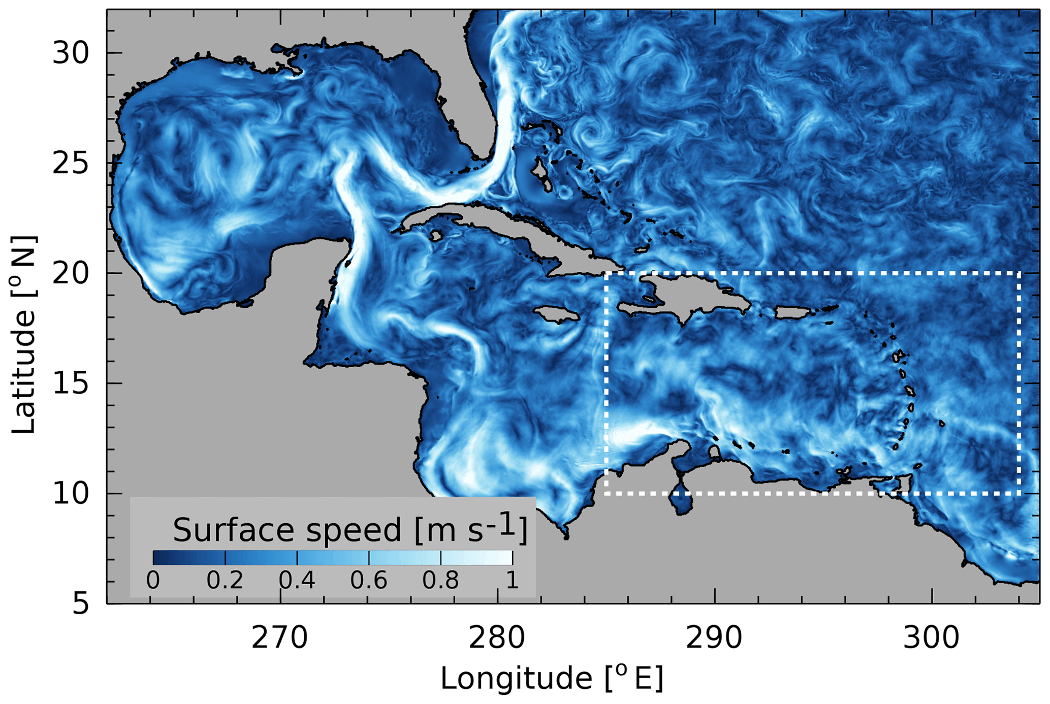
Figure 1AMSEAS model domain. This snapshot of surface currents from the representative date, 2 January 2013, shows prominent features of ocean circulation in the western Atlantic, namely the Loop Current in the Gulf of Mexico and the Florida Current. The rectangular box (dashed white line) indicates the region shown in subsequent plots.
This paper investigates the predictability of sea level associated with the non-phase-locked baroclinic tide in the AMSEAS model, a state-of-the-art operational ocean forecasting system. The emphasis on sea level was chosen (rather than, say, ocean currents) because of its relation to studies of ocean surface topography with satellite altimeters. But even this narrow emphasis poses challenges because of the wide spectrum of non-tidal variability present in sea level. Thus, this study utilizes steric height (which is derived from the forecast model outputs), rather than total sea level, in order to separate the baroclinic tidal signals from broadband high-frequency barotropic variability related to winds and atmospheric pressure. Another challenge for this study is identification of non-phase-locked baroclinic tidal signals in observational data. Neither tide gauge data nor altimeter data permit a unique identification of these signals; and model–data comparisons of high-frequency variability are limited by the AMSEAS output products, which are only available at 3 h intervals. For these reasons, the question of predictability is assessed using self-verifying analyses, where the model output on a subsequent date is used to validate forecasts generated on previous dates. This measure of forecast error thus provides a best-case estimate or lower bound on the forecast skill to be expected with independent data.
Preparation for the Surface Water & Ocean Topography (SWOT) swath altimeter mission, planned for launch in 2021, is concerned with distinguishing balanced motion from inertia–gravity waves in sea surface topography data (Zaron and Rocha, 2018), and the sea surface expression of baroclinic tides is a prominent manifestation of inertia–gravity waves. The present study provides a baseline measure of model forecast skill which will be useful for evaluating future improvements in forecasting baroclinic tides resulting from either changes in the numerical model, the assimilation methodology, or the ocean observation system. The results quantify the forecast skill and provide insight into the phenomenology of internal tide signals as represented in high-resolution ocean models.
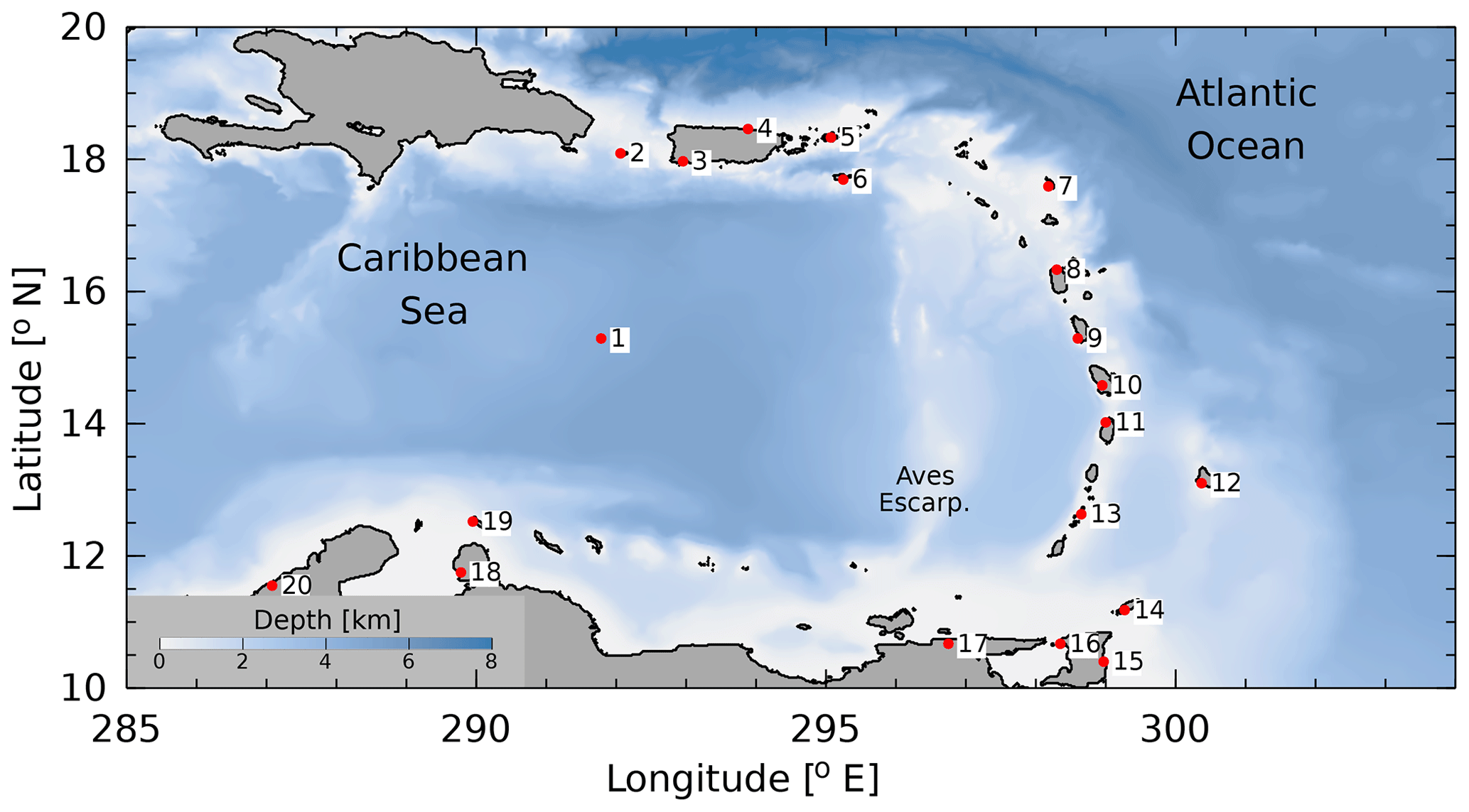
Figure 2Caribbean Sea and tide gauge locations. Tide gauge stations are numbered clockwise around the Caribbean Sea, starting at station 1, DART-42407 (see Table A1). Some closely spaced stations are not plotted. Significant sites of internal tide generation are the Mona Passage (near station 2), Anegada Passage (east of stations 5 and 6), and the passages between the southern Windward Islands (stations 9 to 13) and Grenada Passage (between stations 13 and 17).
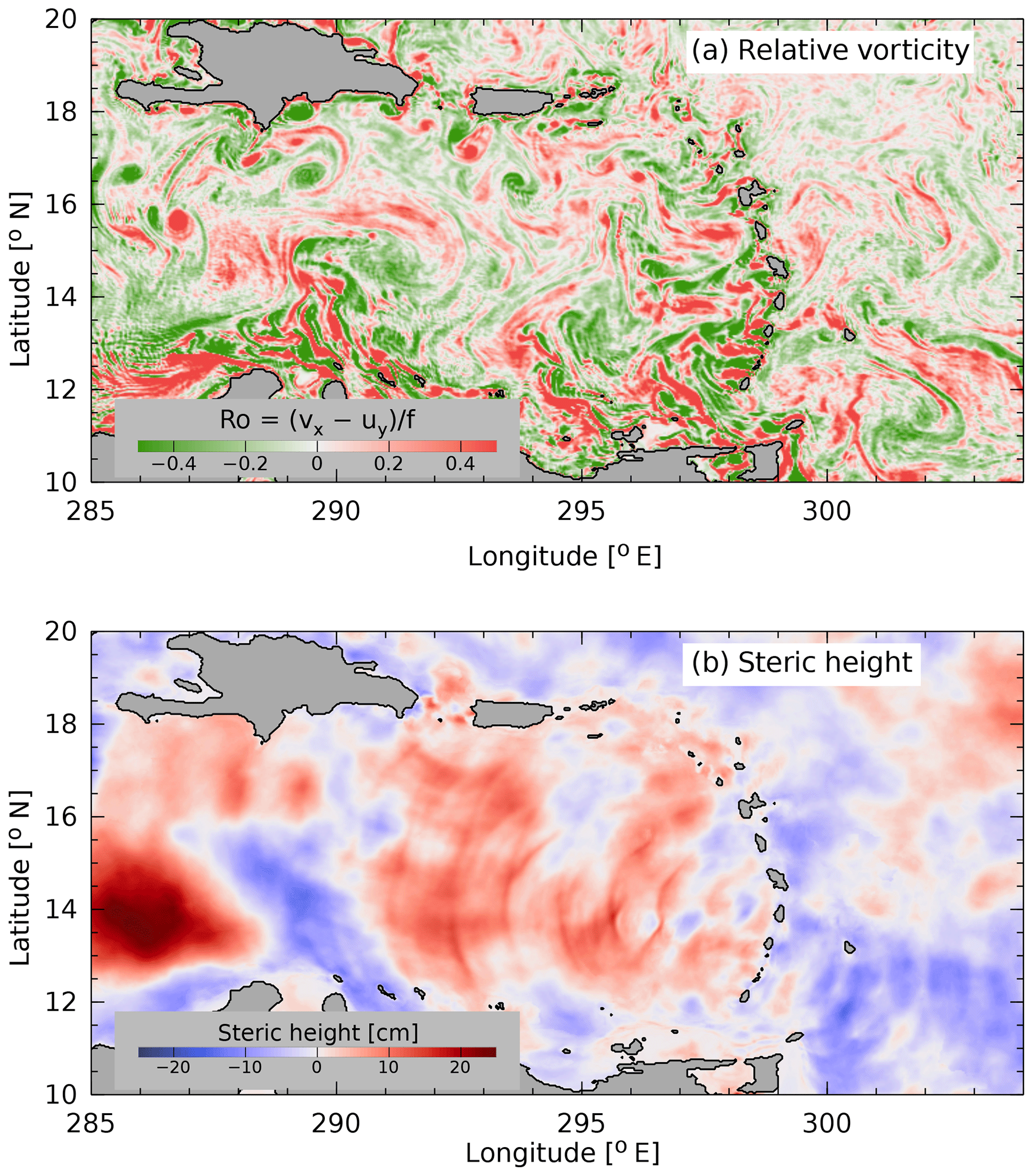
Figure 3Snapshots of AMSEAS model outputs valid on 2 January 2013. (a) The relative vorticity field (expressed as a Rossby number) contains a spectrum of small circular eddies and filamentous structures. (b) Steric height anomaly (relative to the 2-year average).
The AMSEAS model is a 1∕30∘ (approximately 3.5 km), 40-level, implementation of the Navy Coastal Ocean Model (NCOM; Kara et al., 2006) which has been producing operational forecasts of the Caribbean Sea, Gulf of Mexico, and western Atlantic since May 2010. The name, “AMSEAS”, is not an acronym; it is the capitalized contraction of “American seas” which has been adopted as the system's name. The model is re-initialized daily by assimilating observations using the Navy Coupled Ocean Data Assimilation System (NCODA; Cummings, 2011) and integrated to produce a 96 h forecast by the Naval Oceanographic Office (NAVOCEANO). Prior to April 2013, AMSEAS was forced by wind stress and heat flux from the Fleet Numerical Meteorology and Oceanography Center's Navy Operational Global Atmospheric Prediction System (NOGAPS; Rosmond et al., 2002), and lateral open boundary conditions for temperature, salinity, and non-tidal surface elevation were provided by operational global NCOM (Barron et al., 2007). Since April 2013, the atmospheric forcing has been provided by the Navy Global Environmental Model (NAVGEM; Hogan et al., 2014), with lateral boundary conditions provided by operational global HYbrid Coordinate Ocean Model (HYCOM) (Metzger et al., 2014). Tides are not included in the HYCOM presently used for boundary conditions. To incorporate them in AMSEAS, the tides predicted with the Oregon State University (OSU) Tidal Inversion Software (OTIS) barotropic tide model (Egbert and Erofeeva, 2002) are added to the barotropic current and sea surface height data at open boundaries. In addition, a tide-generating force is applied within the model domain which is a combination of astronomical forcing, ocean loading, and ocean self-attraction, consistent with the OTIS model.
The spatial domain of AMSEAS covers the Gulf of Mexico, Caribbean Sea, and a portion of the northeastern Atlantic Ocean (Fig. 1). The major current systems such as the Yucatan Current, Loop Current, and Florida Current are represented in the model, as well as a broad spectrum of variability related to mesoscale eddies, wind-driven circulation, and tides, consistent with historical observations (Carton and Chao, 1999; Centurioni and Niiler, 2003; Torres and Tsimplis, 2011).
AMSEAS nowcast/forecast products have been used and validated in a number of studies. For example, Lagrangian trajectories and forecasts were used to interpret biological observations in the Gulf of Mexico (Nero et al., 2013; O'Conner et al., 2016), and skill assessment efforts in the Gulf of Mexico have been reported (Hernandez et al., 2015; Zaron et al., 2015). AMSEAS was used to provide boundary conditions for a high-resolution regional forecasting system around Puerto Rico and the US Virgin Islands (USVI), and validated through comparisons with tide gauge and water current measurements (Solano et al., 2018).
For later reference, it is useful to refer to Fig. 2 which shows the bottom topography in the region of study. A major topographic feature of the eastern Caribbean, the Aves escarpment, is indicated, as are the locations of 17 tide gauge sites, including one bottom pressure gauge (site 1). Evidence for the range of dynamics active in AMSEAS is shown by the snapshots of the vertical component of relative vorticity at the ocean surface and the steric height in Fig. 3. The relative vorticity field exhibits the attributes of eddies and filaments associated with mesoscale and submesoscale turbulence in the model. The snapshot of steric height exhibits both large-scale features associated with mesoscale eddies, as well as radially coherent features associated with propagating internal gravity waves and, specifically, the baroclinic tide.
The present effort analyzes AMSEAS output from the 2-year period of January 2013–December 2014. For a given date T, AMSEAS produces a nowcast valid at T+0 h, and forecasts every 3 h, up to T+96 h, except for occasional interruptions. The nowcasts and forecasts consist of two-dimensional fields of sea level anomaly (SLA), ηij, as well as three-dimensional fields of temperature, Tijk, and salinity, Sijk, on a fixed longitude–latitude–height grid, .
Identification of phase-locked tidal elevation requires considerable post-processing in order to separate the barotropic and baroclinic SLA components. The SLA output by AMSEAS is the sum of barotropic and baroclinic components, but these components may be separated, approximately, by computing a steric height anomaly from the vertical profiles of temperature and salinity which are also provided by AMSEAS. The steric height anomaly (hereafter referred to simply as the steric height) is defined as
where the density, , is computed using the equation of state of seawater (IOC, SCOR, and IAPSO, 2010), is the time-average density, and is a reference density. The quantity, η′, is the temporal anomaly of the steric height relative to the ocean bottom. Because of simplifications in the dynamics and thermodynamics of NCOM, as well as numerical truncation error (Mellor and Ezer, 1995; Greatbatch et al., 2001), the steric height computed in this manner does not agree precisely with other definitions of the baroclinic sea level, such as might be inferred from projecting the velocity field onto dynamical modes (Wunsch, 2013; Kelly, 2016).
The individual 96 h forecasts produced by AMSEAS are too short for harmonic analysis to produce useful frequency resolution. Instead, the entire 2-year time series is subjected to harmonic analysis to estimate those tides which are phase locked over the entire period. Because any given date/time may contain up to five different estimates for the steric height from the nowcast (T+0 h) and the forecasts (from T+3 to T+96 h in 3 h increments), the harmonic analysis is computed as an unweighted least-squares fit to all the data, including the overlapping forecasts. The following tides are included in the analysis: M2, S2, K2, N2 2N2, K1, O1, P1, and Q1 (provided through tidal open boundary conditions and the tide-generating force) and M3, MS4, M4, and MN4 overtides (generated by the model's nonlinear dynamics). Note that S4 and higher frequencies may be present in the model, but they are aliased by the 3 h time sampling.
A detailed comparison between the modeled and observed phase-locked M2 and K1 tides at the sites indicated in Fig. 2 is provided in Appendix A. The main features of the observed tide are reproduced in the model. These include a counter-clockwise propagation of the M2 tide around an amphidrome in the northeast Caribbean and standing-wave-like behavior of K1, exhibiting maximum amplitude of about 10 cm along the South American coast (Kjerfve, 1981; Torres and Tsimplis, 2011).

Figure 4Internal tide along Jason-1 track no. 191. The in-phase component of the high-passed M2 tide has maximum peak-to-peak amplitude of 1.5 cm in AMSEAS (dashed) and slightly larger amplitude in the altimeter data (solid). Alignment of peaks and troughs is good, particularly near the apparent generation site, Mona Passage, west of Puerto Rico (inset).
The curvature of the wave-like features in Fig. 3b suggests that the baroclinic tide is generated at a relatively small number of sites, namely, at Mona Passage between the Dominican Republic and Puerto Rico (18∘ N, 292∘ E), and along the southern Windward Islands (14∘ N, 298∘ E; see caption of Fig. 2). Satellite altimeter ground tracks are not dense enough to map the baroclinic tides accurately in the Caribbean; however, the signals are unmistakable along individual tracks. Figure 4 compares the in-phase component of the M2 tide in AMSEAS with the same quantity inferred from altimetry along a track which passes south of Mona Passage. The peaks and troughs are roughly aligned in the model and observations, and the amplitudes of the waves are quite similar in the mid-basin, although the values certainly differ in detail.

Figure 5Forecast decomposition and errors for the date, 4 January 2013. For the purpose of analysis, the steric height forecast is decomposed into a sum of three components: (a) low-frequency (24 h average), (b) phase-locked tide, and (c) high-frequency (residual). The forecast error is defined as the forecast minus the verifying analysis, valid at the same time. The two components of the forecast error are (d) the low-frequency component and (e) the high-frequency component; the phase-locked tide is identical in the forecast and the analysis. Note the different color scales shown for the high- and low-frequency components.
The calibration of AMSEAS to improve its representation of baroclinic tides has not been attempted, and the effort involved in such a task would be substantial as it pertains to both the model itself and the choice of appropriate observational data. For example, it is likely that further refinement of the resolution of AMSEAS would improve the representation of the phase-locked tide. While the baroclinic tide SLA field is predominantly a mode-1 phenomena, with wavelength in excess of 100 km, achieving quantitative accuracy depends on resolving the detailed seafloor topography of the generation sites; based on experience modeling other sites, this requires a horizontal resolution of 1–2 km (Zaron and Egbert, 2006; Guihou et al., 2017; Aslam et al., 2018). Furthermore, the distinction between barotropic and baroclinic sea level is unambiguous in the model, but this same distinction cannot be made with most observations, such as altimetry, so calibration efforts would need to contend with the ambiguous attribution of model–data differences to barotropic, baroclinic, and non-tidal processes, as well as measurement noise. Non-phase-locked tidal variability may also contribute to the differences between the model and observations but to a degree which is presently unknown. Appendix A contains a graphical comparison of AMSEAS tides versus those inferred from altimetry.
The above remarks concerning the challenges of calibrating AMSEAS motivate the methodology used to assess the forecast error of non-phase-locked tides in AMSEAS. In the nomenclature of numerical weather forecasting, the approach taken is a self-analysis verification or self-verification (e.g., Privé and Errico, 2015). The forecast error is measured by comparing the nowcast valid at date, Tn, with a forecast previously computed on the date, , with a given lead time, τ, i.e., . This approach may be contrasted with a forecast verification based on independent observations, in which the forecast and observations are compared directly as the latter become available. The self-verification is likely to lead to an optimistic estimate of the forecast error; nonetheless, it appears to be the only feasible approach to assessing the predictability of the non-phase-locked tide at present. The reasons for using the self-verification have more to do with the available data rather than the forecast system, since there are no data which can reliably distinguish non-phase-locked and phase-locked tidal variability over the timescales and space scales represented within the AMSEAS forecasts.
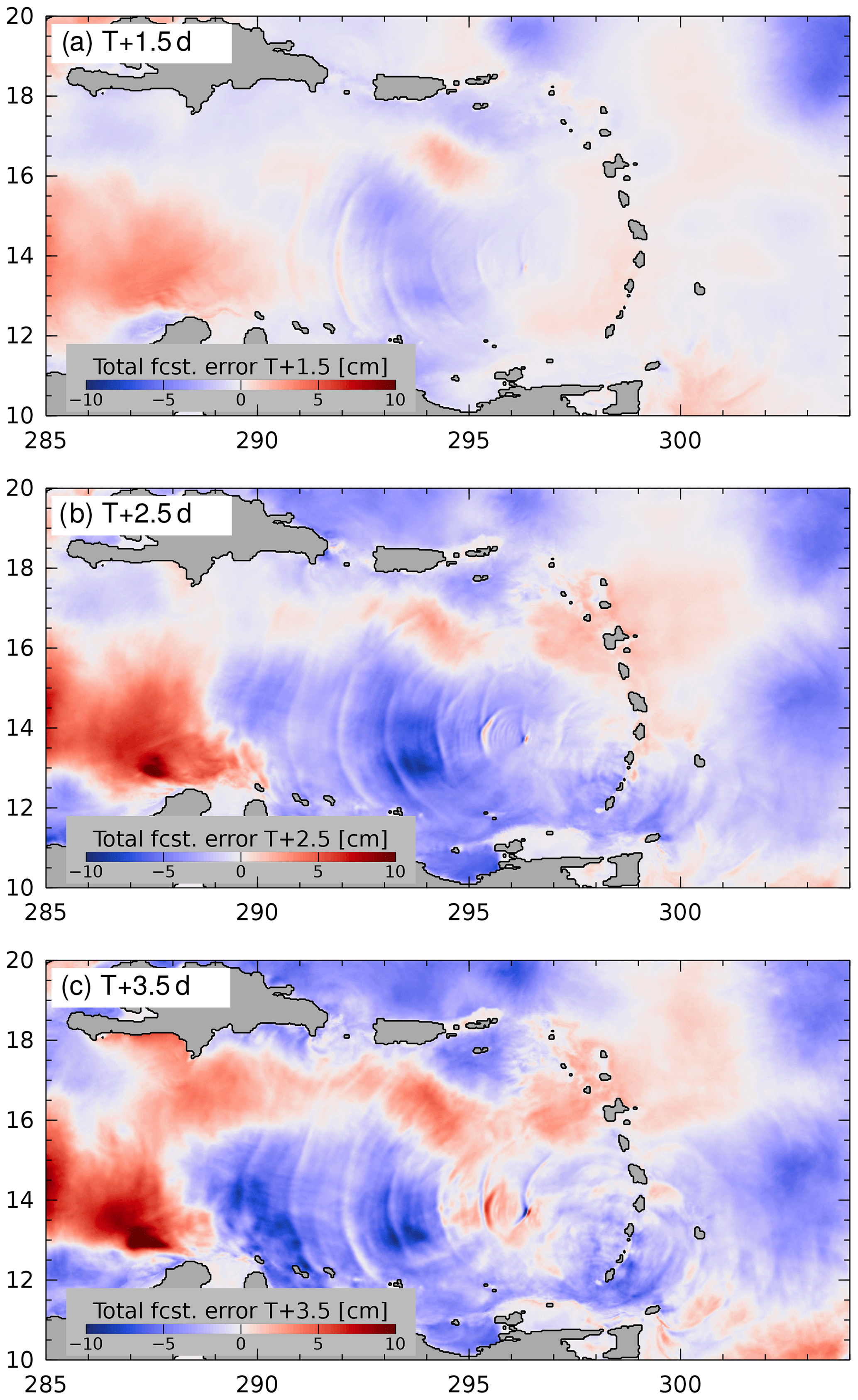
Figure 6The steric height forecast error for different lead times for Tn= 4 January 2013 at 12:00:00 Z: (a) d, (b) d, and (c) d. Note that the color scale differs from previous figures; it was chosen to make the error growth visible as a function of increasing forecast lead time.
The previous section focused on the phase-locked tide, the unambiguous definition of which is provided by harmonic analysis and the constant phase with respect to the known astronomical tidal potential. In contrast, the definition of the non-phase-locked tide is potentially ambiguous since it involves distinguishing tide-band and non-tidal variability, which implicitly requires either a dynamical definition or a definition based on frequency bandwidth. In addition, a bandwidth-based definition must be meaningful within the available duration of each forecast, which is only 4 d (from T+0 to T+96 h). The challenge, then, is to develop a decomposition which can diagnose the non-phase-locked tide from a small number of snapshots of the steric height (e.g., Fig. 3b).
An example of such a decomposition is presented in Fig. 5, in which the steric height is represented as the sum of a low-frequency component (Fig. 5a), a phase-locked tidal component (Fig. 5b), and a high-frequency component (Fig. 5c). The high-frequency component, which shall be identified with the non-phase-locked tide, is simply computed as the residual of total steric height, minus the predicted phase-locked tide, minus the low-frequency 24 h-average steric height. More tersely, the non-phase-locked tide is defined as the anomaly of steric height with respect to the daily average of the de-tided steric height. To compute this quantity, a tidal prediction is created using the complex harmonic constants for the 13 astronomically forced and compound tides described previously, and this predicted tide is removed from the steric height. Then, the daily average of the de-tided steric height is computed centered at noon of each forecast day (T+12, T+36, T+60, and T+84 h) to provide an estimate of the low-frequency steric height field.

Figure 7Zonal transect of temperature at 13.7∘ N (cf. Fig. 5). (a) The high-frequency (HF) temperature forecast and (b) the HF verifying analysis, both valid at 4 January 2013 at 12:00:00 Z. The solid contours indicate the total temperature field (2 ∘C contour interval). The dashed line at the top, centered on z=0, is the HF steric height in units of millimeters (the maximum at E is almost ). This transect cuts slightly north of the shallow seamount, Aves Ridge, which rises to within about 600 m of the ocean surface at 13.4∘ N, 297∘ E. Here, the topography is represented by the gray shading visible near 297, 299, and 300∘ E. (c) The HF forecast temperature error (color scale) and steric height error (dashed line centered at z=0) are largely associated with a slight shift in the location of the wave at 296.1∘ E. (d) Error in the low-frequency (LF) forecast is represented with error in buoyancy frequency, N(z), which is multiplied here by 200 m to scale it like mode-1 baroclinic wave phase speed (based on the Wentzel–Kramers–Brillouin (WKB) approximation, , about 3 m s−1). Contours represent LF temperature error (0.5 ∘C contour interval, positive in black, negative in red) with thicker contours at +0.75 and C.
This methodology provides a pragmatic definition of the non-phase-locked tidal steric height valid at T+12, T+36, T+60, and T+84 h. Alternative approaches could be envisioned, perhaps involving band-pass filtering or complex demodulation, but they would be problematic due to phase errors near the start and end of the 4 d forecast windows. The present approach is relatively simple to implement and explain, and it unambiguously partitions the steric height variance between the low-frequency motion, phase-locked tides, and high-frequency processes, the latter being dominated by non-phase-locked tides (as may be verified a posteriori, e.g., Fig. 10).
The fields centered at T+12 h shall be regarded as the verifying analyses (nowcast) which are to be compared with the forecasts from three previous days at , , and . To shorten the notation, forecasts at these lead times will be denoted with the time offset in days, as “T+1.5”, “T+2.5”, and “T+3.5”, in subsequent figures.

Figure 8Root mean square (rms) quantities valid at Tf+3.5 d (panel layout corresponds to snapshots in Fig. 5): (a) low-frequency forecast, (b) phase-locked tide forecast, and (c) high-frequency forecast; and the corresponding errors: (d) low-frequency forecast error and (e) high-frequency forecast error. Note the different color scales used for low-frequency variability. The “spectral analysis domain” in panel (d) indicates the region used for the computation of the radial wavenumber spectra in Fig. 10, below; it is also the region of spatial averaging for the forecast errors summarized in Fig. 9.

Figure 9High-frequency (HF) forecast error. (a) HF forecast error is an increasing function of LF forecast error, and error increases as a function of lead time (T+1.5 d shown in red, T+3.5 d shown in black). (b) HF forecast error depends weakly on the phase-locked tide (red and black dots as in panel a).
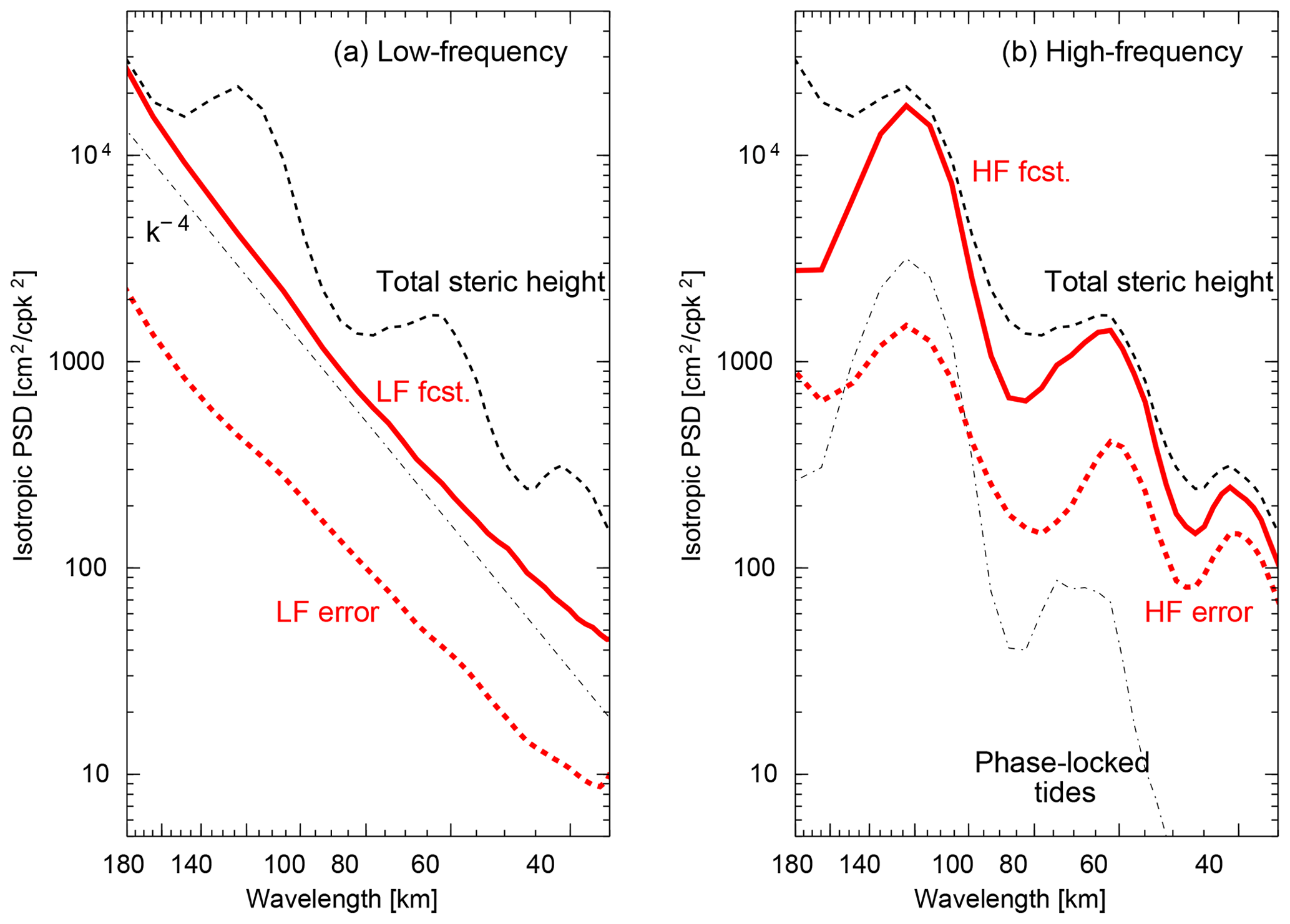
Figure 10Isotropic wavenumber power spectral density for (a) low-frequency and (b) high-frequency steric height components. The k−4 wavenumber dependence (dash–dot black line) is shown for reference in panel (a); the spectrum of the phase-locked tides (dash–dot black line, a component of the HF forecast) is shown for reference in panel (b); and the total steric height spectrum is repeated in both panels (dashed black line). The LF error (dashed red line, panel a) is approximately a constant fraction of the LF forecast (solid red line) independent of scale. In contrast, the HF error (dashed red line, panel b) is an increasing fraction of the HF forecast (solid red line) as wavelength decreases.
The decomposition of the steric height field just described is illustrated in Fig. 5 for the representative date, 4 January 2013. The low-frequency component of the forecast steric height (Fig. 5a) resembles a spatially smoothed version of the snapshot shown previously (Fig. 3b), but it is obtained by temporal, not spatial, averaging. The small-scale waves in Fig. 3b are the sum of the predicted tide (Fig. 5b) plus the high-frequency residual (Fig. 5c). The panels in the left column of Fig. 5 are valid on T= 4 Januray 2013 at 12:00:00 Z, but they were forecast 3.5 d prior on 1 January 2013 at 00:00:00 Z; the right panels show the errors in the forecasts, computed by subtracting the nowcast at Tn=T. The low-frequency error field (Fig. 5d) is relatively smooth and takes on largest values in the southeast, near the edge of the continental shelf where strong currents are present (13∘ N, 287∘ E; cf. Fig. 1). The error in the high-frequency component of the steric height (Fig. 5e) exhibits wavelike features. For this particular date, it is clear that the magnitudes of the forecast error fields (right panels) are smaller than the forecasts themselves (left panels); however, the error fields are non-random and display the features one might associate with difficult-to-forecast components of the flow field, e.g., small scales and high-current zones. Note that the range of steric heights shown in Fig. 5a and d is different from that used in the other panels of Fig. 5.
To illustrate the character of the forecast errors as a function of increasing lead time, τ, Fig. 6 shows the sum of the low- and high-frequency steric height errors for three lead times, and 3.5 d, valid on the same date as above. The steric height signal associated with mesoscale features is in the range of ±15 cm, which is much larger than the typical range, ±5 cm, associated with the baroclinic tide. The magnitude of the forecast error associated with the low-frequency flow is somewhat larger than the magnitude of the error associated with the high-frequency flow (cf. Fig. 5d and e), but their increase in time is evident in Fig. 6.
Forecast errors of the low- and high-frequency steric height components exhibit different dynamical features. The most striking qualitative features of the high-frequency forecast and the high-frequency error (Fig. 5c and e) are spatially coherent wave trains. Note that the peak amplitudes of both the low- and high-frequency forecasts are considerably larger than the error fields; thus, the model apparently captures much of the low-frequency variability that modulates the high frequencies. The high-frequency error field is associated with small scales, and in Fig. 5e it exhibits wavefronts which appear to radiate from the Aves escarpment (13.5∘ N, 296∘ E) and the west side of Mona Passage (18∘ N, 291∘ E). To gain some insight into the oceanographic processes leading to these forecast errors, Fig. 7 shows transects of high-frequency temperature (Fig. 7a–c) and low-frequency Brunt–Väisälä frequency anomaly (Fig. 7d). The high-frequency steric height along this section exhibits a wave with nearly 10 cm amplitude at 296∘ E, in both the forecast and the verifying analysis (Fig. 7a, b). The error field (Fig. 7c) shows that this feature is slightly offset in the analysis and forecast; however, the sawtooth shape of the steric height waveform leads to an error field with nearly the same peak amplitude as in the forecast. This appears to be a mode-1 internal wave which has steepened considerably, possibly during its passage over the Aves Ridge. The error in the low-frequency forecast (Fig. 7d), expressed in terms of the error in the buoyancy frequency, N(z), is not pronounced over the ridge; rather, it displays a broad positive anomaly at about 150 m depth and a negative anomaly at the base of the surface mixed layer.
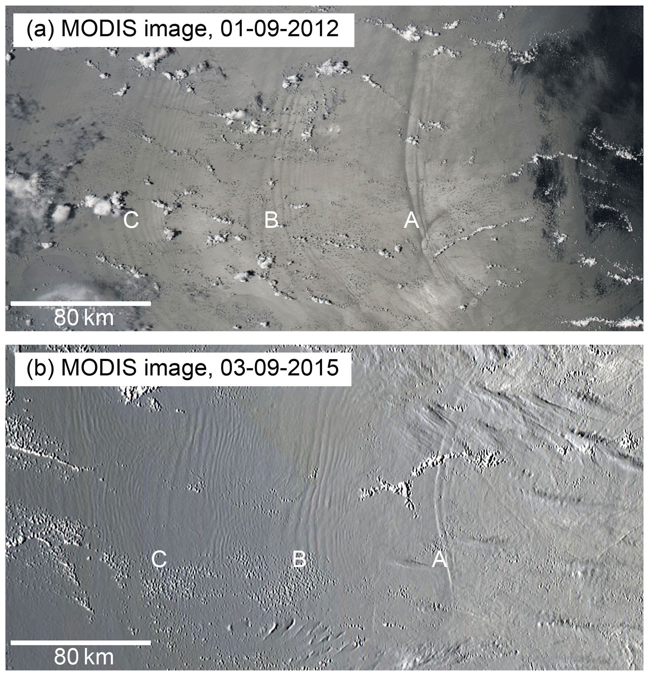
Figure 11Internal wave packets in MODIS imagery from the Aves escarpment. MODIS Sun-glint imagery from dates in (a) 2012 and (b) 2015 (digitally enhanced) exhibits the surface expression of three packets of internal waves, at longitudes marked A, B, and C. Remarkably, similar wave packets are visible in imagery from 5 September 2018 (not shown). The largest packet, A, is located at Aves Ridge ( N, E) on the Aves escarpment.
Given the above decomposition of the nowcast/forecast steric height fields, the statistics of the forecast errors have been computed for the 2-year period of 2013–2014.
A summary of the spatial statistics is provided in Fig. 8, which shows the rms of the different steric height components, corresponding to the panels in Fig. 5. The low-frequency forecast (Fig. 8a) and its error (Fig. 8d) are spatially uniform except for the influence of water depth on steric height variability. The spatial distributions of the phase-locked (Fig. 8b) and non-phase-locked tides differ (Fig. 8c); the amplitude of the phase-locked tide is largest near its sources in the Mona Passage and near the Windward Islands, while the non-phase-locked tide is largest around the Aves escarpment, some distance from the wave source. The high-frequency forecast error (Fig. 8e) is spatially uniform, except near the Aves Ridge. This pattern might be explained by statistically homogeneous refraction of the internal tide by the mesoscales, except in the vicinity of the Aves Ridge, where the internal tide generated near the Windward Islands is focused (Fig. 8b, c), and where sawtooth-shaped (nonlinear) wave profiles were noted above (cf. Fig. 7).
Because the non-phase-locked tide arises as a consequence of the time-variable propagation medium, it was hypothesized that the forecast error for the non-phase-locked tide would be related to the forecast error for the low-frequency flow. This hypothesis is generally confirmed by the statistics in Fig. 9a, which shows the high-frequency error as a function of the low-frequency error. The forecast errors for the two components of the steric height are positively correlated (note that the errors reported here are rms averages over the domain denoted “spectral analysis domain” in Fig. 8d); however, there is considerable scatter in the high-frequency error which is unrelated to the low-frequency error. A plot of the forecast error versus the amplitude of the phase-locked tide (Fig. 9b) indicates that the error is only weakly dependent on the phase-locked tide (e.g., the spring–neap cycle). The scatter of the high-frequency error with respect to these rms statistics is consistent with the genesis of the errors at small-scale features which are inherently less predictable and constrained by observations. Note that the errors for the T+3.5 d forecasts (black dots) are larger than for the T+1.5 d forecasts (red dots), as would be expected (cf. Fig. 6).

Figure 12Fraction of variance: phase-locked versus total high-frequency variance (phase-locked plus non-phase-locked variance).
A spectral analysis of the steric height anomaly has been conducted in order to understand the scale dependence of the forecast error. The isotropic power spectral density shown in Fig. 10, equal to (2πk)−1 times the azimuthally averaged 2-D power spectrum (within the “spectral analysis domain” indicated in Fig. 8d), clearly exhibits peaks related to the baroclinic tide.
The tidal peaks are completely absent in the low-frequency forecast and its error (solid and dashed red, respectively, in Fig. 10a). In contrast, the tidal peaks dominate the spectra of the high-frequency steric height (Fig. 10b). The variance associated with the mode-1 semi-diurnal baroclinic tide, at a wavelength of 120 km, is partly associated with the predictable phase-locked tide (dash–dot black line), and the forecast error (dashed red line) is less than 10 % of the total high-frequency forecast variance (solid red line). At wavelengths shorter than the mode-1 wave, the high-frequency forecast error is larger than the phase-locked tide and it is a larger fraction of the total high-frequency variance. In other words, as would be expected, the baroclinic tides are increasingly less phase locked, and less predictable, at smaller scales.
The results of this study provide a descriptive snapshot of AMSEAS forecast skill during one 2-year period, and they are presumably dependent upon the particular ocean observing system, numerical model resolution and configuration, and data assimilation algorithm used during this period. Nonetheless, the results provide some insight into the capabilities and limitations of such a system for predicting and explaining high-frequency ocean variability. For example, it is evident in Fig. 10b that the wavelength peak associated with the mode-2 phase-locked tides (dash–dot black line) occurs at a slightly longer wavelength than the nearby peaks in either the high-frequency forecast (red line) or the forecast error (dashed red line). In fact, an examination of the model output (not shown) indicates that the high-frequency forecast and forecast error associated with the 60 km wavelength peak are related to the nonlinear mode-1 baroclinic tide generated on the shoals of the Aves escarpment, while the 70 km peak in the phase-locked tide is related to the mode-2 baroclinic tide. The nonlinear mode-1 dynamics may be AMSEAS' rendition of the internal wave packets generated along the Aves escarpment which have been identified in satellite Sun-glint imagery (Alfonso-Sosa, 2013) and are the cause of coastal seiches around Puerto Rico (Giese et al., 1990; Alfonso-Sosa, 2015; Woodworth, 2017), nearly 1000 km to the northwest. Figure 10b indicates that a considerable fraction of the variance associated with the wavenumber peak near 60 km is predictable by the AMSEAS system, even though is it not phase locked with the astronomical tidal forcing. Indeed, a brief search of the MODIS Sun-glint imagery found the pair of images displayed in Fig. 11 in which similar wave packets are found in images taken 3 years apart. These images provide evidence of nonlinear internal waves too small to be directly resolved by AMSEAS; however, their recurring pattern is certainly suggestive of some degree of predictability.
A dedicated study of the dynamics responsible for both the predictable and unpredictable high-frequency variability would be needed to understand the factors responsible for the time-variable propagation of the baroclinic tide and its generation. The high-frequency forecast error is correlated with the low-frequency forecast error (Fig. 9), but the reason for this correlation has not been examined in detail. It was initially hypothesized that errors in location or intensity of (low-frequency) forecast mesoscale eddies would be the cause of errors in the high-frequency forecasts; however, there are other possible explanations for this relationship. For example, the generation of higher baroclinic modes and nonlinear overtides near the Aves Ridge probably depends on the near-surface stratification at this site, and there are many factors which might influence this aside from the location of mesoscale eddies. Another explanation for the correlated errors is related to how the observed SLA data are assimilated with the NCODA system, which projects the observations onto subsurface profiles of temperature and salinity. The presence of non-phase-locked tidal signals in the observations might be erroneously attributed to mesoscale features and assimilated into the model; in this case, the low-frequency error would be caused by the high-frequency variability, rather than vice versa.
Efforts to map the baroclinic tide with satellite altimeter data are generally only capable of identifying the phase-locked part of the tidal signals (Ray and Mitchum, 1996; Carrère et al., 2004). Attempts to quantify the energy transport, and dissipation, of the baroclinic tide from altimetry data must make assumptions about the partitioning of energy between the phase-locked and non-phase-locked tides; however, present estimates for non-phase-locked tidal steric height suffer from sampling limitations (Zilberman et al., 2011; Kelly et al., 2015; Zaron, 2015, 2017). Ocean models are increasingly being used to study this quantity (Shriver et al., 2014; Kerry et al., 2016; Savage et al., 2017; Ansong et al., 2017), and AMSEAS is presently one of the highest-resolution models which includes both tides and wind-driven circulation. The ratio of phase-locked to total high-frequency steric height variance shown in Fig. 12 indicates that the phase-locked tide dominates the variance – hence energy – only within a few hundred kilometers of the generation sites in the Caribbean Sea. The baroclinic tide in the middle of the Caribbean Sea is dominated by the non-phase-locked component. Whether or not this result is more broadly applicable is unknown, but the variance fraction is a useful diagnostic of the partition between open-ocean versus boundary dissipation of the baroclinic tide (Zaron, 2019).
Finally, an important caveat with the present study is related to the use of self-verifying analyses to assess the forecast errors. This approach is capable of measuring the predictability of the high-frequency steric height only to the extent that AMSEAS accurately represents the ocean dynamics. This approach is not capable of identifying systematic errors shared by the analysis and the forecast (e.g., errors in the phase-locked tides) and it thus provides a lower bound on the actual forecast error. To estimate this quantity, consider the rms goodness of fit to the assimilated SLA, which is roughly σ=6 cm (Zaron et al., 2015). Assuming this value is the sum of independent components of instrumental measurement error, σe=3 cm; baroclinic tide signal, σt=4 cm (treated as “representation error” in the NCODA assimilation); and unknown analysis error, σa; one may use to estimate σa=3 cm. This is a lower bound for the analysis error at the measurement sites, as it does not account for the larger error between the satellite ground tracks. If σa=3 cm is taken as the lower bound on the low-frequency forecast error, then Fig. 9 suggests that 0.75 cm is a lower bound on the high-frequency forecast error. This is a crude estimate which does not account for the geographic variability of either the ocean dynamics or the ocean observing system, but it provides a guide to the best case which may be attained in practice.
This study has examined the predictability of non-phase-locked baroclinic tides using 4 d ocean forecast products from the AMSEAS system. It was motivated by the desire to understand our present capability for predicting baroclinic tidal SLA, which is expected to be a key limitation for measuring mesoscale and submesoscale processes with the forthcoming SWOT wide-swath satellite altimeter (Callies and Wu, 2019). The AMSEAS system is well suited to this task since it represents the state of the art among data-assimilating ocean forecast systems; it has resolution sufficient to realistically represent baroclinic tide generation and propagation, and the 4 d forecast cycle is adequate to separate the SLA signals of low-frequency balanced motions from high-frequency processes, the latter being dominated by baroclinic tides.
The findings of this study indicate that a substantial fraction of non-phase-locked tidal sea level variability may be predictable with an ocean forecasting system. This result has been demonstrated using self-verifying analyses with the AMSEAS system, and future studies should investigate how to use independent high-frequency data to verify forecast skill statistics. The small-scale and spatial inhomogeneity of the baroclinic tide makes this a challenging task. Nonetheless, many applications of altimetry which regard the tidal SLA as noise would benefit from improved predictions of baroclinic tidal sea level.
The software and data products used in this research are available from the author.
A1 Tide gauges
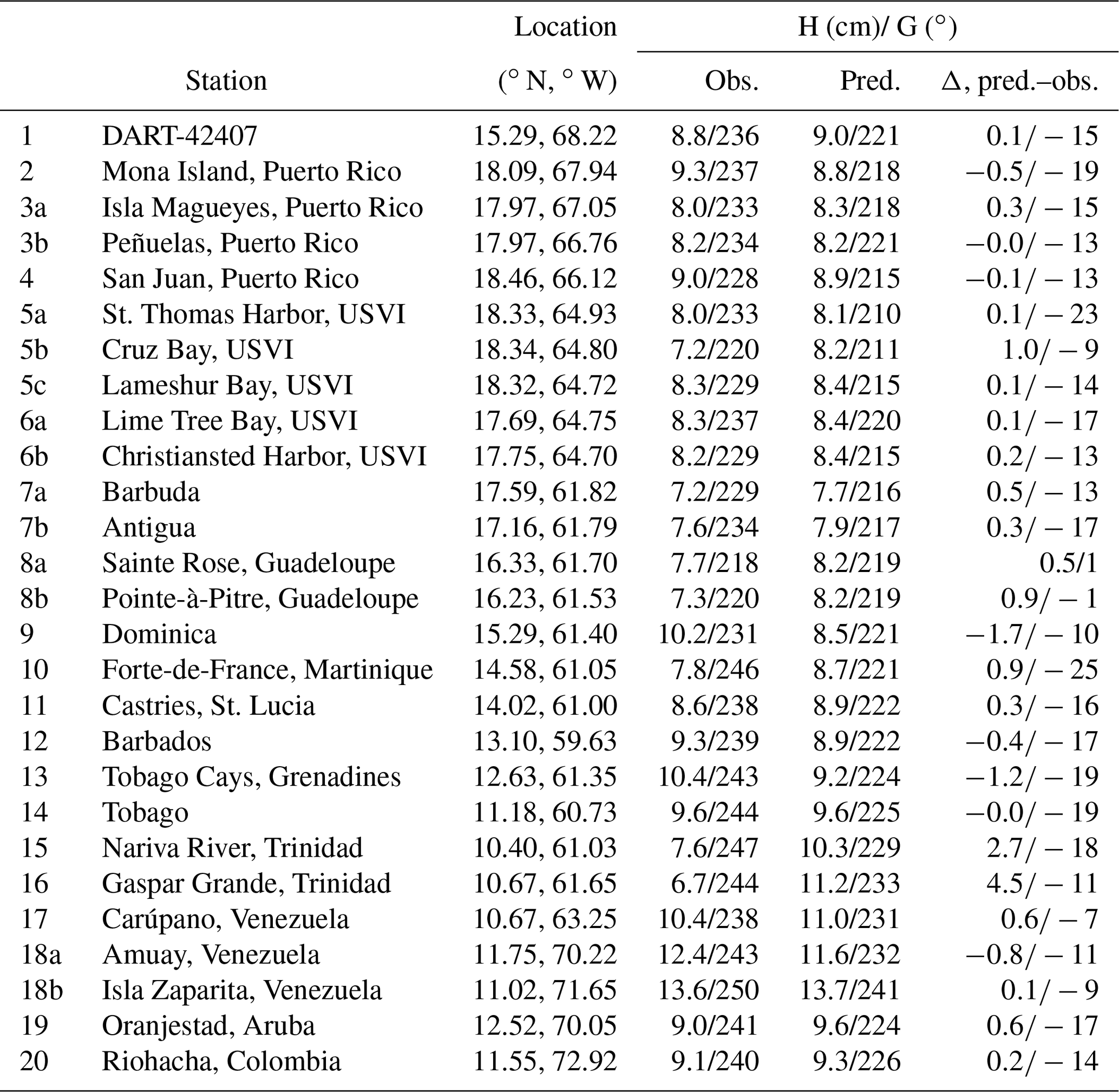
Tables A1 and A2 provide quantitative comparisons of the phase-locked tide sea surface height at tide gauges (and one bottom pressure sensor, DART-42407) in the Caribbean Sea for the main semi-diurnal and diurnal tides, M2 and K1. The observed data come from three sources: the National Data Buoy Center (for the DART buoy), the NOAA Center for Operational Oceanographic Products, and historical stations in Kjerfve (1981), as indicated in Table A1.
The amplitude and Greenwich phase lag of the observed (obs.) and predicted (pred.) AMSEAS sea surface heights are listed. The station number in the first column corresponds to the location in Fig. 2. Stations located too close to distinguish on the map are indicated with lowercase letters in the tables, e.g., “7a Barbuda” and “7b Antigua”.
Overall, the observed and predicted tides agree within a centimeter or two at most stations, with a few interesting exceptions. Because tides are relatively small in the Caribbean, the M2 fractional errors are large, particularly in the northeast (e.g., stations 3, 5, and 6), near the M2 amphidromic point (Kjerfve, 1981). Because the tide gauge measurements cannot distinguish barotropic and baroclinic sea level, it may be that much of the error can be attributed to small-scale differences in the baroclinic tide. The amplitude errors for K1 are small, less than a centimeter almost everywhere, but a widespread phase error is present, except, oddly, at stations 8a and 8b on Guadeloupe. The reason for the K1 phase error is obscure, but it may be related to the fact that K1 behaves like a standing wave, so its phase may be strongly influenced by wave reflection at both open boundaries and the coastline in the AMSEAS model.
Table A1Tide gauge stations and tidal statistics: M2.
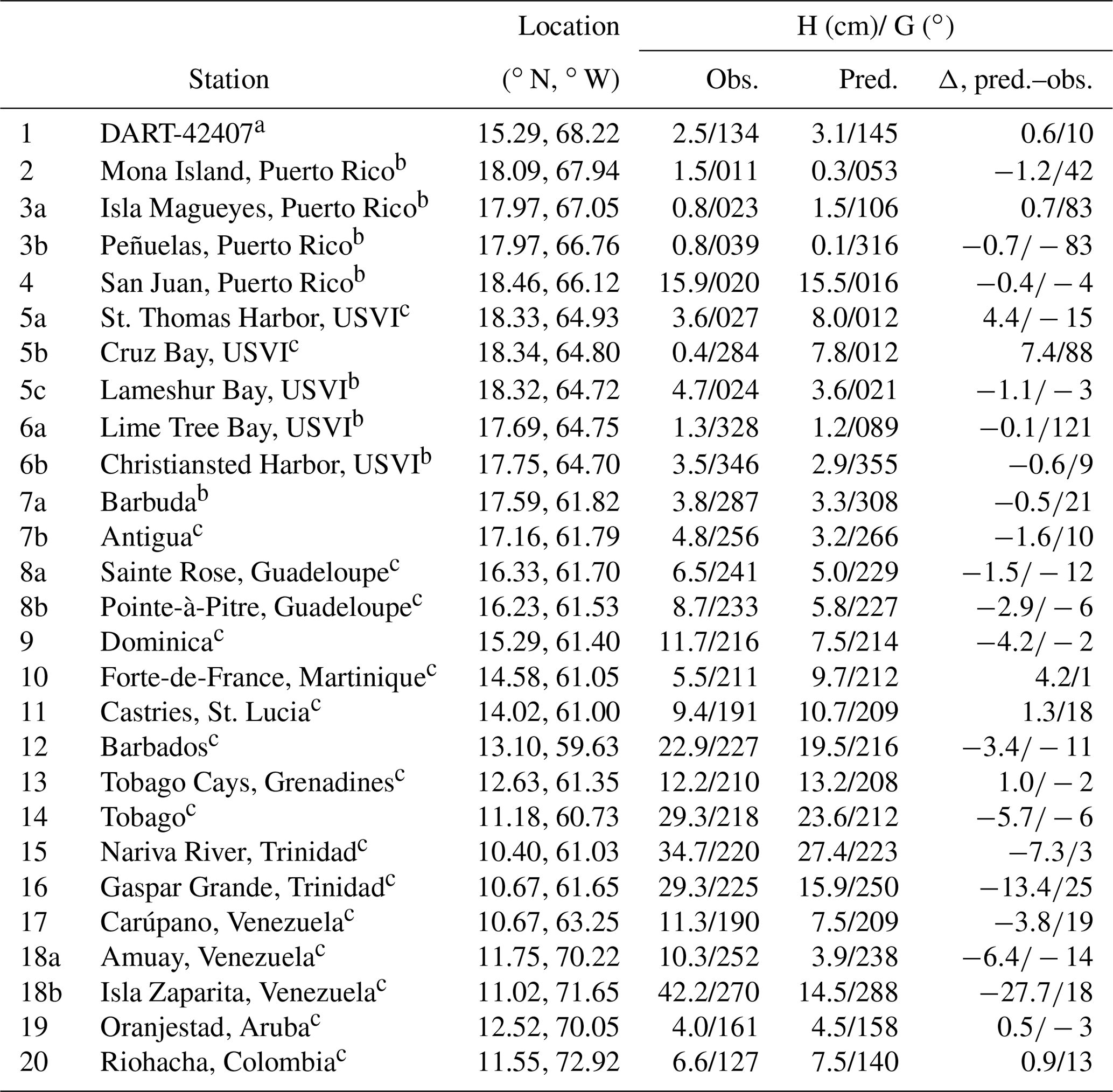
a National Data Buoy Center, station 42407; http://www.ndbc.noaa.gov (last access: 27 September 2019). b NOAA Center for Operational Oceanographic Products and Services; http://tidesandcurrents.noaa.gov (last access: 27 September 2019). c Kjerfve (1981).
A2 Satellite altimetry
A graphical comparison of AMSEAS and altimeter-derived tides is provided in Figs. A1 and A2. The M2 tide was estimated from TOPEX/Poseidon (thin black line) and Jason-1 (thin blue line) altimetry data for the periods 1992–2002 and 2002–2009, respectively, while the AMSEAS phase-locked tide was computed as described in Sect. 3 of the main text.
There are two primary inferences to be drawn from the comparisons. The first pertains to the data; namely, there are differences in the harmonic constants estimated from the TOPEX/Poseidon and Jason-1 data. It is not clear at present whether these differences are caused by long-term trends and interannual variability of the tides (e.g., Müller, 2011; Devlin et al., 2017) or by noise related to mesoscale variability (e.g., Ray and Byrne, 2010). Differences in the tide are at the level of roughly 2 cm in a few regions (Fig. A1c at 14∘, Fig. A1d at 16∘ N) but they are generally 1 cm or less. The directional character of the baroclinic waves and relatively small size of the Caribbean makes it challenging to use along-track filtering to isolate the barotropic and baroclinic components of tidal sea level. The second pertains to the model; namely, there are apparently no gross differences between the observed and modeled tide, at least for M2 (shown) and other large tides which have been examined (K1 and O1; not shown). However, the tidal amplitudes are small enough that even a 1 cm difference in amplitude is a significant fraction of the total amplitude.
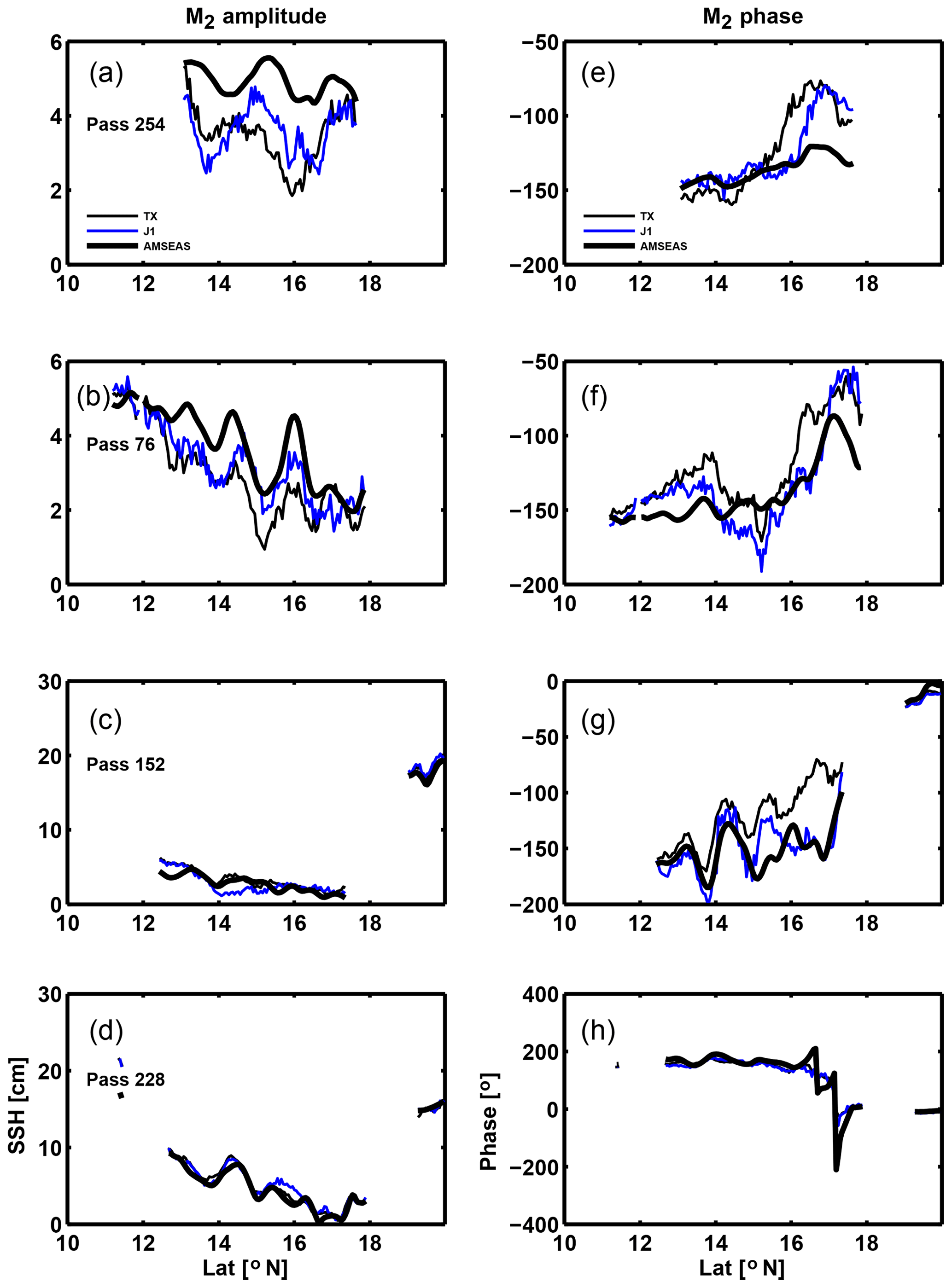
Figure A1Comparison of satellite-derived and AMSEAS phase-locked tides in the Caribbean Sea: descending tracks.
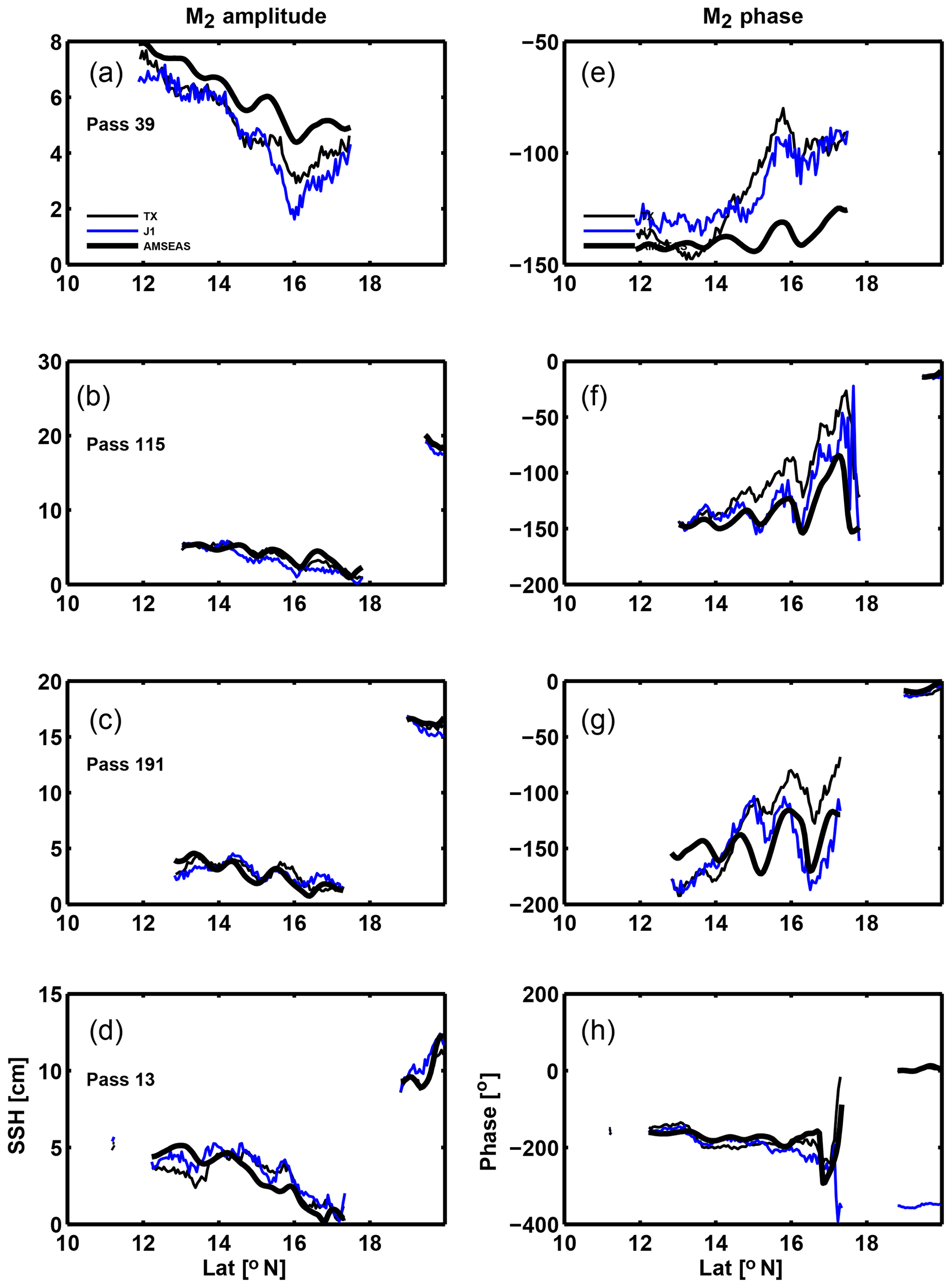
Figure A2Comparison of satellite-derived and AMSEAS phase-locked tides in the Caribbean Sea: ascending tracks.
The author declares that there is no conflict of interest.
This article is part of the special issue “Developments in the science and history of tides (OS/ACP/HGSS/NPG/SE inter-journal SI)”. It is not associated with a conference.
Three anonymous reviewers and the editor are acknowledged for their contributions to improving the manuscript. AMSEAS model products are created by NAVOCEANO and distributed in cooperation with the Northern Gulf Institute; they are available at http://edac-dap.northerngulfinstitute.org/ (last access: 27 September 2019). Satellite altimeter data were extracted from the Radar Altimetry Database System (RADS), available at http://rads.tudelft.nl/rads/rads.shtml (last access: 27 September 2019). This work was supported by NASA awards NNX17AJ35G and NNX16AH88G.
This research has been supported by the National Aeronautics and Space Administration (grant nos. NNX17AJ35G and NNX16AH88G).
This paper was edited by Philip Woodworth and reviewed by three anonymous referees.
Alfonso-Sosa, E.: First MODIS Images Catalog of Aves Ridge Solitons in the Caribbean Sea (2008-2013), working notes published on the author's web site, 33 pages, available at: https://www.academia.edu/5500852/First_MODIS_Images_Catalog_of_Aves_Ridge_Solitons_in_the_Caribbean_Sea_2008-2013, (last access: 27 September 2019), 2013. a
Alfonso-Sosa, E.: Seiches Costeros de Puerto Rico, Ocean Physics Education, Puerto Rico, 2015. a
Ansong, J. K., Arbic, B. K., Alford, M. H., Buijsman, M. C., Shriver, J. F., Zhao, Z., Richman, J. G., Simmons, H. L., Timko, P. G., Wallcraft, A. J., and Zamudio, L.: Semidiurnal internal tide energy fluxes and their variability in a global ocean model and moored observations, J. Geophys. Res., 122, 1882–1900, 2017. a
Aslam, T., Hall, R. A., and Dye, S. T.: Internal tides in a dendritic submarine canyon, Prog. Oceanogr., 169, 20–32, 2018. a
Barron, C. N., Kara, A. B., Rhodes, R. C., Rowley, C., and Smedstad, L. F.: Validation Test Report of the Global Navy Coastal Ocean Model Nowcast/Forecast System, Tech. Rep. NRL/MR/7320–07-9019, Naval Research Laboratory, Stennis Space Center, MS, 2007. a
Callies, J. and Wu, W.: Some Expectations for Submesoscale Sea Surface Height Variance Spectra, J. Phys. Oceanogr., 49, 2271–2289, https://doi.org/10.1175/JPO-D-18-0272.1, 2019. a
Carrère, L., Le Provost, C., and Lyard, F.: On the statistical stability of the M2 barotropic and baroclinic tidal characteristics from along-track TOPEX/Poseidon satellite altimetry analysis, J. Geophys. Res., 109, C03033, https://doi.org/10.1029/2003JC001873, 2004. a
Carton, J. A. and Chao, Y.: Caribbean Sea eddies inferred from TOPEX/POSEIDON altimetry and a Atlantic Ocean model simulation, J. Geophys. Res., 104, 7743–7752, 1999. a
Centurioni, L. R. and Niiler, P. P.: On the surface currents of the Caribbean Sea, Geophys. Res. Lett., 30, 1279, https://doi.org/10.1029/2002GL016231, 2003. a
Colosi, J. A. and Munk, W.: Tales of the venerable Honolulu tide gauge, J. Phys. Oceanogr., 36, 967–996, 2006. a
Cummings, J. A.: Ocean Data Quality Control, in: Operational Oceanography in the 21st Century, edited by: Schiller, A. and Brassington, G. B., 91–121, Spinger, New York, 2011. a
Devlin, A. T., Jay, D. A., Zaron, E. D., Talke, S. A., Pan, J., and Lin, H.: Tidal variability related to sea level variability in the Pacific Ocean, J. Geophys. Res., 122, 8445–8463, 2017. a
Dushaw, B. D.: Mapping low-mode internal tides near Hawaii using TOPEX/POSEIDON altimeter data, Geophys. Res. Lett., 29, https://doi.org/10.1029/2001GL013944, https://doi.org/10.1029/2001GL013944, 2002. a
Egbert, G. D. and Erofeeva, S. Y.: Efficient inverse modeling of barotropic ocean tides, J. Atmos. Ocean. Tech., 19, 183–204, 2002. a
Giese, G. S., Chapman, D. C., Black, P. G., and Fornshell, J.: Causation of large-amplitude coastal seiches on the Caribbean coast of Puerto Rico, J. Phys. Oceanogr., 20, 1449–1458, 1990. a
Greatbatch, R., Lu, Y., and Cai, Y.: Relaxing the Boussinesq approximation in ocean circulation models, J. Atmos. Ocean. Tech., 18, 1911–1923, 2001. a
Guihou, K., Polton, J., Harle, J., Wakelin, S., O'Dea, E., and Holt, J.: Kilometric scale modeling of the North West European Shelf Seas: exploring the spatial and temporal variability of internal tides, J. Geophys. Res., 123, 688–707, 2017. a
Hernandez, F., Blockley, E., Brassington, G. B., Davidson, F., Divakaran, P., Drevillon, M., Ishizaki, S., Garcia-Sotillo, M., Hogan, P. J., Lagemaa, P., Levier, B., Martin, M., Mehra, A., Mooers, C., Ferry, N., Ryan, A., Regnier, C., Sellar, A., Smith, G. C., Sofianos, S., Spindler, T., Volpe, G., Wilkin, J., Zaron, E. D., and Zhang, A.: Recent progress in performance evaluations and near real-time assessment of operational ocean products, J. Oper. Oceanogr., 8, 221–238, 2015. a
Hogan, T. F., Liu, M., Ridout, J. A., Peng, M. S., Whitcomb, T. R., Ruston, B. C., Reynolds, C. A., Eckermann, S. D., Moskaitis, J. R., Baker, N. L., McCormack, J. P., Viner, K. C., McLay, J. G., Flatau, M. K., Xu, L., Chen, C., and Chang, S. W.: The Navy Global Environmental Model, Oceanography, 27, 116–125, 2014. a
IOC, SCOR, and IAPSO: The international thermodynamic equation of seawater–2010: Calculation and use of thermodynamic properties, Tech. Rep. 56, Intergovernmental Oceanographic Commission, Manuals and Guides, 2010. a
Kara, A. B., Barron, C. N., Martin, P. J., Smedsted, L. F., and Rhodes, R. C.: Validation of interannual simulations from the global Navy Coastal Ocean Model (NCOM), Ocean Mod., 11, 376–398, 2006. a
Kelly, S. M.: The vertical mode decomposition of tides in the presence of a free surface and arbitrary topography, J. Phys. Oceanogr., 46, 3777–3788, 2016. a
Kelly, S. M., Jones, N. L., Ivey, G. N., and Lowe, R. J.: Internal tide spectroscopy and prediction in the Timor Sea, J. Phys. Oceanogr., 45, 64–83, 2015. a
Kerry, C. G., Powell, B. S., and Carter, G. S.: Quantifying the incoherent M2 internal tide in the Philippine Sea, J. Phys. Oceanogr., 46, 2457–2481, 2016. a
Kjerfve, B.: Tides of the Caribbean Sea, J. Geophys. Res., 86, 4243–4247, 1981. a, b, c, d
Mellor, G. L. and Ezer, T.: Sea level variations induced by heating and cooling: An evaluation of the Boussinesq approximation in ocean models, J. Geophys. Res., 100, 20565–20577, 1995. a
Metzger, E. J., Smedstad, O. M., Thoppil, P. G., Hurlburt, H. E., Cummings, J. A., Wallcraft, A. J., Zamudio, L., Franklin, D. S., Posey, P., Phelps, M. W., Hogan, P. J., Bub, F. L., and DeHaan, C. J.: US Navy operational global ocean and Arctic ice prediction systems, Oceanography, 27, 32–43, 2014. a
Müller, M.: Rapid change in semi-diurnal tides in the North Atlantic since 1980, Geophys. Res. Lett., 38, L11602, https://doi.org/10.1029/2011GL047312, 2011. a
Munk, W. H. and Cartwright, D. E.: Tidal spectroscopy and prediction, Philos. T. Roy. Soc. A, 259, 533–581, 1966. a
Nero, R. W., Cook, M., and Coleman, A. T.: Using an ocean model to predict likely drift tracks of sea turtle carcasses in the north central Gulf of Mexico, Endangered Species Research, 21, 191–203, 2013. a
O'Conner, B. S., Muller-Karger, F. E., and Redwood, R. W.: The role of Mississippi River discharge in offshore phytoplankton blooming in the northeastern Gulf of Mexico during August 2010, Remote Sens. Environ., 173, 133–144, 2016. a
Privé, N. C. and Errico, R. M.: Spectral analysis of forecast error investigated with an observation system similation experiment, Tellus, 67, 25977, https://doi.org/10.3402/tellusa.v67.259, 2015. a
Rainville, L. and Pinkel, R.: Propagation of low-mode internal waves through the ocean, J. Phys. Oceanogr., 36, 1220–1236, 2006. a
Ray, R. D. and Byrne, D. A.: Bottom pressure tides along a line in the southeast Atlantic Ocean and comparisons with satellite altimetry, Ocean Dynam., 60, 1167–1176, 2010. a
Ray, R. D. and Mitchum, G. T.: Surface manifestation of internal tides generated near Hawaii, Geophys. Res. Lett., 23, 2101–2104, 1996. a, b
Ray, R. D. and Zaron, E. D.: Non-stationary internal tides observed with satellite altimetry, Geophys. Res. Lett., 38, L17609, https://doi.org/10.1029/2011GL048617, 2011. a, b
Ray, R. D. and Zaron, E. D.: M2 internal tides and their observed wavenumber spectra from satellite altimetry, J. Phys. Oceanogr., 46, 3–22, 2016. a
Rosmond, T. E., Teixeira, J., Peng, M., Hogan, T. F., and Pauley, R.: Navy Operational Global Atmospheric Prediction System (NOGAPS): Forcing for ocean models, Oceanography, 15, 99–108, 2002. a
Savage, A. C., Arbic, B. K., Alford, M. H., Ansong, J. K., Farrar, J. T., Menemenlis, D., O'Rourke, A. K., Richman, J. G., Shriver, J. F., Voet, G., Wallcraft, A. J., and Zamudio, L.: Spectral decomposition of internal gravity wave sea surface height in global models, J. Geophys. Res., 122, 7803–7821, 2017. a
Shriver, J. F., Richman, J. G., and Arbic, B. K.: How stationary are the internal tides in a high-resolution global ocean circulation model?, J. Geophys. Res., 119, 2769–2787, 2014. a
Solano, M., Canals, M., and Leonardi, S.: Development and validation of a coastal ocean forecasting system for Puerto Rico and the U.S. Virgin Islands, J. Ocean Eng. Sci., 3, 223–236, 2018. a
Torres, R. R. and Tsimplis, M. N.: Tides and long-term modulations in the Caribbean Sea, J. Geophys. Res., 116, C10022, https://doi.org/10.1029/2011JC006973, 2011. a, b
Woodworth, P. L.: Seiches in the eastern Caribbean, Pure Appl. Geophys., 174, 4283–4312, 2017. a
Wunsch, C.: Baroclinic motions and energetics as measured by altimeters, J. Atmos. aOcean. Tech., 30, 140–150, 2013. a
Zaron, E. D.: Non-stationary internal tides inferred from dual-satellite altimetry, J. Phys. Oceanogr., 45, 2239–2246, 2015. a
Zaron, E. D.: Mapping the non-stationary internal tide with satellite altimetry, J. Geophys. Res., 122, 539–554, 2017. a, b
Zaron, E. D.: Baroclinic tidal sea level from exact-repeat mission altimetry, J. Phys. Oceanogr., 49, 193–210, 2019. a, b
Zaron, E. D. and Egbert, G. D.: Verification Studies for a z-coordinate primitive-equation model: tidal conversion at a mid-ocean ridge, Ocean Model., 14, 257–278, 2006. a
Zaron, E. D. and Rocha, C. B.: Meeting summary: internal gravity waves and meso/submesoscale currents in the ocean: anticipating high-resolution observations from the SWOT swath altimeter mission, B. Am. Meteorol. Soc., 99, ES155–ES157, https://doi.org/10.1175/BAMS-D-18-0133.1, 2018. a
Zaron, E. D., Fitzpatrick, P. J., Cross, S. L., Harding, J., Bud, F. L., Wiggert, J. D., Ko, D. S., Lau, Y., Woodard, K., and Mooers, C. N.: Initial evaluations of a Gulf of Mexico/Caribbean ocean forecast system in the context of the Deepwater Horizon disaster, Front. Earth Sci., 9, 605–636, 2015. a, b
Zhao, Z., Alford, M. H., Girton, J., Johnston, T. M., and Carter, G.: Internal tides around the Hawaiian Ridge estimated from multisatellite altimetry, J. Geophys. Res., 116, C12039, https://doi.org/10.1029/2011JC007045, 2011. a
Zhao, Z., Alford, M. H., Girton, J. B., Rainville, L., and Simmons, H. L.: Global observations of open-ocean mode-1 M2 internal tides, J. Phys. Oceanogr., 46, 1657–1684, 2016. a
Zilberman, N. V., Merrifield, M. A., Carter, G. S., Luther, D. S., Levine, M. D., and Boyd, T. J.: Incoherent nature of M2 internal tides at the Hawaiian Ridge, J. Phys. Oceanogr., 41, 3021–2036, 2011. a, b
- Abstract
- Introduction
- The AMSEAS ocean forecasting system
- Phase-locked tides in AMSEAS
- Non-phase-locked tides
- Results
- Discussion
- Conclusions
- Code and data availability
- Appendix A: Comparisons of observed and predicted phase-locked tides in the Caribbean
- Competing interests
- Special issue statement
- Acknowledgements
- Financial support
- Review statement
- References