Shelf sea tidal currents and mixing fronts determined from ocean glider observations

Tides and tidal mixing fronts are of fundamental importance to understanding shelf sea dynamics and ecosystems. Ocean gliders enable the observation of fronts and tide-dominated flows at high resolution. We use dive-average currents from a 2-month (12 October–2 December 2013) glider deployment along a zonal hydrographic section in the north-western North Sea to accurately determine M² and S² tidal velocities. The results of the glider-based method agree well with tidal velocities measured by current meters and with velocities extracted from the TPXO tide model. The method enhances the utility of gliders as an ocean-observing platform, particularly in regions where tide models are known to be limited. We then use the glider-derived tidal velocities to investigate tidal controls on the location of a front repeatedly observed by the glider. The front moves offshore at a rate of 0.51 km day⁻¹. During the first part of the deployment (from mid-October until mid-November), results of a one-dimensional model suggest that the balance between surface heat fluxes and tidal stirring is the primary control on frontal location: as heat is lost to the atmosphere, full-depth mixing is able to occur in progressively deeper water. In the latter half of the deployment (mid-November to early December), a front controlled solely by heat fluxes and tidal stirring is not predicted to exist, yet a front persists in the observations. We analyse hydrographic observations collected by the glider to attribute the persistence of the front to the boundary between different water masses, in particular to the presence of cold, saline, Atlantic-origin water in the deeper portion of the section. We combine these results to propose that the front is a hybrid front: one controlled in summer by the local balance between heat fluxes and mixing and which in winter exists as the boundary between water masses advected to the north-western North Sea from diverse source regions. The glider observations capture the period when the front makes the transition from its summertime to wintertime state. Fronts in other shelf sea regions with oceanic influence may exhibit similar behaviour, with controlling processes and locations changing over an annual cycle. These results have implications for the thermohaline circulation of shelf seas.

1 Introduction

Tides are of fundamental importance for understanding shelf sea dynamics and ecosystems. Not only are tidal currents frequently the dominant flows in these regions (Otto et al., 1990), but the turbulence, bottom-mixing, and circulation patterns to which they give rise also have a profound effect on the physics, biogeochemistry, and ecology of shelf seas (Holt and Umlauf, 2008; Lenhart et al., 1995; Simpson and Hunter, 1974). In shallow regions with fast tidal currents, full-depth mixing is maintained throughout the year. In deeper regions or where tidal currents are slower, tidal mixing cannot overcome buoyancy forcing in summer and the water column stratifies seasonally. The boundaries between mixed and stratified areas are sharp (Hill et al., 2008) and are known as tidal mixing fronts. These fronts separate water masses with markedly different physical and biogeochemical properties, and the density-driven jets to which they give rise are important transport pathways (Hill et al., 2008). Consequently, understanding the processes that control the formation and location of tidal mixing fronts, alongside an accurate knowledge of the tidal currents themselves, is necessary for effective management of economically important shelf sea ecosystems and for modelling the dispersion of tracers, contaminants, and organisms.

Simpson and Hunter (1974) predict the location of tidal mixing fronts by considering surface heat fluxes and tidal stirring. They assume that surface heating is spatially uniform over the north-west European shelf and exclude wind mixing and residual currents to propose that tidal mixing fronts may be found at a critical value of h∕u³, where h is the water depth and u is the amplitude of the M² tidal speed. We refer to this as the heating–stirring theory. No consideration is given to the influence of salinity and non-tidal flows. Subsequent studies have confirmed the validity of this theory and the utility of the h∕u³ parameter (Bowers and Simpson, 1987; Garrett et al., 1978; Pingree and Griffiths, 1978; Simpson and Bowers, 1981). The critical value on the north-west European shelf is log(h∕u³) = 2.7 ± 0.4 (Simpson and Sharples, 1994). Later contributions added that frontal location may be expected to move as maximum tidal speeds vary over the spring–neap cycle (Loder and Greenberg, 1986; Simpson and Bowers, 1981). The local heating–stirring balance is not, however, the only control on frontal location. Salinity has been found to influence frontal location and movement in regions of freshwater influence (Hopkins and Polton, 2012), and ice meltwater has been found to be an important component of frontal systems in the high latitudes (Schumacher et al., 1979). Furthermore, tidal straining, i.e. the shearing of the density field by the tide, can lead to a semi-diurnal mixing–stratification cycle that can influence both tidal and residual circulation (Palmer, 2010; Souza and Simpson, 1996; Verspecht et al., 2009). Salinity is of clear importance in frontal dynamics, but its effect other than in ROFIs – for instance, in deeper shelf sea regions where horizontal salinity gradients are less pronounced and in regions with a complex water mass distribution – has been less thoroughly investigated.

Figure 1 The location of the JONSIS section (cyan line) in the north-western North Sea. The approximate paths of the Fair Isle Current (FIC) and East Shetland Atlantic Inflow (ESAI) (Turrell et al., 1996) are shown. The area shown in Figs. 2a and 3 is enclosed in the orange box. The 100 m isobath is shown in grey.

A meridional front co-located with the path of the Fair Isle Current (FIC; Fig. 1) is present in the north-western North Sea to the west of 1^∘ W (Sheehan et al., 2017; Turrell et al., 1996). The front is bottom-intensified and frequently has only a limited surface signature (Hughes, 2014; Sheehan et al., 2017). Consequently, the front may be more readily observed from subsurface observations collected from a ship or a profiling glider than in satellite observations of sea-surface temperature. The region, which is influenced by cool (< 9 ^∘C), saline (> 35.4 g kg⁻¹) water found to the east of the front (Hill et al., 2008; Sheehan et al., 2017), is characterised by features excluded from the heating–stirring theory: coastal and oceanic water masses flow south into the North Sea, introducing temperature and salinity gradients that are not a consequence of heating–stirring interactions (Hill et al., 2008; Sheehan et al., 2017; Turrell, 1992), and a generally southward residual current persists throughout the year (Dooley, 1974; Turrell, 1992; Winther and Johannessen, 2006). Nevertheless, it is thought that the location of the front is at least partially influenced by the local heating–stirring balance, with tidal stirring being responsible for maintaining fully mixed conditions west of the front (Svendsen et al., 1991). The hydrographic setting of this front means that its behaviour may be different from fronts where the influence of the open ocean is less pronounced.

We use high-resolution hydrographic and dive-average current (DAC) observations from a profiling ocean glider that repeatedly crossed this front to quantify tidal flows in the vicinity of the front. The DAC time series is used to accurately determine the velocities of the M² and S² tidal constituents at the time and location of each glider dive without recourse to a tide model. DAC observations are known to be accurate to within a few cm s⁻¹ (Merckelbach et al., 2008), and a glider's speed through water can be determined with sufficient accuracy for gliders to measure, for example, fine-scale turbulence (Beaird et al., 2012; Fer et al., 2014). In this study, we augment this capability by demonstrating that individual DAC observations may be accurately separated into tidal and residual components. We then use these glider-derived tidal velocities, together with the output of a simple model, to investigate the influence of tidal and non-tidal processes on the location of the mixing front. The high spatial resolution of glider observations permits a more accurate estimate of frontal location than is possible from ship-based observations (Hill et al., 1997; Schumacher et al., 1979; Sheehan et al., 2017). The method for calculating tidal velocities from DAC observations, outlined in Sect. 2, is a key result of the work with potential applications beyond that presented in Sect. 3.

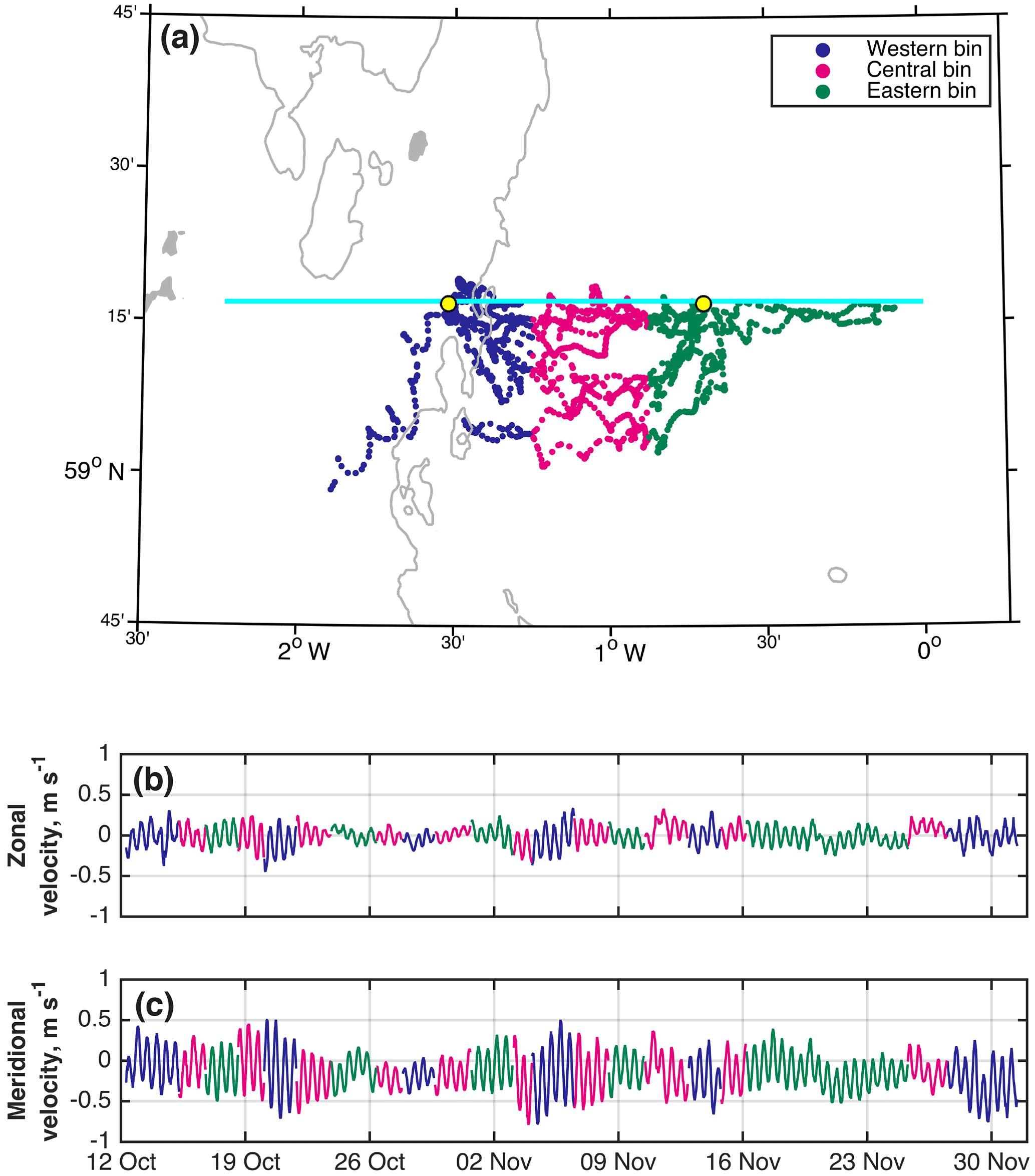
Figure 2 (a) The location of glider dives along the JONSIS section (cyan line), with dives coloured by longitudinal bin (see legend in a). The location of the current meters is shown by the yellow dots. The 100 m isobath is shown in grey. (b) Zonal and (c) meridional DAC velocities coloured by bin (same colour scheme as a).

2 Glider-derived tidal velocities

2.1 Method

Between 12 October and 1 December 2013, the glider (Eriksen et al., 2001) completed 10 partial occupations of the Joint North Sea Information System (JONSIS) hydrographic section (Turrell et al., 1996). Occupations took between 3 and 11 days, depending on how much of the section was sampled. The 127 km long section between 2.23^∘ W and the prime meridian at 59.28^∘ N (Fig. 1) crosses the combined path of the two western Atlantic inflows into the north-western North Sea: the FIC and the East Shetland Atlantic Inflow (Turrell et al., 1996). Bathymetry along the section varies between 69 and 143 m, deepening eastward. All bathymetric data used in this study were extracted from the GEBCO dataset (GEBCO_08 grid, version 20100927, http://www.gebco.net; resolution 30 arcsec). While it is possible to estimate bathymetry from the glider's altimeter observations, we believe that bathymetry from a databank for a well-studied region such as the North Sea is likely more accurate. Glider dives were, on average, 20 min and 300 m apart; as one dive comprises two profiles, profiles are therefore an average of 150 m apart. Most dives sampled the full water column. DAC observations are obtained incidentally during a glider's flight as the glider is advected by the flow over the duration of a dive–climb cycle. On surfacing, the glider compares its actual GPS-determined position with its position as estimated by dead reckoning; the difference is attributed to advection by the DAC (Eriksen et al., 2001; Merckelbach et al., 2008). The accuracy of DAC observations was improved post-deployment by optimising the hydrodynamic model of the glider's flight (Frajka-Williams et al., 2011). DAC observations were visually inspected to ensure that there were no systematic errors due to the glider's compass calibration, and the method described in this section was repeated using DAC observations from only eastbound and westbound occupations. No systematic difference between results obtained from the two samples was found, indicating that the observations are not affected by compass error.

DAC velocities were divided into three longitudinal bins along the JONSIS section (Fig. 2a), the boundaries being chosen such that each bin contained an approximately equal number of dives: 502 in the eastern bin, 514 in the central bin, and 503 in the western bin. Binned velocities were treated as three discontinuous time series (Fig. 2b and c). At the central longitude of each bin, the amplitude and phase of the M² and S² tidal constituents were determined using harmonic analysis (Thomson and Emery, 2014). These results were used to construct tidal ellipses along the JONSIS section (Fig. 3). Combined M² and S² (hereafter denoted M² + S²) zonal and meridional velocities were then calculated at the time of each glider dive. Finally, tidal velocity was linearly interpolated onto that dive's longitude to construct a time series of tidal velocity along the glider's overground track – that is, a time series of tidal velocities with data points at the time and location of each dive (Fig. 2a). These are hereafter referred to as along-track velocities (Fig. 4). Nearest-neighbour extrapolation was used for dives to the east and west of the three bins; extrapolation is necessary because some dives lie to the east and west of the central points of the eastern and western bins respectively.

The accuracy of the glider-derived ellipses and consequently of the derived tidal currents is dependent on the number of dives that fall within a bin, and the number of bins determines the number of points along the section at which the tide may be resolved. There is therefore a trade-off between the number of constituents that can be resolved in the harmonic analysis and the spatial resolution. For a regularly spaced continuous time series, the Rayleigh criterion (Δf = 1∕T, where Δf is the difference in frequency between two constituents, and T is the length of the time series) dictates the minimum length of time series needed to separately resolve constituents of different frequencies. To resolve the M² and S² constituents from a combined signal, a time series of at least 14.8 days is needed: that is, the cycle introduced into tidal signals by the interaction of the M² and S² constituents, known as the spring–neap cycle. The Rayleigh criterion is harder to apply to a time series of irregularly spaced DAC, particularly when temporal discontinuities are introduced by the binning process (Fig. 2). Instead, setting the limits of each bin such that an equal number of dives falls in each ensures that amplitude and phase estimates are of a comparable accuracy across the section. The cumulative length of time that the glider spends in each bin is 14.6, 17.1, and 17.7 days for the western, central, and eastern bin respectively, which is approximately equal to or greater than the minimum length of time needed to separately resolve the M² and S² constituents in a regularly spaced continuous time series. Separating the time series into four or more bins necessarily reduces the number of dives and the length of time the glider spends in each bin. Using four or more bins resulted in S² ellipses with unrealistic amplitudes and inclinations, suggesting an inadequate resolution of this weaker constituent.

Two current meters were deployed on the JONSIS section for a period covering the glider deployment: an Aanderaa Seaguard single-point current meter at a depth of 40 m (1.52^∘ W; Fig. 2a) and a Nortek AWAC profiling current meter that took measurements in 4 m bins centred from 9 to 89 m below the surface (0.70^∘ W; Fig. 2a). Observations from the profiling current meter were depth-averaged for comparison with glider DAC. The amplitude and phase of the M² and S² tidal constituents were determined from the current meter records using the same harmonic analysis as for the glider data. To compare the results of our method with an established alternative, estimates of M² and S² amplitude, phase, and velocity were extracted from the TPXO inverse model European shelf solution (Egbert and Erofeeva, 2002; Egbert et al., 1994, 2010) using the Tidal Model Driver software for MATLAB (available at http://esr.org/research/polar-tide-models/tmd-software).

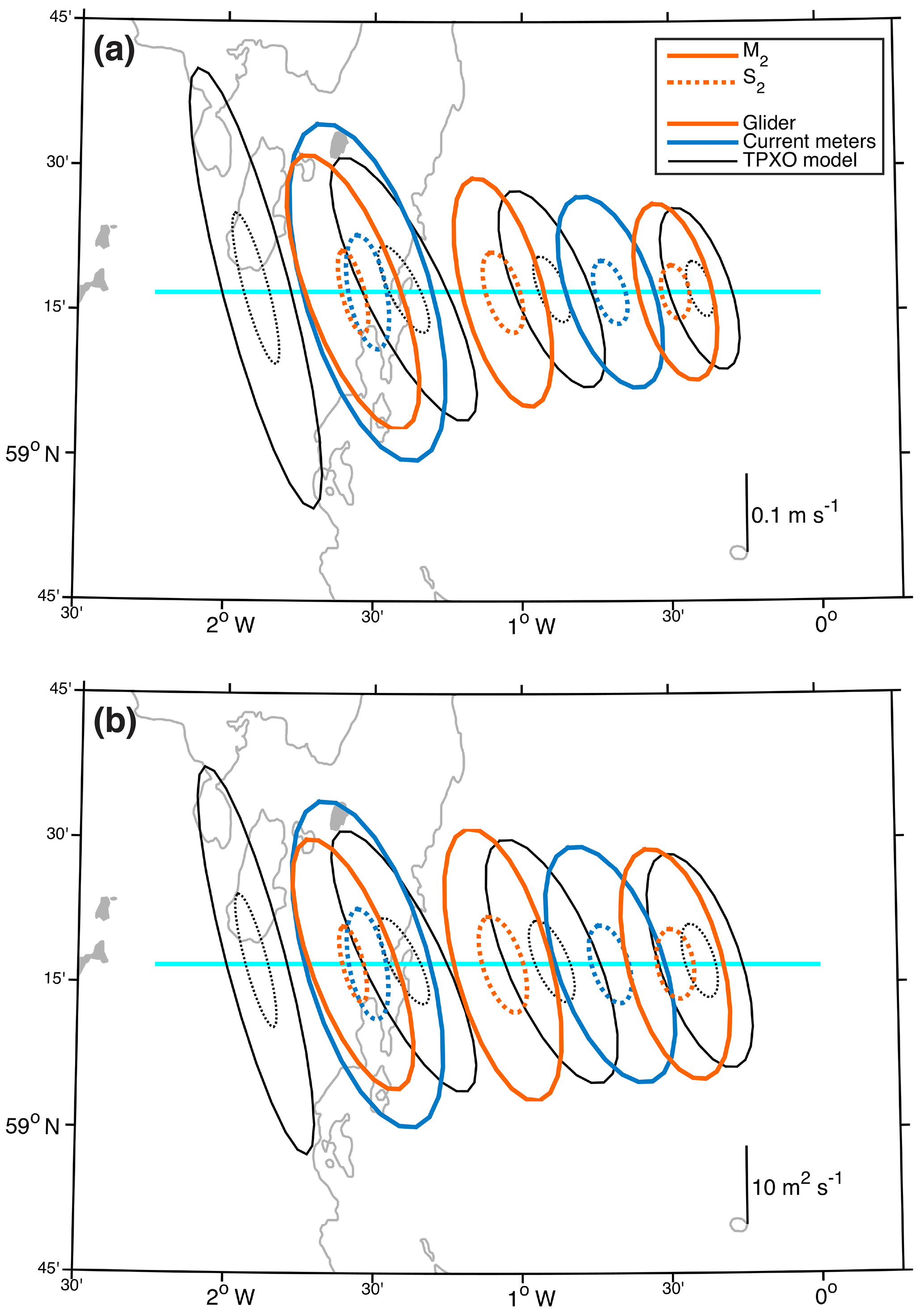
Figure 3 (a) Tidal ellipses from glider observations (orange), current meter observations (blue), and the TPXO tide model (every fifth grid point, black). (b) Tidal transport ellipses, with colours as in panel a. In both panels, solid lines are for the M² constituent; dotted lines are for the S² constituent. The JONSIS section is shown in cyan and the 100 m isobath is shown in grey. Note that the scale of the ellipses is different in each panel.

2.2 Tidal ellipses

Tidal ellipses of the glider-derived tide show a decrease in the amplitude of zonal and meridional tidal velocity with distance offshore (Fig. 3a). Semi-major axes are consistently larger than semi-minor axes, and the offshore decrease in the magnitude of the semi-major axes is greater than the offshore decrease in semi-minor axes. The smaller rate of change in the eastern part of the section is because bathymetry gradients are smaller than in the west. Velocity amplitudes were multiplied by the mean water depth in each bin to derive ellipses of tidal transport per unit width (Fig. 3b). Compared with velocity amplitude, transport amplitude changes less markedly with distance offshore, suggesting that the greater tidal velocities observed in shallow water than in deep water are primarily a result of volume continuity rather than the exponential offshore decay of the tidal Kelvin wave.

Glider velocity ellipses compare well with velocity ellipses from the current meter observations and the TPXO model (Fig. 3a). Ellipses from the three sources indicate clockwise rotation of the tide. The ellipse from the western, single-point current meter observations (Figs. 2a and 3) is likely larger (i.e. indicating faster tidal velocities) than the depth-mean glider and TPXO ellipses because tidal currents at the depth of this current meter (40 m) are less influenced by bottom friction than are depth-average velocities. Comparing glider ellipses with the TPXO ellipses at the same location, the difference between the M² semi-major axes is 0.10 m s⁻¹ (25 %) in the western bin and 0.01 m s⁻¹ in the central and eastern bins (2 and 4 % respectively). The difference between the M₂ semi-minor axes is 0.01 m s⁻¹ in all three bins (< 1, 8, and 15 % in the western, central, and eastern bins respectively). The phases of the M² ellipses differ by 10, 7, and 11^∘ in the western, central, and eastern bins respectively. S² semi-major axes differ by 0.05 m s⁻¹ (44 %) in the western bin and by 0.01 m s⁻¹ in the central and eastern bins (8 and 9 % respectively). S² semi-minor axes differ by 0.01 m s⁻¹ in all three bins (48, 18, and 19 % in the western, central, and eastern bins respectively). The phases of the S² ellipses differ by 7, 2, and 17^∘ in the western, central, and eastern bins respectively. Percentage differences between the S² ellipses are larger in the western bin because the magnitude of the glider-derived S² tide is smaller than in the central and eastern bin. Differences between the ellipses in the western bin could be greater than in the central and eastern bins because the TPXO model is an inversion of satellite altimeter observations, which are less reliable near coastlines (Egbert and Erofeeva, 2002). The glider ellipses are potentially a more accurate characterisation of the tide in this part of the section.

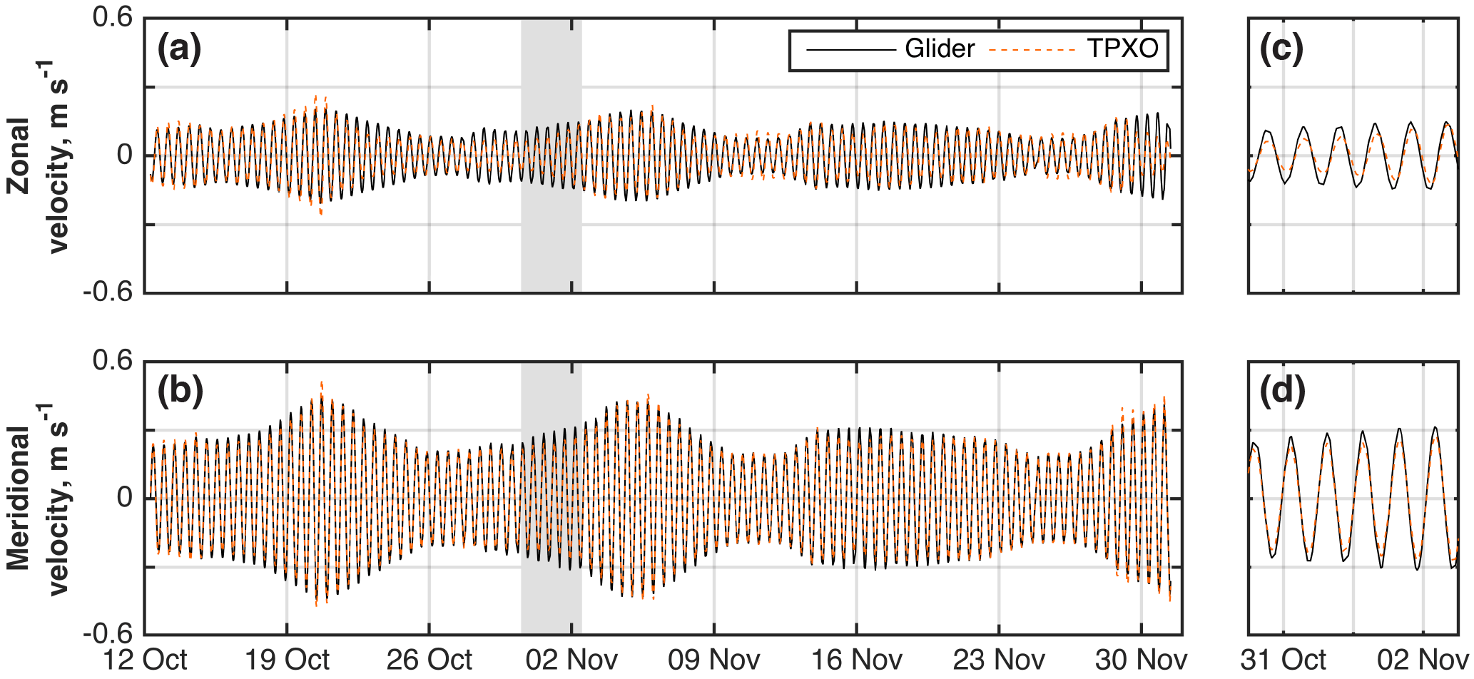
Figure 4 (a) Zonal and (b) meridional velocity. Panels (c) and (d) are zoomed-in excerpts of (a) and (c) respectively. The region shown in (c) and (d) is marked by the grey box in panels (a) and (b) respectively. In all panels, the solid black line is the M² + S² tidal velocity determined from the glider observations and the dashed orange line is the M² + S² tidal velocity from the subsampled TPXO model.

2.3 Glider-derived tidal velocities

To quantify the accuracy of the glider-derived tide (Fig. 4), the along-track M² + S² velocity time series are compared with the M² + S² along-track time series from the TPXO model sampled at full resolution. Unlike the current meter observations, this model provides estimates of tidal velocity across the entire JONSIS section. The root mean square differences (RMSDs) between the glider- and the TPXO-derived tides are 0.03 and 0.02 m s⁻¹ for the zonal and meridional velocities respectively.

To determine the extent to which the difference between the glider- and TPXO-derived time series may be attributed to the comparatively low resolution of the glider-derived tide, we firstly compare the fully sampled TPXO tide with the TPXO tide sampled at the same locations as the glider-derived tide (i.e. the centre of each of the three bins; Fig. 2). Velocity time series are extracted from the TPXO model at the central point of each glider bin and at the time of each glider dive. These velocities are interpolated zonally onto the location of each dive, replicating the method used to calculate the glider-derived tide. The RMSDs between the fully sampled and subsampled TPXO time series are 0.04 and 0.02 m s⁻¹ for the zonal and meridional velocities respectively. Secondly, to simulate a longer glider deployment with more dives from which it would be possible to use smaller spatial bins and so increase spatial resolution, we compare the fully sampled TPXO tide with the TPXO model subsampled every 0.5^∘ longitude between 2.5^∘ W and the prime meridian. This decreases the zonal RMSD to 0.03 m s⁻¹; the meridional RMSD remains 0.02 m s⁻¹. The spatial resolution of the glider-derived tide appears to have little influence on the results compared with the output of a high-resolution tide model.

The ability to use glider DAC to estimate along-track tidal velocity to within ±0.02 to 0.04 m s⁻¹, even when the tide may be resolved at only a few points along a section, could be of considerable use in regions where tide models are unreliable or unavailable, thereby enhancing the utility of gliders, for example in remote regions such as the Antarctic shelf. In order to use this method on DAC observations from other glider missions, we make the following recommendations:

1. obtain repeat occupations of the same transect;

2. set the transect length so as to avoid aliasing the spring–neap cycle – i.e. avoid individual occupations lasting around 1 or 2 weeks;

3. optimise the hydrodynamic model of the glider's flight (Frajka-Williams et al., 2011) to obtain accurate DAC observations; and

4. do not attempt to resolve more constituents than may be accurately resolved given the length of each binned discontinuous time series.

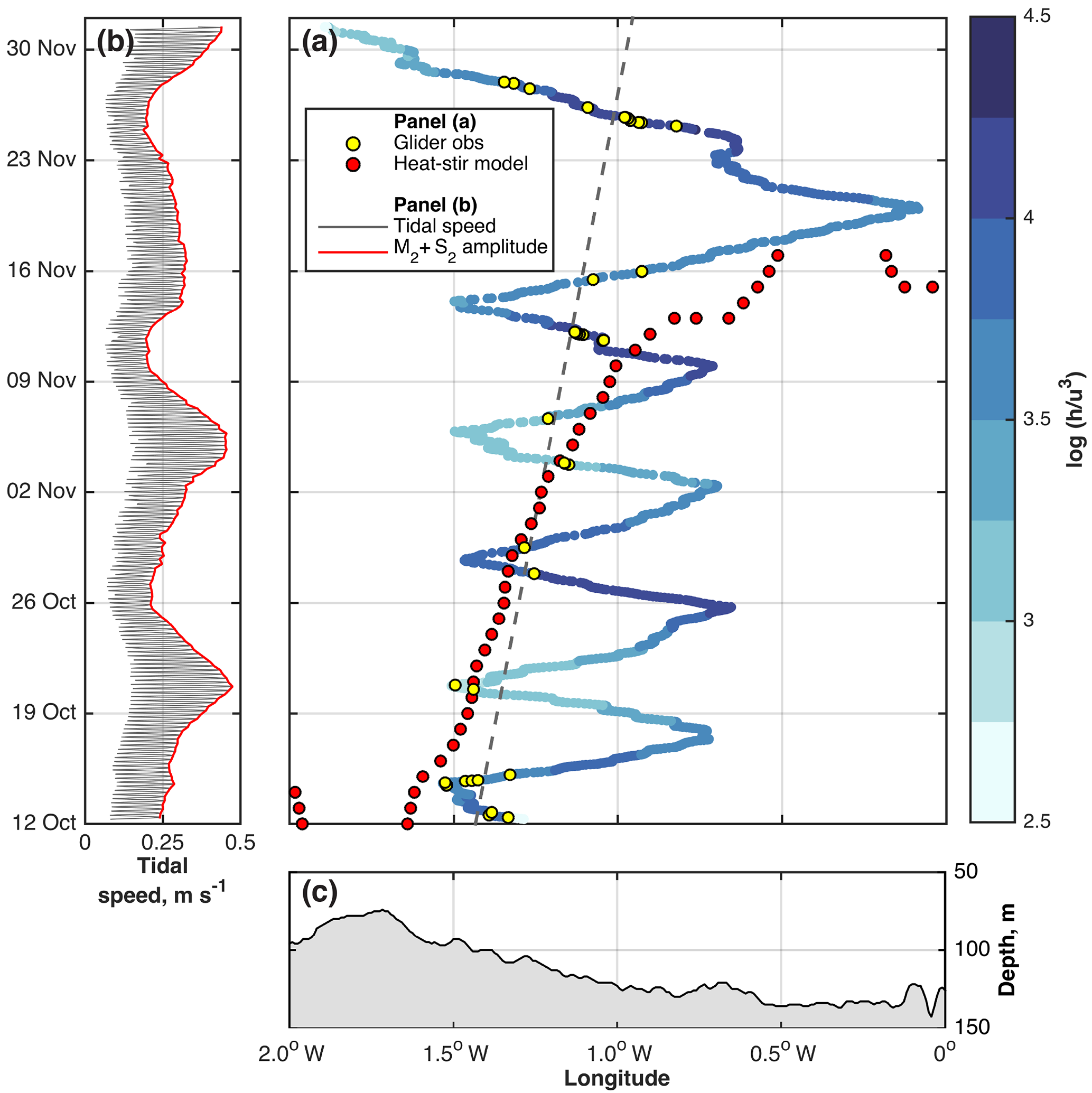
Figure 5 (a) Hovmöller plot of log(h∕u³) (colour scale) from glider observations. Yellow circles mark the observed locations of the front. The dashed grey line is the line of best fit through these points. Red circles mark the location of the front as modelled by the heating–stirring model. (b) M² + S² tidal speed (m s⁻¹; grey line) at the location of each glider dive as calculated using the glider-derived tidal velocities. The red line joins up the maximum speeds and is the estimate of tidal velocity amplitude, u, used to calculate log(h∕u³) in (a). (c) Bathymetry (m) along the JONSIS section – i.e. h in log(h∕u³).

3 Frontal location

We apply the glider-derived tide described in the previous section to study the location of a front in the north-western North Sea. Specifically, we investigate the extent to which the location of the front may be explained by heating–stirring interactions, a principal component of which is tidal speed. Furthermore, this analysis serves as an illustration of a potential application of the method. We use TEOS-10 variables (IOC, SCOR, and IAPSO, 2010) in this analysis.

The location of the front as determined from the glider observations is shown in Fig. 5. The front is defined to be where the top–bottom temperature difference is 0.5 ^∘C. This definition has the advantage of being straightforward to calculate, both from observations and models, and follows the approach used in previous studies (Bowers and Simpson, 1987; Holt and Umlauf, 2008; O'Dea et al., 2012). On a number of crossings of the front, the top–bottom temperature difference equals 0.5 ^∘C at several points (Fig. 5a). This is because the front often covers a zonal distance wider than that between glider dives. Observations of frontal location are not corrected for zonal tidal advection of the front. Instead, we acknowledge a zonal uncertainty in frontal position of ±2 km (0.04^∘ longitude), which is the mean zonal tidal displacement during the deployment.

We calculate log(h∕u³) at the time and location of each glider dive. The amplitude of tidal speed used to calculate log(h∕u³), in place of the amplitude of the M² tidal speed, is that of the M² + S² constituents; this is to capture changes in tidal speed over the spring–neap cycle. The M² + S² amplitude is derived from the along-track glider-derived tide: we extract a time series of the maximum speed achieved over each tidal cycle (Fig. 5b, red line) and interpolate this onto the time of each glider dive.

Values of log(h∕u³) at the front vary considerably over time (Fig. 5a), from below 3 around 21 October to over 4 around 12 November. Some of this range may likely be attributed to the width of the front, which can cover a range of values of log(h∕u³) at this high spatial and temporal resolution (Hughes, 2014). Often, the frontal value of log(h∕u³) lies outside the range 2.7 ± 0.4 typically used as the critical value for the north-western European shelf region (Simpson and Sharples, 1994). However, our modified definition of the amplitude of tidal speed (i.e. M² + S²) precludes a direct comparison of our values of log(h∕u³) with those previously published. Using only the M² tidal speed allows for comparison with previous studies, although this results in a log(h∕u³) distribution that changes only spatially and that does not account for changes in the amplitude of tidal speed over the spring–neap cycle. Values of log(h∕u³) at the front when only the M² constituent is included (not shown) fall between 3.25 and 3.75. These M²-only values cover a narrower range than when the S² constituent is included and all fall outside the range 2.7 ± 0.4.

Pingree and Griffiths (1978) note that fronts in the vicinity of the Orkney and Shetland archipelagoes are found at higher than expected values of log(h∕u³), although they modify the theory to account for bottom drag, so their values of the critical contour are not directly comparable. Salinity gradients and geographical variations in the surface heat flux are suggested as possible reasons for the deviation from predictions. Hughes (2014), using a heat flux appropriate to the north-western North Sea, concluded from a modelling study that the critical value for frontal location in the region should be 3.4; the applicability of this value was confirmed by examination of 28 years (1982–2008 inclusive) of satellite observations of sea-surface temperature (Hughes, 2014). The higher critical value is attributed to the reduced heat flux and enhanced wind mixing at the latitudes of the north-western North Sea compared with the latitudes of the Celtic Sea (Hughes, 2014), which is the site of much previous work on the h∕u³ criterion (Simpson and Hunter, 1974). The 3.4 value falls within the range of values reported in this study; our observations enable assessment of the critical value derived by Hughes (2014) against full-depth observations of the front.

We acknowledge that the accuracy of log(h∕u³) as a predictor of frontal location is greater in summer when surface heating is the dominant control on frontal location than it is at other times of year. However, in the absence of full-depth glider observations of the front in summer, the higher frontal values reported here appear to confirm the tendency, found in both model results and surface observations, for the front in the north-western North Sea to be found at higher critical values of log(h∕u³) than those once thought applicable to the entire north-western European continental shelf (Simpson and Sharples, 1994). Glider observations of the front in summer are desirable.

There does not appear to be adjustment of frontal location with the spring–neap cycle, although the effects of such adjustment would be much greater immediately after frontal development, i.e. in late spring and early summer (Simpson and Bowers, 1981). Furthermore, some of the additional mixing energy available at spring tides is expended reducing stored potential energy on the stratified side of the front rather than moving the front itself, limiting the extent of spring–neap frontal adjustment (Simpson and Bowers, 1981). Instead, the dominant signal in frontal location is its offshore movement over the course of the glider deployment (Fig. 5a). From a longitude of approximately 1.4^∘ W at the start of the deployment, the front moves eastwards into deeper water, reaching approximately 1^∘ W by the middle of November. It then widens considerably towards the end of the deployment, being spread between 1.4 and 0.8^∘ W at the time of the final occupation (19 November–1 December). A least-squares line of best fit through the frontal locations indicates that the front moves eastward at a rate of 0.53 ± 0.06 km day⁻¹.

3.1 Comparison with model output

We compare the observations of frontal location with the output of a numerical model of heating–stirring processes to identify if and when heating–stirring interactions control frontal location during the deployment. We use the open-source, one-dimensional heating–stirring model of Simpson and Bowers (1984). The model is straightforward to run; it may be readily adapted to suit the study region and to work with the glider-derived tide described in Sect. 2; it includes only the physical heating–stirring processes used to describe frontal location by Simpson and Hunter (1974) and Simpson and Bowers (1984), as also described in Sect. 1. Consequently, the model allows us to investigate the extent to which heating–stirring interactions influence the location of the observed front (Fig. 5).

The model is forced with meteorological parameters from the NOCS Flux v2.0 dataset (Berry and Kent, 2009, 2011; National Oceanography Centre, 2008) and with tidal speed. It simulates a temperature profile for a water column of a given depth. Approximately 55 % of incoming heat energy is absorbed at the surface, the remaining 45 % being distributed exponentially with depth. This distribution is typical for coastal waters (Ivanoff, 1977). Once heat loss to the atmosphere has been extracted from the surface layer, the additional heat is mixed downwards until the increase in potential energy equals the effective stirring energy input from the wind over the given time step; the profile is then further modified by bottom-up tidal mixing until the increase in potential energy equals the effective stirring energy input from the tide. If the net surface heat flux is negative (i.e. heat loss) the model simulates convection. The new surface temperature is then used to calculate the surface heat flux for the subsequent time step (Simpson and Bowers, 1984). The original model is modified to include the improved parameterisation of heat exchange through the sea surface implemented by Sharples et al. (2006) and Hughes (2014) and to include the additional energy available for bottom-up mixing provided by a constant background flow of 0.1 m s⁻¹ following the method of Hughes (2014). The magnitude of the background flow is chosen to be representative of the values observed in the region (Turrell, 1992; Turrell et al., 1990, 1996). The stirring effects of a persistent background flow were not included in the original formulation of the h∕u³ theory, but the presence of Atlantic inflow in the study region makes it a necessary addition.

Temperature profiles are simulated at every 0.1^∘ longitude along the JONSIS section and for every day of the glider deployment at daily resolution. The diurnal heating–cooling cycle is not resolved. We take as the tidal speed the meridional M² + S² velocity amplitude midway between spring and neap tides and use the glider-derived tide to capture the offshore decay in tidal amplitude. Meridional M² + S² velocity amplitude is calculated at the centre of each bin (Fig. 2a) and is interpolated onto the longitude of each model grid point. We do not simulate the spring–neap cycle because spring–neap frontal adjustment is not observed in the glider sections (Fig. 5a).

Using the same definition of frontal location as used for the glider profiles, the heating–stirring model places the front in a similar position to the observations during the first 4 weeks of the deployment (Fig. 5a), albeit approximately 0.1^∘ further west prior to 15 October. The coastal front that appears in the far west of the section between 12 and 14 October is not considered here because it is outside the longitudinal range of the glider sections. We test the sensitivity of the results to the speed of the background flow. Modifying the background flow speed by ±0.03 m s⁻¹, a reasonable range, makes no difference to the results at the bottom of the range and shifts the front by approximately 0.05^∘ longitude (3 km) eastward at the top of the range.

The similarity between the heating–stirring model (with a realistic background current of 0.1 m s⁻¹ and an intermediate tidal amplitude) and the observations during the first 4 weeks of the glider deployment suggests that the interaction between surface heat fluxes and tidal mixing explains the location of the front during this period. Specifically, the negative surface heat flux (i.e. heat loss to the atmosphere) during the period of the glider deployment (Fig. 6) means that stratification is maintained only by heat remaining in the water column after the period of summer heating (April to September; Fig. 6). As heat is progressively lost to the atmosphere, the influence of tidal stirring becomes ever more dominant, pushing the front into deeper water (Fig. 5). However, the persistence of the observed front after 17 November 2013 and its slower easterly advance compared with that of the modelled front (1.59 ± 0.08 km day⁻¹; rate excludes the secondary front that emerges on 15 November 2013 around 0.1^∘ W) suggests that the heating–stirring balance is not the primary control on frontal location in the latter period of the glider deployment (i.e. after approximately 4 November).

3.2 Comparison with observations

The existence of the front in the observations despite its disappearance in the heating–stirring model suggests that processes other than heating–stirring interactions are responsible for maintaining the front into the latter weeks of the glider deployment. In addition to the horizontal temperature gradient observed by the glider on its final two crossings of the front (observations from the penultimate crossing are shown in Fig. 7) a horizontal salinity gradient exists between the relatively fresh waters in the west of the section and the relatively saline waters in the east. Salinity is a useful water mass tracer in the region and permits identification of the water masses present in the observations. The salinity minimum (< 35.25 g kg⁻¹) to the west of the section is indicative of coastal water from around Scotland, which is freshened by river input and run-off (Dooley, 1974; Turrell et al., 1992); the salinity maximum (> 35.25 g kg⁻¹) to the east of the section is indicative of water of recent Atlantic origin (Turrell et al., 1992). Intermediate salinity (∼ 35.275 g kg⁻¹) and minimum temperature (< 7.5 ^∘C) is indicative of water that has spent the previous summer isolated beneath the seasonal thermocline (Hill et al., 2008; Svendsen et al., 1991; Turrell et al., 1992); this has been called Cooled Atlantic Water (Turrell et al., 1992). The southward penetration of Atlantic water from the open northern boundary of the North Sea elevates the salinity of CAW (Hill et al., 2008). The heating–stirring model cannot reproduce these water masses: they are not formed locally by heating–stirring interactions and their distribution in the northern North Sea is controlled by advection. The temperature distribution created by these water masses is such that a horizontal temperature gradient is maintained. In particular, the bottom front, which is the most dynamically significant feature of the frontal system (Hill et al., 2008; Sheehan et al., 2017), is maintained by the presence of the Atlantic-influenced CAW.

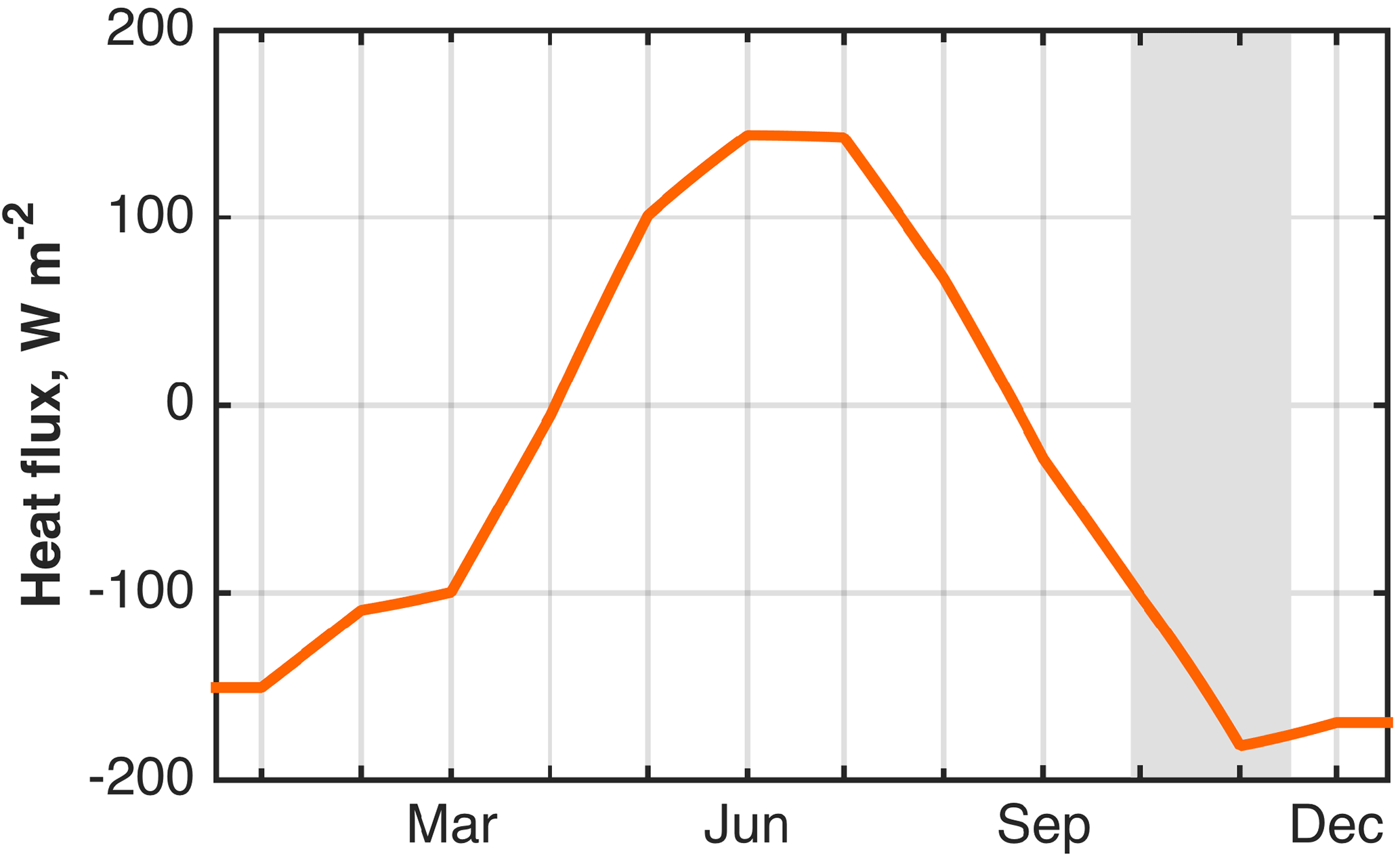
Figure 6 Total surface heat flux (i.e. the sum of latent, sensible, incoming radiative, and outgoing radiative fluxes; W m⁻²) in 2013 averaged zonally across the JONSIS section. Positive fluxes indicate energy transfer into the ocean. Latent, sensible, and outgoing radiative fluxes are calculated by the heating–stirring model using the method of Sharples et al. (2006) from monthly mean meteorological parameters extracted from the NOCS Flux v2.0 dataset (National Oceanography Centre, 2008). Monthly mean incoming radiative flux is extracted from NOCS Flux v2.0. The period of the glider deployment is indicated by the grey box.

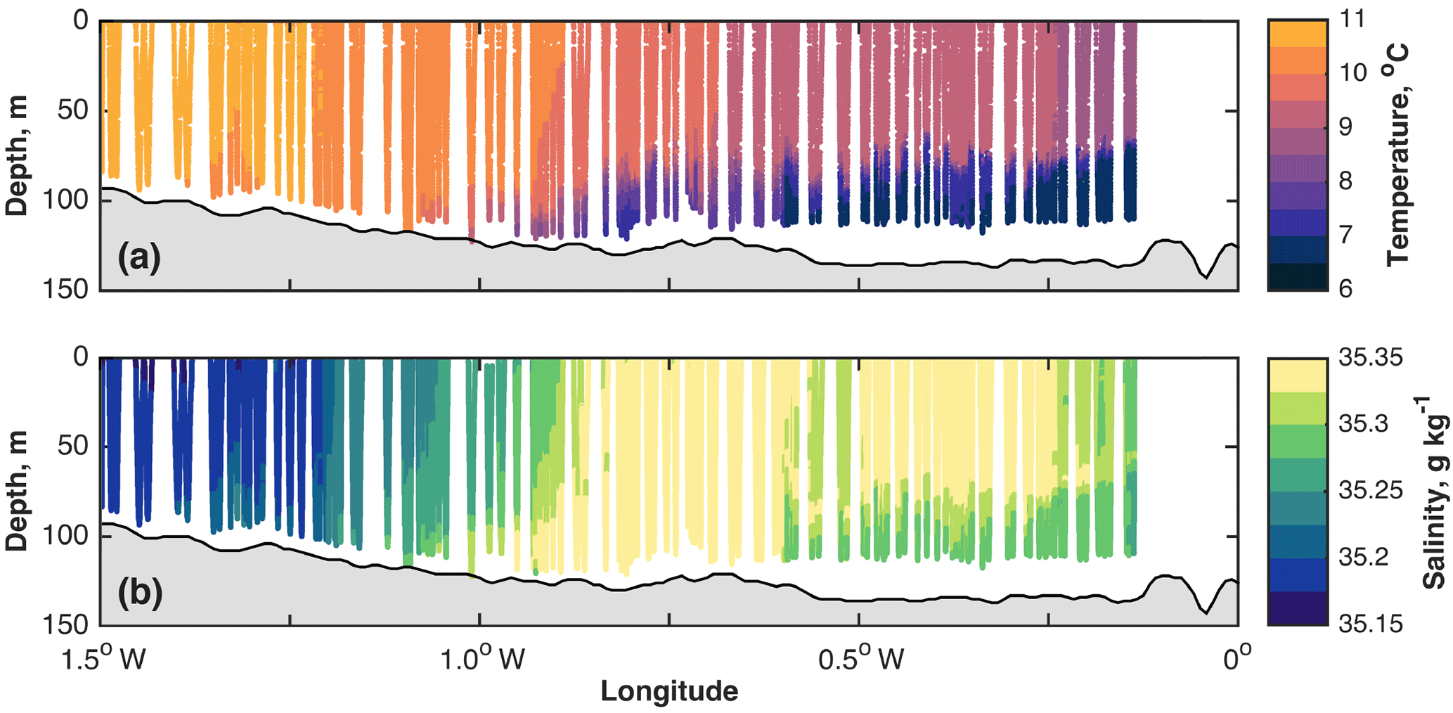
Figure 7 (a) Conservative temperature (^∘C) and (b) absolute salinity (g kg⁻¹) from the penultimate glider occupation of the JONSIS section (14–20 November 2013).

The glider observations presented in Figs. 5 and 7 demonstrate that a front can exist in the north-western North Sea independently of heating–stirring interactions. Such a front is clearly not simply a tidal mixing front. However, during the first part of the deployment, the observed frontal location compares well to frontal location as predicted from consideration of only heating–stirring interactions. We propose that the observed front is a hybrid between a tidal mixing front and a front which forms due to horizontal gradients between adjacent water masses in a region of complex water mass interaction. In winter, in the absence of local solar heating and when temperature variation between water masses is negligible, there is a salinity front in the region that gives rise to thermohaline flow (Sheehan et al., 2017). In summer, we propose that local heating–stirring interactions modify the water masses to the extent that the front is moved to a position as predicted by consideration of heating–stirring interactions. The present study does not include observations of the front at this time, but when forced with an annual cycle of multi-decadal mean meteorological values, the heating–stirring model places a tidal mixing front at approximately 1.5^∘ W in summer; the front is found at the same location in multi-decadal summertime averages of JONSIS section hydrography (Sheehan et al., 2017). The observations presented in this study (Fig. 5a) capture the period in the annual cycle when, in 2013, the front makes the transition from being a front controlled by heating–stirring interactions to being a front controlled by the distribution of water masses.

4 Summary

We have demonstrated that glider DAC observations may be used to determine tidal velocities at the time and location of each glider dive to within ±0.04 m s⁻¹. Glider-derived tidal velocities compare favourably to output from current meters and the TPXO tide model. The method enhances the utility of gliders as an ocean-observing platform, particularly in regions such as Antarctica where tide models are known to be poorly constrained. The method could also be extended to two dimensions: for instance, to two gliders flown along parallel transects or to one or more gliders flown in a butterfly pattern. A longer deployment than the 2-month deployment presented in this study would allow for more tidal constituents to be resolved from the resulting DAC time series.

Glider-derived tidal velocities were applied to study the location of a front in the north-western North Sea. The results of a one-dimensional heating–stirring model and comparison of these results with the glider's hydrographic observations demonstrated that salinity gradients and the distribution of water masses are important controls on frontal location in the region, in addition to surface heating and primarily tidally induced mixing. A water mass distribution exists which gives rise to a frontal boundary in temperature and salinity. In the absence of significant surface heating, this is the primary source of a frontal boundary and therefore the primary control on frontal location. In summer, heating–stirring interactions modify the water masses, enhancing the background temperature gradient such that heating–stirring interactions become the primary control on frontal location. This situation persists until the autumn: the observations presented in this study capture the period during which, in 2013, the front transitions from being primarily a tidal mixing front to being primarily a front between different water masses. The inter-annual variability of the timing of this transition is a topic for further investigation.

Water mass distribution and the attendant spatial gradients of thermal and haline buoyancy are likely to be important in shelf seas where significant incursions of oceanic water are found, such as the north-western North Sea, the South China Sea (Shaw, 1991; Su, 2004), along the eastern coast of the United States (Blanton et al., 1981) and around Antarctica (Moffat et al., 2009). While heating–stirring interactions are ubiquitous in shelf seas, fronts in such regions may persist during periods when local heating–stirring interactions would not promote frontal formation. Consequently, controls on frontal location may change over an annual cycle. Given the thermohaline flows commonly associated with shelf sea fronts and the influence that fronts have on the distribution of physical and biogeochemical properties (Hill et al., 2008; Turrell, 1992), this has important implications for the dynamics, ecology, and management of shelf sea regions.