the Creative Commons Attribution 4.0 License.
the Creative Commons Attribution 4.0 License.
 | 29 Oct 2018
Structure and dynamics of mesoscale eddies over the Laptev Sea continental slope in the Arctic Ocean
Igor V. Polyakov
Laurie Padman
An T. Nguyen
Heat fluxes steered by mesoscale eddies may be a significant, but still not quantified, source of heat to the surface mixed layer and sea ice cover in the Arctic Ocean, as well as a source of nutrients for enhancing seasonal productivity in the near-surface layers. Here we use 4 years (2007–2011) of velocity and hydrography records from a moored profiler over the Laptev Sea slope and 15 months (2008–2009) of acoustic Doppler current profiler data from a nearby mooring to investigate the structure and dynamics of eddies at the continental margin of the eastern Eurasian Basin. Typical eddy scales are radii of the order of 10 km, heights of 600 m, and maximum velocities of ∼0.1 m s−1. Eddies are approximately equally divided between cyclonic and anticyclonic polarizations, contrary to prior observations from the deep basins and along the Lomonosov Ridge. Eddies are present in the mooring records about 20 %–25 % of the time, taking about 1 week to pass through the mooring at an average frequency of about one eddy per month.
We found that the eddies observed are formed in two distinct regions – near Fram Strait, where the western branch of Atlantic Water (AW) enters the Arctic Ocean, and near Severnaya Zemlya, where the Fram Strait and Barents Sea branches of the AW inflow merge. These eddies, embedded in the Arctic Circumpolar Boundary Current, carry anomalous water properties along the eastern Arctic continental slope. The enhanced diapycnal mixing that we found within EB eddies suggests a potentially important role for eddies in the vertical redistribution of heat in the Arctic Ocean interior.
- Article
(15500 KB) - Full-text XML
-
Supplement
(847 KB) - BibTeX
- EndNote


The decline in Arctic sea ice area and volume is one of the most prominent features of global climate change. The observed sea ice decline over the last 2 decades is consistent with an average ocean heat flux surplus of just ∼1 W m−2 (Kwok and Untersteiner, 2011). Thus, relatively small changes in the flux of heat from the intermediate warm ocean layers to the fresh and cold waters of the surface mixed layer (SML) and sea ice might therefore contribute to the ice loss.

Figure 1(a) Map showing the location of the M1f mooring (yellow circle) over the continental slope of the Laptev Sea in the Eurasian Basin of the Arctic Ocean in 2007–2011. The position of the M1g mooring is not distinguishable from M1f at these scales. Greenland (GR), Spitsbergen (SP), Franz Josef Land (FJL), St. Anna Trough (SAT), Severnaya Zemlya (SZ), and Novosibirskiye Islands (NO) are indicated. Red arrows show a schematic pattern of Atlantic Water (AW) circulation in the Eurasian Basin. Bottom depth in meters is shown by color. (b) Schematics of moorings deployed at the Laptev Sea slope in 2007–2011 (M1f mooring) and in 2008–2011 (M1g mooring). (c) Mean temperature (red) and salinity (blue) profiles in the Eurasian Basin, averaged for winter months (DJF), taken from a polar hydrographic climatology dataset (Steele et al., 2001). Horizontal green lines show the limits of the surface mixed (SML), cold halocline (CHL), and AW layers.
However, a strongly stratified cold halocline layer (CHL) may effectively suppress heat fluxes from the relatively warm Atlantic Water (AW) located between ∼150 and 800 m depths (Fig. 1c; e.g., Aagaard et al., 1981; Rudels et al., 1996). Therefore, there is a need to determine if mechanisms exist to transport heat from the warmer AW layer to the surface and, if so, how those processes might change in future Arctic states.
Mesoscale eddies are an important component in Arctic Ocean dynamics and may comprise the major portion of total kinetic energy attributed to oceanic mesoscale processes in the Arctic Ocean (e.g., Hunkins, 1974; Manley and Hunkins, 1985; Woodgate et al., 2001; Dmitrenko et al., 2008; Timmermans et al., 2008; Zhao et al., 2016). Impacting the ocean interior through diapycnal mixing and lateral transport, these eddies may also contribute significantly to the oceanic transport of heat, nutrients, pollutants, and other tracers within polar regions (e.g., Smith, 1984; Manley, 1987; Lankhorst, 2006; Kadko et al., 2008; Nudds and Shore, 2011; Crews et al., 2018).
The first observations regarding mesoscale eddies in the eastern Arctic Ocean were carried out in Fram Strait (a ∼500 km wide strait between Spitsbergen and Greenland) by a submarine transect over the East Greenland polar front, where several warm-core “patches” with horizontal sizes up to ∼ 25 km in diameter were found (Wadhams et al., 1979). A series of “small” cyclonic eddies with rotational velocities in the range of 5–20 cm s−1 were also found within the mixed layer and the upper halocline during the Norwegian Remote Sensing Experiment northwest of Spitsbergen in 1979 (Johannessen et al., 1983, 1987).
The horizontal size of the reported Eurasian Basin (EB) eddies was very close to estimates of ∼20 km in diameter for Canada Basin eddies (Manley and Hunkins, 1985); vertical extents, however, were much larger. For example, Woodgate et al. (2001) found isolated rotating current events, attributed to passing eddies, within a water column of up to ∼1600 m of depth at the Lomonosov Ridge. Approximately the same vertical eddy size (∼1700 m) was found by Aagaard et al. (2008) in the central Arctic Ocean. Dmitrenko et al. (2008) reported vertical eddy extensions as large as ∼800 m in the eastern EB. These observations suggest a deep source for these eddies, similar to the source reported for the Beaufort Gyre eddies by Carpenter and Timmermans (2012), but fundamentally different from the more commonly observed halocline eddies in the Canada Basin.
In this paper, we document properties of mesoscale eddies along the continental slope of the Laptev Sea in the EB of the Arctic Ocean using recent temperature, salinity, and velocity observations from moorings. We first describe datasets and basic analysis methods (Sect. 2). We then document the statistical properties of EB mesoscale eddies based on 4 years of mooring observations over the Laptev Sea slope (Sect. 3). Section 4 describes the identification of eddy origins for eddies observed by the moorings, and in Sect. 5 we estimate the effect of eddies on vertical mixing. We conclude with a discussion and summary of results in Sect. 6.
2.1 Observational data
Observations were collected using a McLane Moored Profiler (MMP) and acoustic Doppler current profilers (ADCPs) at two moorings over the Laptev Sea continental slope (∼78∘ N, ∼125∘ E; ∼2700 m of water depth) in the eastern EB of the Arctic Ocean (Fig. 1). The “M1f” mooring was deployed as a part of the Nansen and Amundsen Basins Observational System (NABOS) program in September 2007 at 78∘29.58′ N, 125∘49.09′ E on the 2650 m isobath, close to the core of the AW boundary current identified by the AW temperature maximum. The mooring deployment was accompanied by a hydrographic survey using a conductivity–temperature–depth (CTD) profiler: this survey provided a detailed map of the cross-slope structure of water properties at the Laptev Sea slope and adjacent regions. The M1f mooring was successfully recovered in September 2011, thus providing a unique 4-year-long record of velocity, temperature, and salinity profiles (from the MMP) every 2 days. The MMP sampled the water column between 216 and 800 m of depth, the upper limit being just below the upper boundary of the AW layer determined by the 0 ∘C isotherm. Due to reduced power availability during the last ∼100 days, the instrument was limited to sampling between 216 and 780 m; for consistency, we limit our analysis of the entire time series to a maximum depth of 780 m. Raw vertical resolution, set by a sampling rate of one measurement per second, was ∼0.25 m. All of the raw MMP data have been processed using Woods Hole Oceanographic Institute (WHOI) software and then averaged to a final vertical resolution of 2 m.
We also utilized observations collected at a second mooring, denoted “M1g”, which was deployed in September 2008 at 78∘25.73′ N, 125∘28.52′ E in slightly deeper water (2765 m) about 10 km to the southwest from mooring M1f. This mooring was recovered in 2011, giving a record length of 22 months (from September 2008 through July 2011). The M1g mooring was equipped with one upward-looking and one downward-looking 300 kHz ADCP (manufactured by RDI), installed at 131 and 284 m depths, respectively. The upward-looking ADCP measured the profiles of currents between 77 and 125 m; the downward-looking instrument profiled the 290–338 m depth range. Both ADCPs provided measurements of horizontal current velocities averaged over 4 m vertical cells with 1 h time resolution. The tidal and inertial components of currents dominated variability in the upper-ocean layer at the mooring site; see Pnyushkov and Polyakov (2012) for details. To improve identification of the lower frequencies typical of eddies and to reduce instrumental errors, we created time series of daily averages from hourly ADCP observations. The magnetic inclination of 9∘31′ W, determined from the International Geomagnetic Reference Field for the mooring positions (see https://www.ngdc.noaa.gov/IAGA/vmod/, last access: October 2013), was added to the raw readings of the magnetic compasses of the MMP and ADCP instruments.
Gaps in the time series account for less than 0.1 % of total measurements: these were filled using linear interpolation in time. All velocities were separated into two components – a low-frequency current and an anomaly. The low-frequency current was computed using a 30-day running average. This timescale is several times longer than the expected time for an eddy to pass through the mooring (∼7 days), estimated using the reported horizontal size of ∼25 km for EB eddies (e.g., Wadhams et al., 1979) and the mean speed for the boundary current (∼4 cm s−1) at the mooring site (Pnyushkov et al., 2013). Our experiments suggested a very low sensitivity of eddy properties (e.g., number of identified eddies, eddy radii, and relative vorticity) to the length of the averaging period used to estimate the low-frequency current. For example, an increase in the length of this period to 45 days results in ∼3 % change in the average radius of the identified eddies and ∼7 % change in their average relative vorticity. The accuracy of the acoustic current meter (ACM) measurements from the MMP was estimated as 2 % for the current speed and 2∘ for the current direction. For the 300 kHz ADCP units, we use the manufacturer's estimates for accuracy: 0.5 % of measured speed and 2∘ for current direction. However, due to the weak horizontal geomagnetic field strength in the EB, the individual compass error (∼30∘) may substantially exceed the instrumental accuracy (Thurnherr et al., 2017).
2.2 Method of analysis
Variability of currents at temporal scales from several to 10 days is contaminated by a variety of factors (e.g., current meandering, long-period tides, frontal dynamics), preventing the use of methods based solely on the analysis of velocity peaks for the identification of eddies. In our study, we used a complex rotational wavelet analysis, applied to current measurements from moorings M1f and M1g, for eddy identification (see the Supplement for details). This method was suggested and successfully applied by Lilly et al. (2002) to study oceanic eddies observed in 1994 at Ocean Weather Station Bravo in the Labrador Sea. We applied this method by first decomposing MMP and ADCP velocities into a low-frequency (“mean”) current and rotational current anomalies (Urot,Vrot) with a cutoff period of 30 days (Fig. 2c). In our analysis we assume that mesoscale eddies are translated with the same speed and in the same direction as this low-frequency current. The bottom slope at the site of M1 mooring is sufficiently gentle that the water depth varies weakly on the scale of motion, and the topographical beta effect is of the same order of magnitude as the planetary beta effect and thus has a small impact on the translation speed of eddies.

Figure 2Daily current vectors at mooring M1f measured by the MMP instrument in the Atlantic Water temperature core at 254 m (as defined by maximal temperature) and at the deepest observational level (780 m; b). Strong current rotation, evident in both series, indicates multiple events of eddies passing (red markers) through the mooring site. (c) Low-frequency current averaged over the water column spanned by the MMP velocity observations (every fifth vector is shown). Note that from mid-2008 to the end of 2010, the prevailing eastward velocity component was negative.
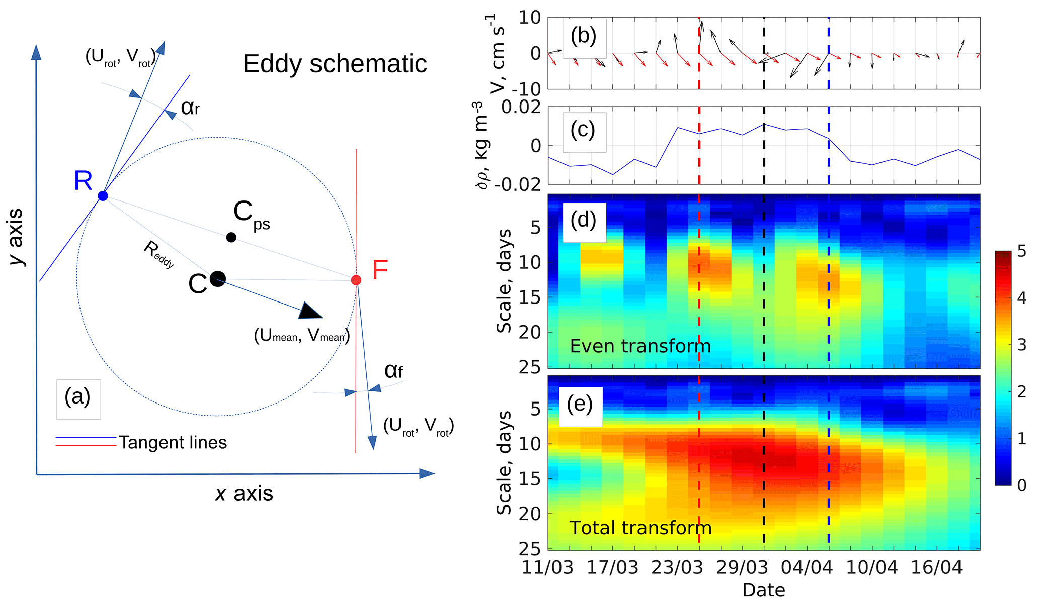
Figure 3(a) Schematic of an idealized eddy on a horizontal plane. F, R, C, and Cps points indicate the frontal and rear edges and the “true” and “pseudo” centers of an eddy, respectively. Umean and Vmean are the velocity components of the low-frequency current. Urot and Vrot are the rotational velocities at the frontal and rear edge of the eddy. αf and αr are angles between the vector of rotational currents and tangent lines at the frontal and rear borders of the eddy. An FR segment shows the trajectory by which the eddy passes through the mooring. Also shown are (b) vectors of rotational (black) and mean (red) current, (c) density anomalies, and (d) even and (e) total wavelet transformations of velocities from the MMP instrument in the Atlantic Water temperature core (254 m) at mooring M1f during the passing of a cyclonic eddy in March–April 2009. The frontal and rear eddy edges identified by even wavelet transformations are marked by red and blue dashed vertical lines, whereas the black vertical line associated with the maximum of the total wavelet transformation shows the time when the eddy “pseudo” center was at the mooring site. All wavelet transforms are in units of normalized variance.
Further, we calculated the complex rotational wavelet of complex Urot+iVrot. Two consequent extrema of even wavelet transforms – the real part of complex-valued wavelet transforms applied to complex-valued time series (see Lilly et al., 2002, for details of rotary wavelet decomposition for even and odd components) – indicate the reversal direction of currents at the frontal and rear edges of the eddy. Note that in this study, the “frontal” edge of the eddy is identified as that which passes the mooring site earlier in time (see Fig. 3 for an example). These reversal currents enable us to distinguish between the eddy passing and the unidirectional advection by the boundary current of temperature and salinity anomalies formed, for example, from upstream current meandering. Based on tests with idealized Rankine and Gaussian vortices, Lilly et al. (2002) concluded that the suggested pattern of wavelet spectra in eddies with two consequent extrema of the even wavelet transforms is invariant to the direction of the advecting flow and is not sensitive to the location of the slice by which eddies pass through the mooring site.
To avoid the false identification of eddies with this method, each eddy-like event was examined visually to verify that wavelet-based indicators coincide with an eddy. In addition, eddy-like events with rotational current speed less than the instrumental accuracy were eliminated from further analysis.
The separation of eddies and waves – e.g., long-period (>24 h) tidal and/or Rossby waves – with similar wavelet patterns can be difficult, however (Lilly et al., 2003). We approach this problem by also applying wavelet analysis to temperature and salinity records from the MMP. This approach is based on the assumption that mesoscale eddies carry temperature and salinity signals corresponding to their origin, whereas water transport associated with long waves is small, and temperature and salinity show signatures of local (eddy-unrelated) waters (LeBlond and Mysak, 1978; Chelton et al., 2011). For every level at which a potential eddy was identified, we calculated advective temperature and salinity changes δ(T, S), which can be induced by a local long-period wave of the same speed.
where τ is the time required for the eddy to pass through the mooring site, and is the strongest current speed anomaly in the eddy.
In these estimates, we used temperature and salinity gradients ∇(T, S) at the M1f mooring site derived from the climatological distributions for the 2000s (see Sect. 4.1 for details). Taking into account that the climatological gradients are usually smaller in comparison to those measured at synoptic timescales, we doubled δ(T, S) and used them as thresholds in our analysis. Specifically, all eddy-like events with temperature and salinity anomalies below these thresholds were eliminated from further consideration. Note that this additional criterion reduced the total number of eddy-like events for all observational levels by about 10 %, but kept unchanged the number of identified eddies within the M1f mooring record. This approach provides us with the assurance that the identified mesoscale features cannot be generated by local waves.
We estimated eddy rotational direction (polarization) using decomposed velocities at moorings. From these velocities, we derived polarization for every level of eddy-occupied mooring records by calculating the sign for vector products from the mean velocity of eddy advection (i.e., the “mean” current) and currents at the eddy's leading edge. This method of polarization evaluation is insensitive to which part of the vortex (i.e., central or peripheral) was observed. For additional assurance, we controlled the conservation of eddy polarization at both edges of the identified eddies. To ensure the identified eddy has the same polarization at the rear boundary of the eddy, we calculated an additional vector product using rotational velocities at the rear eddy edge. In the case of conservation of the polarization, the products at the frontal and rear eddy's edges have opposite signs, indicating the reversal of current direction.
The typical horizontal size of eddies (eddy radius, Re) was further estimated, assuming eddies are Rankine vortices with a circular shape and weak current divergence inside their bodies – see, e.g., Padman et al. (1990) and Bebieva and Timmermans (2016). The assumption of circular eddy shapes implies an orthogonal direction for rotational currents at the eddy edges toward a radius vector from the eddy center (see Fig. 3a for the idealized schematic of an eddy). With the additional assumption that the advection speed (Umean, Vmean) of an isolated Rankine vortex through the mooring site is constant, we can estimate Re at every depth level of the available observations by minimizing the average angle (αmean) – between the rotational current and tangent vector at the frontal (αf) and rear (αr) edges of the eddy – as a joint function of Re and the position of the eddy center (Fig. 3a). In the case of Rankine vortices with cyclonic or anticyclonic polarizations, all these angles tend to zero. That is, we minimize the error between the directions of idealized eddy (Rankine vortex) velocities and observations at the eddy edges (at the F and R points as shown in Fig. 3a). Similar to the routine proposed by Bebieva and Timmermans (2016), the iteration procedure employed involves an initial guess at the eddy center location (for the point C), which is repeated for all possible combinations of Re and the eddy center location until solutions converge. Since the algorithm seeks the position of the physical eddy center, and not the eddy's “pseudo center” (we use the term “pseudo” since the physical or “true” eddy center does not necessarily pass through the mooring site), its convergence ensures that our estimates of Re are insensitive to the trajectory of each particular eddy relative to the position of the mooring and thus to what part of the eddy was covered by observations.
Velocity records at both moorings reveal multiple events of strong current rotation, when flow changes its direction more than 90∘ over a short (from 4 to 15 days) period of time. These events are evident, for example, in a series of current vectors at the M1f mooring (Fig. 2, red marks), at the level of the AW temperature core (254 m), and at the deepest observational level (780 m), and they likely indicate the passage of eddies through the mooring site.
3.1 Wavelet-based identification of eddies
Given the large number of potential eddy events in the current vector time series, we implemented a semiautomated method for identifying them. We illustrate this method with an example of a cyclonic eddy captured at M1f between 25 March and 6 April 2009 (Fig. 3). In this example, we applied decomposition of the velocity series for the mean (i.e., eddy-unrelated) and rotational (i.e., eddy-induced) currents, as described in Sect. 2.2 and in the Supplement. Following Lilly et al. (2002, 2003), the local maximum of total wavelet power indicates when the eddy's “pseudo center” passed the mooring location (Fig. 3, see black dashed lines). Localization of the eddy's pseudo center allows for the accurate evaluation of water properties in proximity to the eddy core. Maxima of the even component of the wavelet transform (shown by red and blue lines in Fig. 3) indicate the times when frontal and rear eddy edges pass the mooring position. The eddy edges match in time with the strongest rotational current (Fig. 3b). The time difference between the passing of frontal and rear eddy edges provides an estimate of the overall duration of the eddy event.
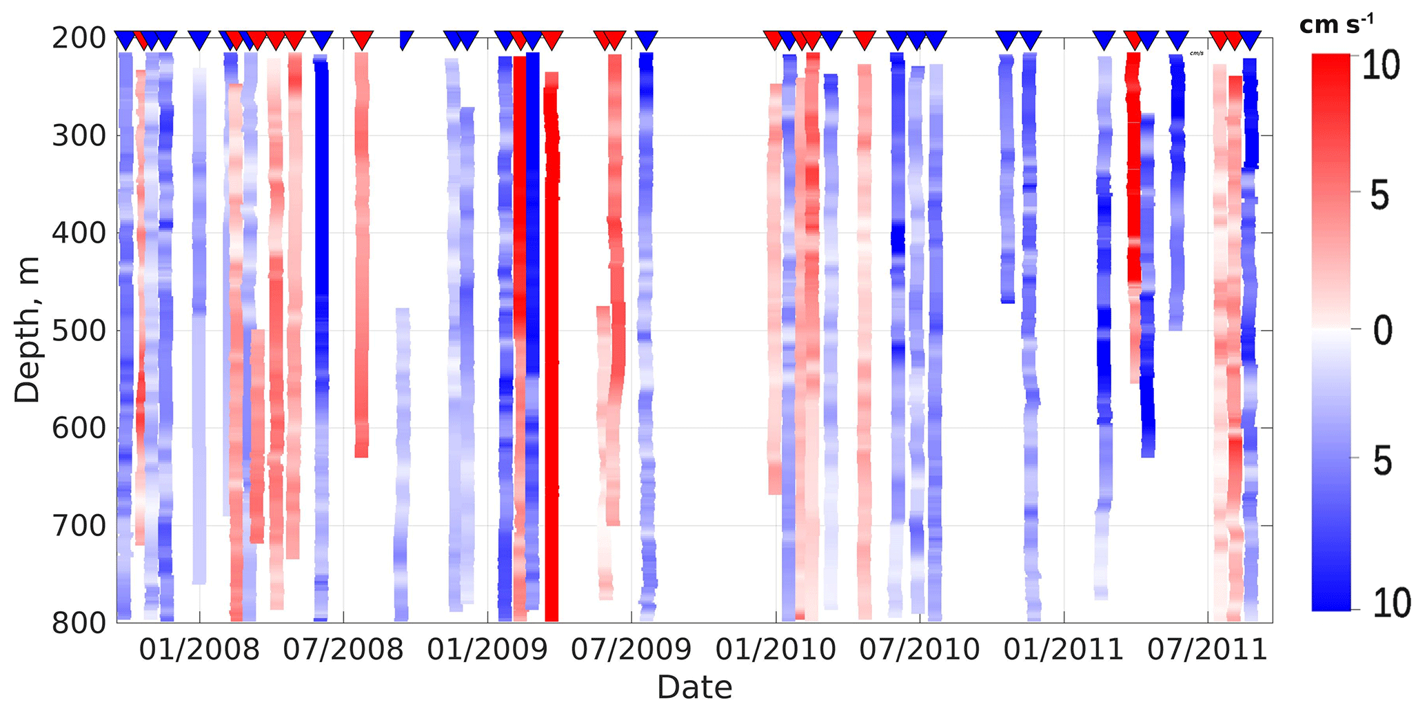
Figure 4Results of wavelet-based identification of eddies using the MMP record at the M1f mooring over the Laptev Sea continental slope in 2007–2011. Each vertical color stripe represents a single eddy. Red is used for anticyclonic rotation; blue is used for cyclonic rotation. Color intensity shows the rotational speed of eddies (cm s−1). Color triangles on top of the panel indicate the time when an eddy “pseudo” center passes the mooring site.

Figure 5Results of wavelet-based identification of eddies using two ADCP records at the M1g mooring over the Laptev Sea continental slope in 2009–2011. Each vertical color stripe represents a single eddy. Red is used for anticyclonic rotation; blue is used for cyclonic rotation. Color intensity shows the rotational speed of eddies (cm s−1). Color triangles on top of each panel indicate the time when an eddy “pseudo” center passes the mooring site.
We identified more than 350 eddy-like features in the wavelet transforms within the 4-year-long MMP record and over 50 events during the shorter ADCP records, wherein each feature is generally identified simultaneously at several adjacent depth levels (Figs. 4, 5). Features with vertical extents less than 10 m (five adjacent MMP levels or three ADCP levels) were then eliminated, leaving 41 and 23 eddy-like features within the M1f and M1g mooring records for the following analyses, respectively. We interpret the remaining features as mesoscale eddies, occupying substantial (∼20 %) fractions of the M1f (∼4 years) and M1g (∼22 months) time series. On average, about one eddy passed through the mooring site every ∼30 days. Colored marks appear at the top axis to show the time when the eddy “pseudo center” was at the mooring site (see Figs. 4, 5). We also calculated intervals between the frontal and rear edges of every eddy that crossed the mooring site. For both moorings, the average time each eddy was at the mooring site was about 7 days, suggesting the identified eddies were resolved sufficiently well by our daily and bi-daily mooring observations after low-pass filtering at 30 days.
The frequency of identified eddies was unevenly distributed over time. We found only five eddies for the 8-month period between April and December 2009 in the M1f (MMP) record (Fig. 4). Weakened eddy activity coincided in time with a large-scale change in the thermohaline state in the EB and was accompanied by anomalous westward flow of the Arctic Circumpolar Boundary Current (ACBC), for which the typical direction is eastward (see Pnyushkov et al., 2015 and their Fig. 12 for details).
Over some other time intervals, eddies were closely packed in space, with time between two consequent eddies comparable with the time during which an eddy is advected though the mooring site (e.g., January 2009 to March 2010 at mooring M1f and August 2009 to March 2010 at mooring M1g; see Figs. 4, 5).
Summarizing this section, we note that, on average, mesoscale eddies crossed mooring locations once per month, though there were periods when eddies were observed much more frequently (up to three eddies per month). The typical time during which an eddy was captured by mooring observations was about 1 week, but with modulation of eddy presence at this site by large-scale changes in the ACBC. In the next section, we assess general properties of eddies and their role in water mass transformations.
3.2 Properties of mesoscale eddies
3.2.1 Vertical extent
Eddies were identified in all parts of the water column covered by observations, including the AW layer and halocline (Figs. 4 and 5). The vertical extent of eddies was often within the depth range covered by MMP or ADCP observations. However, the height of 26 out of 41 eddies identified in the MMP record from the M1f mooring extended beyond the ∼600 m range covered by observations (Fig. 4). At the M1g mooring site, 18 out of 23 eddies extended beyond the 77–340 m depth range (Fig. 5). Relatively high rotational speed (up to 13 cm s−1) at the uppermost 77 m depth level at the M1g mooring site suggests that these eddies may extend well above this level, through the CHL to the base of the SML.
In the part of the deep EB sampled by ice-tethered profiler (ITP) observations during 2003–2014, Zhao et al. (2014) found mesoscale eddies within the halocline and intermediate layer, roughly in the 50–200 m depth range – the focus layer for their study. Eddies generally occupy a similar depth range in the Canada Basin (Timmermans et al., 2008; Spall et al., 2008; Kawaguchi et al., 2012). Our analyses of data from the Laptev Sea slope show that eddies can frequently be found significantly deeper, including deeper parts of the AW layer.

Figure 6Probability distribution function of eddy radii (a), rotational current speed (b), amplitude of isopycnal displacement (c), and relative vorticity (d) estimated using MMP observations at mooring M1f. Dotted lines on the panels indicate the 95 % confidence interval estimated by the bootstrap method. Red is used for anticyclonic eddies; blue is used for cyclonic eddies.

Figure 7Probability distribution function of eddy radii (a, b), rotational current speed (c, d), and relative vorticity (e, f) estimated using ADCP records collected at 125 m (a, c, e) and 290 m (b, d, f) at mooring M1g. Dotted lines indicate the 95 % confidence interval estimated by the bootstrap method. Red is used for anticyclonic eddies; blue is cyclonic eddies.
3.2.2 Eddy polarization
At mooring M1f, the 41 eddies (Fig. 4) consisted of 24 cyclonic (anticlockwise-rotation) events (58 % of the total) and 17 anticyclonic (clockwise-rotation) events (42 %). Approximately the same ratio of eddy polarization was found at mooring M1g, with 12 out of 23 eddies (or 52 %) being cyclonic. This almost equal partitioning of eddies between cyclonic and anticyclonic is in contrast with the findings by Woodgate et al. (2001), who reported a larger amount of anticyclonic eddies compared to cyclonic eddies at the Lomonosov Ridge, as well as Zhao et al. (2014), who found anticyclonic predominance for halocline eddies in the deep EB. We cannot explain this difference in ratios between cyclonic and anticyclonic eddies at the EB slope and in the deep Eurasian and Canada basins.
3.3 Eddy radii
Estimated eddy radii at M1g and M1f varied from 3 to 27 km, with average values of 12.2±0.6 and 11.5±0.1 km, respectively, where the cited errors are the standard errors of the mean. Probability distribution functions (PDFs) for Re are skewed and differ significantly for different instruments, depths, and eddy polarization (Figs. 6–7). The most common eddies have radii of ∼6–10 km, smaller than the mean eddy radius and consistent with the first baroclinic Rossby radius of deformation (Rd) estimated for the eastern EB (Rd∼7 km; Chelton et al, 1998; Nurser et al., 2014; Zhao et al., 2014). For the ADCP instrument that sampled the 77–125 m depth range at M1g, we found small differences in the probability density for small and large (>20 km) radii (Fig. 7a, b) so that the inferred PDF is more uniform than that derived from the MMP record (Fig. 6). However, the limited number of originally identified eddy-like events (21 individual eddies) leads to large uncertainty in this distribution. We quantify the robustness of our PDFs by estimating the 95 % confidence intervals with a bootstrap method that uses the range between the upper and lower 2.5 percentiles for each gradation of eddy radii estimated from 1000 randomly generated subsets (Davison and Hinkley, 1997). The same method to estimate the 95 % confidence interval of the PDF was implemented for all properties of mesoscale eddies (e.g., rotational current speed, relative vorticity, isopycnal displacement, and others).
The close estimates of the most common Re∼8–10 km and Rd ∼8 km, derived using in situ CTD observations over the Laptev Sea slope during the mooring deployment and recovery and in Fram Strait in 2009 (CTD profiles are available from the https://pangaea.de/ (last access: May 2015) website; https://doi.org/10.1594/PANGAEA.753658), suggest that baroclinic instability is the most likely mechanism for eddy formation. Barotropic instability is not as important for eddy generation for these areas (i.e., Fram Strait and the central Laptev Sea slope; see Teigen et al., 2011, for a discussion).
Uncertainties about estimates of Re were evaluated using a Monte Carlo sensitivity test. We added a uniformly distributed white noise to the rotational current velocities at the eddy edges, imitating the impact of instrumental errors and smaller-scale oceanic variability in observations of current velocities. Using the modified rotational current, we recalculated Re, repeating this calculation 20 times for every observational level spanned by the eddy to gain reliable statistics. Derived extrema (minimum and maximum radii) provide an uncertainty interval for each eddy to help evaluate the quality of radius estimates. An average accuracy for the described method, estimated as the range of the uncertainty interval in experiments with identified eddies at M1f in 2007–2011, was ∼1.8 km.
3.4 Rotational current speed and eddy-induced isopycnal displacement
After decomposing mooring-based series of currents for the mean current and rotational current anomalies fit to idealized Rankine vortices, we can estimate maximum rotational speed (Vrot) at the edges of each eddy. By combining Vrot with estimates of eddy radius Re (previous section), we can now evaluate the relative vorticity of eddies as . The observed eddies have significant rotational current speed and low relative vorticity (small Rossby numbers; Ro , where f is the Coriolis parameter). The maximum value for Vrot was ∼17 cm s−1, and the mean value for all 64 eddies was ∼5 cm s−1; the corresponding mean Rossby number was ∼0.05. The extreme and mean values for Vrot differ insignificantly between cyclonic and anticyclonic eddies so that the derived statistics for Vrot are mostly insensitive to eddy polarization (Figs. 6–7). Low Ro values (≪1) suggest a dominant role of geostrophic balance for eddies at the Laptev Sea slope.
Maximum eddy rotation speeds are comparable with the long-term mean current speed of 4–5 cm s−1 at the Laptev Sea continental slope (Pnyushkov et al., 2015). Higher values of the rotational speed were reported for eddies found in the Canada Basin (Krishfield et al., 2002; Pickart et al., 2005; Timmermans et al., 2008; Kawaguchi et al., 2012). For example, Kawaguchi et al. (2012) reported Vrot as large as 57 cm s−1 for a large-scale (∼60–70 km in diameter) eddy observed at the boundary of the Chukchi and Beaufort seas, with an associated value of Ro ≈0.1. Higher rotational speeds were also found within Arctic halocline eddies, in which Vrot varied in the range of 5–40 cm s−1 (Zhao et al., 2014). Vertical distribution of the rotational speed in eddies is not uniform, with larger rotational velocities in the upper ∼500 m layer (Figs. 4, 5). However, for some eddies at the M1f mooring (e.g., in May–July 2010), significant changes in rotational speed with depth are likely due to the contamination of the eddy signal by sub-mesoscale current variability (e.g., internal waves, unfiltered baroclinic tides), which are not fully resolved by our MMP and ADCP records.
Advection of mesoscale eddies through the mooring sites analyzed here was accompanied by potential density anomalies relative to the ambient waters. These anomalies are a combination of isopycnal displacements associated with the rotational velocities of the eddies and anomalous water mass characteristics associated with the advection of the eddies from remote sources where ambient T–S characteristics are different from those at our moorings. In accordance with a quasi-geostrophic theory (see Pedlosky, 1990 for details), anticyclonic eddy formation is accompanied by downward displacement of isopycnals and elevation of the sea surface. In cyclonic eddies, the situation is reversed. In agreement with the theory, we found that cyclonic and anticyclonic eddies at M1f were accompanied by doming and lowering of isopycnal surfaces and a corresponding positive–negative density anomaly inside their cores. On average, isopycnals change their vertical position by 15–20 m as the eddy passes the mooring (Fig. 6). The lifting or lowering of the isopycnal surfaces and the density anomaly at a specific depth can be used as a “first-guess” criterion to identify eddies crossing the mooring; this is similar to how eddies are identified in ITP records (e.g., Timmermans et al., 2008; Zhao et al., 2014). However, joint wavelet analysis of density and velocity series at M1f suggests that ∼20 % of isolated density anomalies were not accompanied by corresponding increases in rotational velocities.
The long lifetime of eddy structures is a known property of oceanic eddies. For example, some Gulf Stream rings and thermocline lenses are able to survive in the ocean for a few years (e.g., Cheney and Richardson, 1976; McWilliams, 1985; Olson, 1991; Richardson et al., 1991). Arctic Ocean eddies may also travel several thousand kilometers from their origins over a period of several years, preserving the properties of water trapped inside their cores (e.g., Newton et al., 1974; Manley and Hunkins, 1985; D'Asaro, 1988). Dmitrenko et al. (2008) analyzed temperature and salinity distributions in the core of a warm AW eddy observed at a mooring over the Laptev Sea slope and concluded that it was formed in the vicinity of St. Anna Trough – i.e., ∼1100 km west of the mooring site.
We used comparison of climatological and eddy profiles of water temperature and salinity to identify the source regions for eddies observed in the eastern Eurasian Basin. For that, we quantified the similarity between temperature and salinity profiles and climatology. We developed a combined temperature–salinity criterion, Ji, j, specified in an isopycnal vertical coordinate, σ:
where σ1 and σ2 are the potential density of the lower and upper boundaries of the eddy, respectively; Teddy(σ) and Seddy(σ) are temperature and salinity measured inside the eddy core; and are the climatological temperature and salinity; i and j are the longitudinal and latitudinal indices of the climatological profiles; and SDT and SDS are standard deviations within temperature and salinity profiles estimated from the eddy core. The normalization of temperature and salinity terms using SDT and SDS accounts for the uneven contributions to Ji, j from temperature and salinity differences. The minimum for Ji, j indicates that climatological temperature and salinity profiles from the site at coordinates (i, j) have maximal similarity with profiles inside the eddy core, in which case the eddy has potentially originated in the same area where the climatological profiles were taken.
4.1 Two potential sources of eddy formation in the EB
For analysis of potential eddy sources, we utilized an extensive dataset of temperature and salinity observations collected in the Arctic Ocean over the 2000–2010 period. Previous analyses of this dataset include studies of long-term changes in the thermohaline state of the EB and evaluation of interannual changes in the boundary current in the EB (Polyakov et al., 2008, 2012; Pnyushkov et al., 2015). Those papers provide a detailed description of this dataset, which includes multiple ship-based CTD surveys complemented by ITP (http://www.whoi.edu/page.do?pid=20756, last access: May 2015) observations, providing extensive year-round measurements of temperature and salinity in the upper ∼800 m ocean layer. The total number of thermohaline profiles collected in this dataset for the EB is ∼15 000 (see Polyakov et al., 2012, and their Fig. 2 for a detailed map with data coverage). These observations were averaged within a 150 km radius around nodes of a regular grid with 0.25∘ spatial resolution to provide climatological temperature and salinities for 2000–2010. Each climatological value was accompanied by a standard error of the mean, which was used in our analysis to assess uncertainties of eddy origin identification (see Sect. 4.2 for details).
The described method for finding eddy origins was applied to eddies found in the mooring M1f record, for which we have concurrent measurements of temperature and salinity profiles inside the cores of eddies. For eddies passing through this mooring, we identified two distinct sources of eddy origin: one in the region of Fram Strait and the other at the continental slope of Severnaya Zemlya Archipelago (Fig. 8). In the Fram Strait area, roughly 2000 km upstream of the mooring sites, potential eddy origins were concentrated near the Yermak Plateau, the region north of Spitsbergen with strong mesoscale ocean dynamics (e.g., Hunkins, 1986; D'Asaro and Morison, 1992; Padman et al., 1992; Muench et al., 1992; Våge et al., 2016; Crews et al., 2018), and further along the continental slope between Spitsbergen and Franz Josef Land. Available mooring observations in this region show strong variability of currents expressed in terms of standard deviations of the velocity components (e.g., Pnyushkov et al., 2015). This strong variability likely indicates current instability similar to the baroclinic instability of the West Spitsbergen Current in Fram Strait (Teigen et al., 2011).
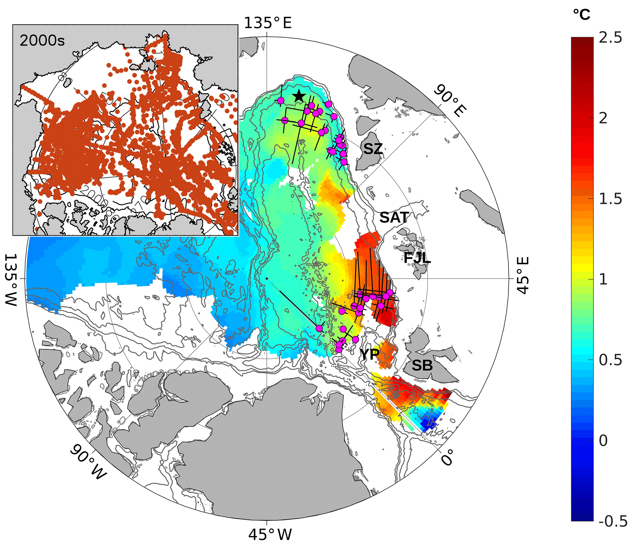
Figure 8Results of the identification of eddy origins using the M1f mooring record (2007–2011). Pink circles show the locations of climatological profiles with maximal temperature and salinity similarity with profiles observed inside the eddy cores. The black star shows the M1f mooring position. Climatological temperature (∘C, color bar) for the 2000s averaged within the 200–800 m layer is shown by color (white spots indicate no data). Black crosses with uneven crossbars at the center of each origin indicate estimated errors of eddy origin position (longer crossbars indicate larger errors in the eddy origin position). Note that for some eddies, confidence intervals are small and not distinguishable at this scale. Gray contours show isobaths. SB, YP, FJL, SAT, and SZ denote Spitsbergen, Yermak Plateau, Franz Josef Land, St. Anna Trough, and Severnaya Zemlya, respectively. Data coverage of oceanographic profiles used in the 2000s climatology is shown in the insert.
The second area of eddy origin is located much closer to our moorings, near the unstable density front that is formed by the confluence of Fram Strait and Barents Sea AW branches north of the Severnaya Zemlya Archipelago (Schauer et al., 1997).
In addition to the results of the method employed in Eq. (1), we compared temperatures and salinities inside the identified eddies with those estimated using the climatology for the 2000s (Figs. 9 and 10e). The evident similarity between the T–S plots derived with T and S inside eddy cores and climatological temperatures and salinities averaged for the nodes of potential eddy origins (pink dots in Fig. 8) likely suggests that our separation of eddy origins for two sources is robust.
4.2 Quality of eddy origin identification
The mean temperatures and salinities inside the eddy cores ( and ) and those in the eddy origins ( and , derived from the climatology) were used to estimate the quality of eddy origin identification and uncertainty in their positions. We found linear relationships between and and between and , with slopes of best-fit lines close to 45∘ and high linear correlations ( for both T and S; significant at a 95 % confidence level) (Fig. 9). To estimate how the temperature difference , which we interpret as a measure of uncertainty, affects estimates of the position of eddy origin, we found the minimal distance at which climatic temperatures differ by ΔT from (Table 1). Since the analysis of eddy origins was performed for mooring M1f and not for M1g, we provide limited statistics for 41 eddies only. We repeated the same routine for salinity. We found that the contribution of salinity to the uncertainty of eddy sources is comparable to the contribution of temperature (see Figs. 8 and S1). These equal contributions suggest that when using Eq. (1) we cannot rely solely on temperature anomalies inside eddy cores to identify eddy origins.
Table 1Errors of eddy origin identification (in km) estimated using differences between temperature and salinity in eddy cores and climatological profiles.
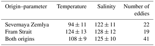
Averaged separately for the two areas of eddy formation (i.e., for Fram Strait and Severnaya Zemlya slope), these errors suggest that eddy origins were estimated with approximately equal accuracy of about 100 km for both sites. These errors are significantly (by a factor of 4) larger than the uncertainty for eddy origins caused by errors in 2000s climatology temperatures and salinities given by standard errors of the climatological mean (see Fig. 8, black lines, for example). However, the uncertainties are much smaller than the separation (∼1400 km) of the eddy source regions at Fram Strait and the Severnaya Zemlya slope, indicating that the partitioning of eddies between the two sources is robust. This partitioning is also insensitive to our choice of utilized climatology temperatures and salinities. For example, we found very similar partitioning of eddy sources when we repeated the identification of eddy origins using a global polar hydrographic climatology dataset, which synthesized observations prior to the 1990s (not shown, Steele et al., 2001). However, we note that the approach utilized for eddy source identification does not take into account the transformation of Teddy and Seddy during propagation from the eddy origin to the mooring site at the Laptev Sea slope. The cooling and freshening associated with the progression of waters (including eddies) from the source region into the ocean interior suggests the actual eddy origins may be located further upstream from the identified source areas (probably in Fram Strait and St. Anna Trough).
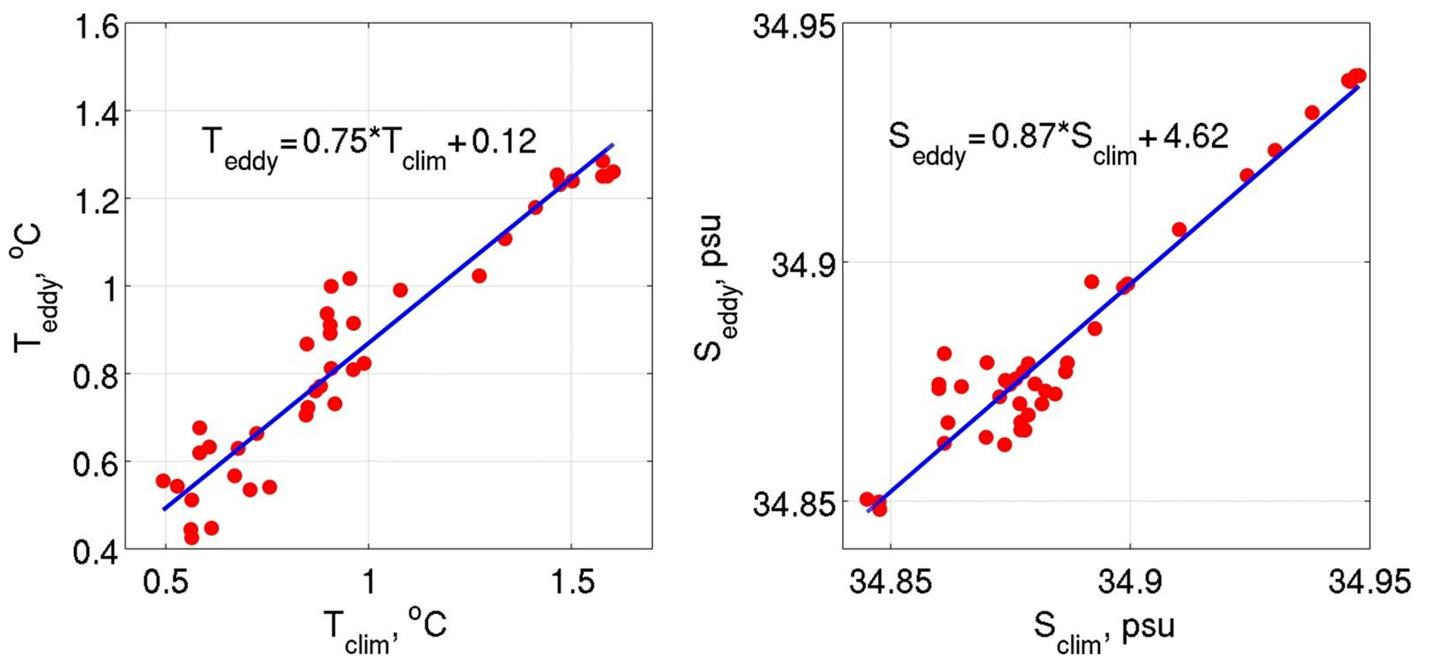
Figure 9Mean temperature ∕ salinity (Teddy∕Seddy) inside the eddy core versus climatological temperature ∕ salinity (Tclim∕Sclim) at the eddy origin. Each temperature ∕ salinity was averaged within the water layer spanned by the eddy.
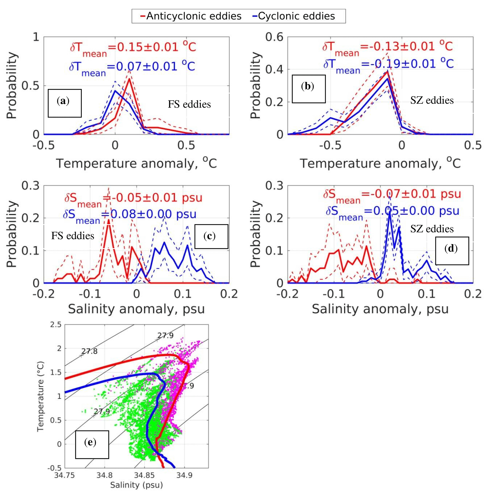
Figure 10The probability distribution function of temperature (a, b) and salinity (c, d) anomalies inside cores of Fram Strait and Severnaya Zemlya eddies and the corresponding T–S plot (e). Temperature and salinity anomalies were estimated for the layer above the Atlantic Water temperature core relative to the temperatures of ambient waters in the same layer. Dotted lines in panels (a–d) indicate the 95 % confidence interval estimated by the bootstrap method. Magenta dots in (e) are used for FS eddies; green dots are used for SZ eddies. Red and blue solid lines show the T–S plot derived using climatological temperature and salinities averaged for the Fram Strait and Severnaya Zemlya areas. Black solid lines show isopycnals.
In addition to the along-slope transformations of Teddy and Seddy, short-term, seasonal, and interannual variability in hydrography in the EB also affect the results of eddy source identification. We quantify these effects using standard deviations for temperature and salinity as a measure of variability calculated using the collected Arctic Ocean observations over the 2000–2010 period. For sites of eddy origins (Fig. S2; pink dots), we estimated the minimal distance at which climatic temperatures and salinities differ more than 1 standard deviation, as derived within a 150 km radius around the node. The calculated distances were comparable to those derived with ΔT (see Fig. 8 for comparison). For instance, the mean error for the Fram Strait eddies was 96 km, ∼28 km smaller than the mean error calculated using ΔT. For the Severnaya Zemlya eddies, the mean difference was even lower (∼22 km). We repeated the same analysis using standard deviations for salinity; the estimated mean errors for both source regions do not exceed those evaluated for temperature. Summarizing, even though particular uncertainty regarding source location for any individual eddy may be substantial (up to 220 km), this is significantly smaller than the distance from Fram Strait to the Severnaya Zemlya slope – the two potential areas of eddy formation in the EB – suggesting the robustness of the partitioning of eddies between the two sources.
4.3 Temperature anomalies inside eddies
The lateral advection of waters isolated inside the eddy cores by the ACBC may affect the heat and salt balance of the eastern EB, as well as more remote regions located downstream along the pathway of the boundary current. For example, an analysis of Fram Strait eddies shows these eddies carry anomalously warm water in comparison with the ambient local waters observed at M1f during 2007–2011 (Fig. 10). The mean temperature anomaly estimated for the layer above the AW temperature core (i.e., above the 350 m depth level) was ∼0.1 ∘C, with the strongest temperature anomaly in this layer exceeding 0.5 ∘C. An even higher (up to 1 ∘C) temperature anomaly was reported by Dmitrenko et al. (2008) for a mesoscale eddy observed in February 2005 at a mooring over the Laptev Sea continental slope at the same position as the M1f mooring site. In our record, such strong temperature anomalies in the Fram Strait eddies are rare, and only ∼16 % of them exceed 0.2 ∘C.
In contrast to Fram Strait eddies, Severnaya Zemlya (SZ) eddies carry anomalously cold water inside their bodies, while propagating along the continental slope of the eastern EB (see Fig. S3 for temperature, salinity, and potential density profiles inside the typical SZ eddy). For example, almost all (∼95 %) SZ eddies have negative temperature anomalies within the layer above the AW core. The average magnitude of the temperature anomaly (∼0.1 ∘C) in SZ eddies is similar (but of the opposite sign) to Fram Strait eddies. However, the most extreme anomaly magnitude in the set of observed SZ eddies is >0.8 ∘C, likely caused by smaller exchanges with ambient waters, while propagating from an origin fairly close to M1f. Evaluating statistics of temperature anomalies separately for cyclonic and anticyclonic eddies, we found no substantial differences in temperature anomalies in relation to eddy polarization for both eddy origins. This suggests that eddy rotation is controlled mostly by salinity (see Fig. 10c, d) to form a positive–negative density anomaly in cyclonic and anticyclonic eddies, in agreement with the geostrophic balance. Moreover, these anomalies are formed mostly due to transport of trapped waters rather than local vertical advection. Otherwise, stronger differences between temperature anomalies caused by a different pattern of vertical circulation in cyclonic and anticyclonic eddies are expected. In agreement with our finding of the dominant role of salinity for density anomalies inside EB eddies, the PDFs for density anomalies (not shown) look very similar to those calculated for salinity (Fig. 10c, d).
5.1 Vertical shear of velocities
In Sect. 3.4 we concluded that EB eddies have substantial rotational speeds comparable in magnitude to the mean speed of the ACBC at the mooring site. In addition, these eddies are sites of enhanced vertical shear. For example, we found an increase in squared shear by more than 1 order of magnitude during propagation of a cyclonic eddy through the M1f mooring between 25 March and 6 April 2009 (Fig. 11). The maximum for S2 in depth was found within the AW core (i.e., 250–270 m of depth), while the vertical position and magnitude of this maximum changed insignificantly during the passing of eddy edges and core. The value of S2 is vertically uniform below the AW core, though it still remains significantly larger than in the surrounding (eddy-free) waters (Fig. 11d).
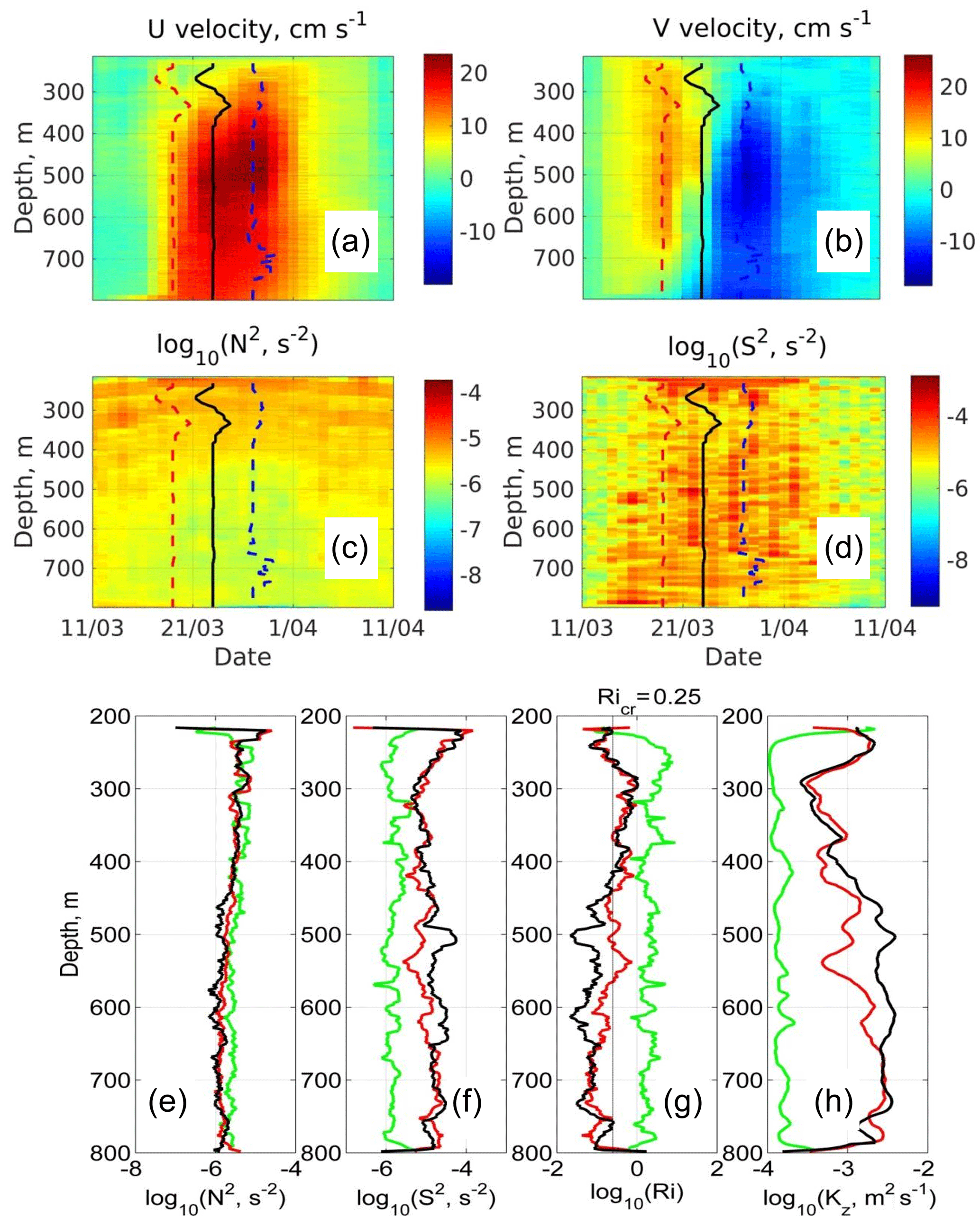
Figure 11Depth versus time distribution of eastward (U; a) and northward (V; b) velocities, squared buoyancy frequency (N2; c), and squared velocity shear (S2; d) inside a cyclonic eddy observed at mooring M1f in March–April 2009. Profiles of squared buoyancy frequency (e), squared velocity shear (f), Richardson number (Ri, g), and vertical diffusivity coefficient (Kz, h) at the frontal edge of a cyclonic eddy (red lines), in its center (black), and outside of an eddy (green). Kz values were estimated using the Pacanowski and Philander (1981) parameterization. Data shown in (h) were smoothed using a 21 m running mean for better visualization. The frontal and rear eddy edges and the eddy “pseudo” center in (a–d) are shown by red, blue, and black lines, respectively.
Increased velocity shear is evident within an eddy's core and also after the passing of the rear edge of an eddy, consistent with the gradual decay of rotational currents expected in a Rankine vortex outside the core of the solid-body rotation. The extension of eddy signatures beyond the period identified by our wavelet analysis suggests that the impact of eddies on ventilation of the surrounding waters may be larger than implied by our estimate of total time occupied by eddies (i.e., more than ∼20 % of the time spanned by our records; Sect. 3).
5.2 Estimates of vertical diffusivity coefficients
The observed increase in vertical velocity shear in eddies suggests that they may produce enhanced vertical mixing and thereby contribute to ocean ventilation at the EB slopes. We evaluated the potential influence of eddies on ocean mixing by estimating vertical diffusivity Kz, following Pacanowski and Philander (1981), who devised a commonly used parameterization based on the statistical relationship between Kz and the gradient Richardson number. In this parameterization, Kz is estimated as
where α=5, n=2, υb is the background diffusivity coefficient (typically presumed to be in the range 10−5–10−4 m2 s−1, and m2 s−1 is the diffusivity at neutral stratification.
Using Eq. (1), we estimate that turbulent mixing increased during the time of the eddy passing through the mooring. Inside the eddy core, Kz is about m2 s−1, approximately an order of magnitude larger than the chosen background diffusivity coefficients in eddy-free waters ( m2 s−1; Fig. 11). Above the AW core, the pattern of Kz follows S2, consistent with the variability of S2 dominating over the variability of N2 in the calculation of Ri. There is a gradual increase in Kz in the layer below the AW core (i.e., below ∼300 m of depth) so that Kz has a local maximum at ∼540 m of depth (Fig. 11f). The increase in Kz with depth in this layer is due to the gradual reduction in background stratification with increasing depth, while S2 is nearly constant so that Ri decreases, leading to higher parameterized Kz (Fig. 11a, b). An increase in Kz in the layer between 100 and 500 m was also found, for instance, at the North Pole Environmental Observatory moorings (∼90∘ N) by Guthrie et al. (2013), who utilized a collection of expendable current profiler measurements to estimate diapycnal mixing for several parts of the Arctic Ocean.
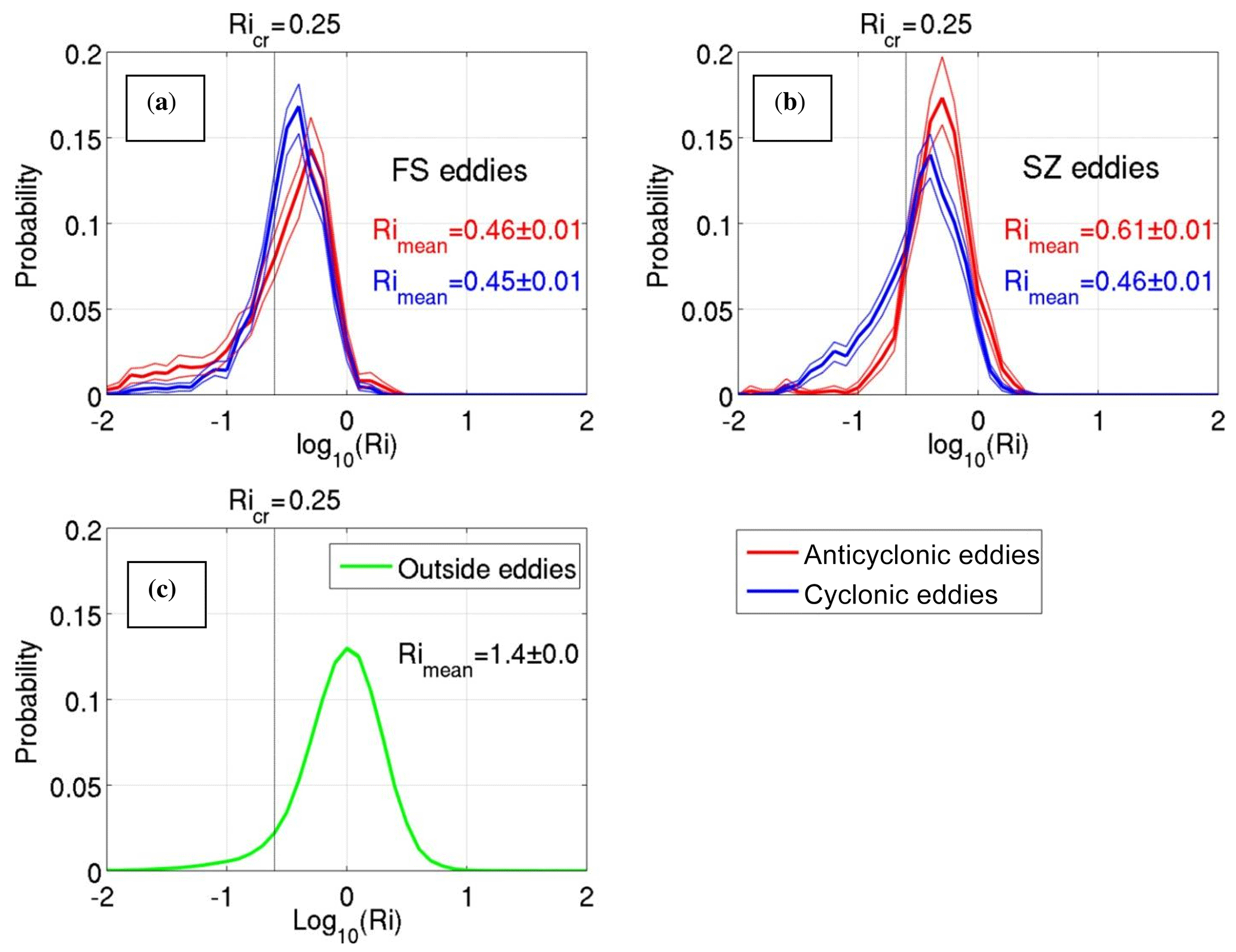
Figure 12Probability distribution function of Richardson numbers (Ri) estimated for Fram Strait (FS) eddies (a), Severnaya Zemlya (SZ) eddies (b), and using M1f mooring observations after eliminating identified eddy events (c). Vertical dashed lines indicate the critical Richardson number (Ricr), which separates areas of stable and unstable (turbulent) flow. Red and blue dotted lines indicate the 95 % confidence interval estimated by the bootstrap method. The 95 % confidence intervals in (c) are indistinguishable at these scales.
Below the AW temperature core, we found an extensive layer of low stratification ( s−2) between 450 and 750 m depths, which is several times weaker than the background stratification before and after eddy passing (Fig. 11a). We hypothesize that this layer of weakly stratified waters is a result of enhanced turbulent mixing in the eddy compared to ambient waters. Mixing in the layer above the AW temperature core (216–300 m) is also increased (as was identified by higher Kz). However, this intensity is not strong enough to cause complete mixing within that layer.
We extended estimates of Kz for the particular eddy described in the previous paragraph, with overall statistics for Ri at the mooring M1f for 2007–2011 (Fig. 12). For calculating these statistics, we used temperatures, salinities, and lateral velocity profiles averaged over 2 m vertical cells to estimate N2 and S2. The average Richardson number (Rimean =1.4) estimated for all levels during eddy-free periods is approximately 3 times larger than the average Ri found inside the Fram Strait (RiFram=0.45) and Severnaya Zemlya (RiSZ=0.51) eddies. Based on the Pacanowski and Philander (1981) mixing parameterization, these values for Ri suggest that Kz inside eddies is about 4 times larger than in the ambient ACBC. The similarity of PDFs for Ri values suggests insignificant differences in mixing rates between the Fram Strait and Severnaya Zemlya eddies.
The dependence of our estimates of mixing rates on the simplified empirical parameterization developed by Pacanowski and Philander (1981) suggests that the values of Kz shown in Fig. 11f may not be reliable. Thus, in addition, we estimated Kz using the Gregg (2003) parameterization, which is based on the theory of internal wave-to-wave interaction and includes fine-scale parameterizations derived from shear and strain characteristics. This analysis suggests an even stronger (about 2 orders of magnitude; not shown) increase in Kz in comparison with Kz in the surrounding waters. Based on these studies, we conclude that the increased level of mixing inside eddies relative to background ACBC is probably a robust feature, suggesting that mesoscale eddies may be important for diapycnal exchanges and that climate-related changes in eddy production rates and characteristics may play a role in the variability of time-averaged diapycnal fluxes.
The impact of eddies on vertical heat transport at the Laptev Sea slope was estimated by calculating eddy-induced vertical heat fluxes in the layer above the AW temperature core (i.e., above the 350 m depth level), where ρ and cp are the density and the specific heat of seawater, respectively. In these calculations, we utilized Kz derived in the identified eddies and vertical temperature gradients estimated at the M1f mooring site using the MMP temperature profiles. The derived vertical heat fluxes vary in a wide range from ∼0.01 to ∼6.3 W m−2 with an average value of 0.6±0.1 W m−2, which is 3 times larger than the heat fluxes in the ambient (eddy-unrelated) waters ( W m−2). However, with the available MMP record limited by a 216 m depth from the top, the fate of this eddy-induced heat surplus (0.4±0.1 W m−2) is not completely clear.
6.1 Properties of eddies at the Laptev Sea continental slope
Our analyses provide the most complete description of the structural characteristics of mesoscale eddies carried along the eastern EB continental slope with the ACBC. Although our observations are restricted geographically by the locations of two nearby moorings, the use of current velocity observations in addition to the hydrographic records has proven to be helpful for a description of eddies compared to previous studies based solely on observed temperature and salinity properties (e.g., Timmermans et al., 2008; Carpenter and Timmermans, 2012; Zhao et al., 2014).
Estimated eddy radii of the order of 10 km (Figs. 6–7) are similar to the first baroclinic radius of deformation, suggesting the generation of eddies by baroclinic instabilities. We note, however, that higher baroclinic modes, with smaller lateral scales than for the first baroclinic mode, may also contribute to eddy generation. Most observed eddies span the complete depth range of the measurement systems: ∼200–800 m of depth for the MMP at mooring M1f (Fig. 4) and ∼80–340 m of depth from the two ADCPs on mooring M1g (Fig. 5). Typical values of the inferred maximum rotation velocity in each eddy are ∼5 cm s−1 (Figs. 6–7), although rotational currents can occasionally exceed 15 cm s−1. The associated Rossby number (Ro) for these eddies is ≪1, indicating their dynamics as primary geostrophic. Eddy polarization is about equally divided between cyclonic (counterclockwise) and anticyclonic (clockwise) rotations.
The typical time for an eddy to pass through the mooring sites is about 1 week, with an average of about 1 month between eddies; that is, eddies are present in our records about 20 %–25 % of the time. These eddies are, however, unevenly distributed over the records, with time between two consequent eddies through the mooring varying from 4 to 150 days (Figs. 4–5). Various mechanisms may affect the frequency of eddy registration at the moorings. The weakened eddy activity between April and December 2009 at the M1f mooring was concurrent with large-scale changes in the thermohaline state of the EB, including the opposite signs of the eastward velocity component of the ACBC (see Pnyushkov et al., 2015 for details; Fig. 2c). An anomalous distribution of density in 2009 had a substantial effect on density-driven circulation in the eastern EB with low or even negative eastward ACBC transport and enhanced advection along the Gakkel Ridge. We speculate that the changes in the thermohaline state of the eastern Eurasian Basin are unlikely to modify the intensity of eddy generation (e.g., baroclinic instability of the ACBC), but alternate the pathway of eddy advection along the EB slope from Fram Strait or Severnaya Zemlya to the Laptev Sea slope. Seasonal and interannual changes in the cross-slope location of the ACBC core may also affect observed eddy variability at the specific cross-slope locations of our moorings.
Based on temperature and salinity anomalies in the eddy cores, we conclude the observed eddies at the Laptev Sea slope moorings are initially formed in two distinct regions of the eastern Arctic – in the vicinity of Fram Strait and north of Severnaya Zemlya (or St. Anna Trough), where the Fram Strait and Barents Sea branches of AW inflow meet (Fig. 8). However, we note that the utilized method of eddy origin identification likely failed once when the origin for one eddy was found at the Lomonosov Ridge near the North Pole. The statistical characteristics of the two types of eddy are, in general, comparable (Figs. 6–7); however, more of the large eddies (radius >20 km) observed at mooring M1f are anticyclonic than cyclonic (Fig. 6a).
Estimates of mixing rates from an empirical parameterization (Pacanowski and Philander, 1981) based on Richardson number suggest that mixing within eddy cores is about 4–10 times higher than in the ambient waters of the ACBC (Fig. 11f), primarily because of an increase in vertical velocity shear associated with eddies (Fig. 11d), which leads to much lower Richardson numbers (Figs. 11e and 12).
6.2 Comparison with previous studies of Eurasian Basin eddies
Our data are limited to depths below the uppermost depth bin of the upward-looking ADCP on mooring M1g (∼77 m), and our analyses are focused on the depth range encompassed by the subsurface layer of AW and the cold halocline. The only comparable prior study of eddies in the AW layer of the EB was by Woodgate et al. (2001), who used a collection of year-long velocity records from three moorings deployed over the Lomonosov Ridge in the eastern EB to summarize statistics for approximately 50 eddies. The set of eddies reported by Woodgate et al. (2001) differs from our set in the following ways. Over the Lomonosov Ridge, the polarization of EB eddies was predominantly anticyclonic (in about 80 % of the cases); this partitioning was roughly the same for both surface and deep-layer (>120 m) eddies. For deep-layer eddies, the observed vertical extent was large (often >1000 m), and eddies spanned the entire water column down to the seabed. The observed vertical extent was larger than in our observations; however, our measurements were limited by the sampling range of the MMP at mooring M1f.
Woodgate et al. (2001) suggested the eddies they observed over the Lomonosov Ridge originated at the confluence of the Fram Strait and Barents Sea branches of AW inflow, near the St. Anna Trough. This site is west of our identified eddy production area north of Severnaya Zemlya (Fig. 8), but is associated with the same general process of instability at a strong frontal boundary. We have not identified the reason why the partitioning of polarization is different at our site on the Laptev Sea slope than over the Lomonosov Ridge. In fact, it may be related to eddy dynamics at the intersection of the ridge with the continental shelf north of the Novosibirskiye Islands as the eddies are diverted northward by the ridge.
A more recent study of Arctic eddies by Zhao et al. (2014) identified several eddies in the “Eurasian water” in the Transpolar Drift Stream. That study focused primarily on the halocline, with the typical depth of the eddy cores being ∼50–80 m. These authors tentatively concluded that most Eurasian water eddies (34 of 39) were formed by surface buoyancy flux, with only five arising from instability of boundary currents. However, our analysis of the origins of AW eddies we observed on the Laptev Sea slope (Sect. 4, and Fig. 8) is consistent with eddy formation through baroclinic instabilities in the ACBC. All of the EB halocline eddies reported by Zhao et al. (2014) rotated anticyclonically, as expected for eddies formed by localized winter convection in the surface layers (Manley and Hunkins, 1985).
6.3 Eddy contribution to vertical transport of heat, salt, and nutrients
Even if the advective temperature anomalies within eddies are small (∼0.1 ∘C on average), eddies provide a mechanism for increased friction at the seabed and the ice base through the addition of eddy rotational velocities to mean flow. These velocities include cross-slope components that may bring AW periodically upslope to increase both the potential for mixing with shelf-modified water masses and the exposure of the upper layers of AW to mixing processes driven by surface buoyancy fluxes and wind stress. The eddies we observed at the Laptev Sea slope will presumably continue their path with the mean circulation around the EB, to be found later along the Lomonosov Ridge or even in the Canada Basin. We therefore expect that changes in eddy production rates (e.g., due to changing baroclinic stability of the ACBC) will affect thermohaline structure and mixing (benthic, ice–ocean, and perhaps isopycnal) throughout the EB, implying the need for accurate representation of eddy formation and dynamics in predictive ocean models.
6.4 Limitations of our analyses
The temporal resolution of our mooring records (1 and 2 days at moorings M1g and M1f, respectively) is adequate to resolve most eddies, which each take about 1 week to be advected past our moorings. This sampling is sufficient for coarse characterization of eddy scales, but is not adequate for detailed exploration of an eddy's internal structure. Analysis of eddy dynamics is further complicated by uncertainty in the path of the eddy's center relative to the mooring; while we assume that the eddy is circular, with eddy velocity always normal to the radius, we cannot validate this assumption with our mooring data.
Vertical resolution (∼2 m averages) of velocity, temperature, and salinity profiles at both moorings is too coarse to resolve small-scale processes that may be important for diapycnal mixing, including shear-driven instabilities and double diffusion. We therefore must rely on parameterizations based on large-scale flow characteristics to estimate mixing rates, including diapycnal diffusivity. We expect these parameterizations to correctly identify relative rates of mixing (e.g., higher diffusivity in eddy cores than in ambient water); however, absolute values for diapycnal fluxes may not be accurate. Thus, additional microstructure observations, similar to those reported by Padman et al. (1990) for a sub-mesoscale eddy in the Canada Basin, are required to improve our confidence in estimates of mixing rates.
6.5 Summary
Our study adds to the evidence that eddies of Atlantic Water in the EB, embedded in the ACBC, carry anomalous water properties along the eastern Arctic continental slope. The increased mean velocity due to the presence of eddies is an added potential source of mixing far from the original sources of the eddies and may also impact sea ice through additional friction at the ice–water interface and increased diapycnal fluxes from warm intermediate AW to the SML and eventually to the ice.
Our data from two moorings on the Laptev Sea continental slope do not allow us to investigate whether these AW eddies can carry significant heat into the interiors of the deep EB. Nevertheless, their presence suggests a pathway for this heat, which would provide a means for intermittent loss of the insulating effect of the cold halocline over the eastern Arctic Ocean. Assuming our parameterized estimates of increased diapycnal mixing within these eddies is robust, the eddies may play a role in maintaining some upward oceanic heat flux required to explain the mass balance anomaly of eastern Arctic sea ice (∼1 W m−2; Kwok and Untersteiner, 2011). Furthermore, this interpretation suggests that processes influencing the initial production of eddies could affect this upward flux to the surface, adding complexity to our understanding of how sea ice might respond to future large-scale changes in AW circulation.
All mooring data described in this paper can be accessed from the NABOS project website (http://nabos.iarc.uaf.edu/, NABOS, 2018).
The supplement related to this article is available online at: https://doi.org/10.5194/os-14-1329-2018-supplement.
AP carried out the identification and statistical analysis of mesoscale eddies. All authors contributed to the analysis and interpretation of the results and writing the paper.
The authors declare that they have no conflict of interest.
The authors thank the editor and two anonymous reviewers for assistance
in evaluating this paper. This study was supported by NSF grant
no. 1708427 (AP, IP) and no. 1702484 (LP). The mooring- and ship-based
oceanographic observations in the eastern EB were conducted within the
framework of the NABOS project, with support from the NSF (grants AON-1203473
and AON-1338948).
Edited by: Matthew Hecht
Reviewed by: two anonymous referees
Aagaard, K., Coachman, L. K., and Carmack, E. C.: On the halocline of the Arctic Ocean, Deep-Sea Res., 28, 529–545, 1981.
Aagaard, K., Andersen, R., Swift, J., and Johnson, J.: A large eddy in the central Arctic Ocean, Geophys. Res. Lett., 35, L09601, https://doi.org/10.1029/2008GL033461, 2008.
Bebieva, Y. and Timmermans, M.-L.: An examination of double-diffusive processes in a mesoscale eddy in the Arctic Ocean, J. Geophys. Res., 121, 457–475, https://doi.org/10.1002/2015JC011105, 2016.
Carpenter, J. and Timmermans, M.-L.: Deep mesoscale eddies in the Canada Basin, Arctic Ocean, Geophys. Res. Lett., 39, L20602, https://doi.org/10.1029/2012GL053025, 2012.
Chelton, D. B., deSzoeke, R. A., Schlax, M. G., El Naggar, K., and Siwertz, N.: Geographical variability of the first-baroclinic Rossby radius of deformation, J. Phys. Oceanogr., 28, 433–460, 1998.
Chelton, D. B., Schlax, M. G., and Samelson, R. M.: Global observations of nonlinear mesoscale eddies, Prog. Oceanogr., 91, 167–216, 2011.
Cheney, R. E. and Richardson, P. L.: Observed decay of a cyclonic Gulf Stream ring, Deep-Sea Res. Oceanog. Abstr., 23, 143–155, https://doi.org/10.1016/S0011-7471(76)80023-X, 1976.
Crews, L., Sundfjord, A., Albretsen, J., and Hattermann, T.: Mesoscale eddy activity and transport in the Atlantic Water inflow region north of Svalbard, J. Geophys. Res., 123, 201–215, https://doi.org/10.1002/2017JC013198, 2018.
Davison, A. C. and Hinkley, D. V.: Bootstrap Methods and their Applications, Cambridge University Press, Cambridge, UK, 1997.
D'Asaro, E. A.: Observations of small eddies in the Beaufort Sea, J. Geophys. Res., 93, 6669–6684, 1988.
D'Asaro, E. A. and Morison, J. H.: Internal waves and mixing in the Arctic Ocean, Deep-Sea Res., 39, S459–S484, 1992.
Dmitrenko, I. A., Polyakov, I. V., Kirillov, S. A., Timokhov, L. A., Simmons, H. L., Ivanov, V. V., and Walsh, D.: Seasonal variability of Atlantic water on the continental slope of the Laptev Sea during 2002–2004, Earth Planet. Sc. Lett., 244, 735–743, https://doi.org/10.1016/j.epsl.2006.01.067, 2006.
Dmitrenko, I. A., Kirillov, S. A., Ivanov, V. V., and Woodgate, R. A.: Mesoscale Atlantic water eddy off the Laptev Sea continental slope carries the signature of upstream interaction, J. Geophys. Res., 113, C07005, https://doi.org/10.1029/2007JC004491, 2008.
Gregg, M. C., Sanford, T. B., and Winkel, D. P.: Reduced mixing from the breaking of internal waves in equatorial waters, Nature, 422, 513–515, 2003.
Guthrie, J. D., Morison, J. H., and Fer, I.: Revisiting internal waves and mixing in the Arctic Ocean, J. Geophys. Res., 118, 3966–3977, https://doi.org/10.1002/jgrc.20294, 2013.
Hunkins, K.: Anomalous diurnal tidal currents on the Yermak Plateau, J. Mar. Res., 44, 51–69, 1986.
Hunkins, K. L.: Subsurface eddies in the Arctic Ocean, Deep-Sea Res., 21, 1017–1033, 1974.
Johannessen, O. M., Johannessen, J. A., Morison, J., Farrelly, B. A., and Svendsen, E. A.: Oceanographic conditions in the marginal ice zone north of Svalbard in early fall 1979 with an emphasis on mesoscale processes, J. Geophys. Res., 88, 2755–2769, https://doi.org/10.1029/JC088iC05p02755, 1983.
Johannessen, J. A., Johannessen, O. M., Svendsen, E., Shuchman, R., Manley, T. O., Campbell, W., Josberger, E., Sandven, S., Gascard, J. C., Olaussen, T., Davidson, K., and Van Leer, J.: Mesoscale eddies in the Fram Strait marginal ice zone during the 1983 and 1984 Marginal Ice Zone experiments, J. Geophys. Res., 92, 6754–6767, 1987.
Kadko, D., Pickart, R. S., and Mathis, J.: Age characteristics of a shelf-break eddy in the western Arctic and implications for shelf-basin exchange, J. Geophys. Res., 113, C02018, https://doi.org/10.1029/2007JC004429, 2008.
Kawaguchi, Yu., Itoh, M., and Nishino, S.: Detailed survey of a large baroclinic eddy with extremely high temperatures in the Western Canada Basin, Deep-Sea Res. Pt. I, 66, 90–102, 2012.
Krishfield, R. A., Plueddemann, A. J., and Honjo, S.: Eddies in the Arctic Ocean from IOEB ADCP data, Woods Hole Oceanographic Institution Tech. Rep. WHOI-2002-09, 144 pp., Woods Hole Oceanographic Institution, Woods Hole, MA, USA, 2002.
Kwok, R. and Untersteiner, N.: The thinning of Arctic sea ice, Phys. Today, 64, 36–41, 2011.
Lankhorst, M.: A Self-Contained Identification Scheme for Eddies in Drifter and Float Trajectories, J. Atmos. Ocean Tech., 23, 1583–1592, https://doi.org/10.1175/JTECH1931.1, 2006.
LeBlond, P. H. and Mysak, L. A.: Waves in the Ocean, Elsevier, Amsterdam, 602 pp., 1978.
Lilly, J. M. and Rhines, P. B.: Coherent eddies in the Labrador Sea observed from a mooring, J. Phys. Oceanogr., 32, 585–598, 2002.
Lilly, J. M., Rhines, P. B., Schott, F., Lavender, K., Lazier, J., Send, U., and D'Asaro, E.: Observations of the Labrador Sea eddy field, Prog. Oceanogr., 59, 75–176, 2003.
Manley, T. O.: Effects of sub-ice mesoscale features within the marginal ice zone of Fram Strait, J. Geophys. Res., 92, 3944–3960, https://doi.org/10.1029/JC092iC04p03944, 1987.
Manley, T. O. and Hunkins, K. L.: Mesoscale eddies of the Arctic Ocean, J. Geophys. Res., 90, 4911–4930, 1985.
McWilliams, J. C.: Submesoscale, coherent vortices in the ocean, Rev. Geophys., 23, 165–182, https://doi.org/10.1029/RG023i002p00165, 1985.
Muench, R., McPhee, M., Paulson, C., and Morison, J.: Winter oceanographic conditions in the Fram Strait-Yermak Plateau region, J. Geophys. Res., 97, 3469–3483, https://doi.org/10.1029/91JC03107, 1992.
NABOS project website: available at: http://nabos.iarc.uaf.edu/, last access: March 2018.
Newton, J. L., Aagaard, K., and Coachman, L. K.: Baroclinic eddies in the Arctic Ocean, Deep-Sea Res., 21, 707–719, 1974.
Nudds, S. H. and Shore, J. A.: Simulated eddy induced vertical velocities in a Gulf of Alaska model, Deep-Sea Res. Pt. I, 58, 1060–1068, 2011.
Nurser, A. J. G. and Bacon, S.: The Rossby radius in the Arctic Ocean, Ocean Sci., 10, 967–975, https://doi.org/10.5194/os-10-967-2014, 2014.
Olson, D. B.: Rings in the ocean, Annu. Rev. Earth Pl. Sc., 19, 283–311, 1991.
Pacanowski, R. and Philander, S.: Parameterization of vertical mixing in numerical-models of tropical oceans, J. Phys. Oceanogr., 11, 1443–1451, 1981.
Padman, L., Levine, M., Dillon, T., Morison, M., and Pinkel, J.: Hydrography and microstructure of an Arctic cyclonic eddy, J. Geophys. Res., 95, 9411–9420, 1990.
Padman, L., Plueddemann, A. J., Muench, R. D., and Pinkel, R.: Diurnal tides near the Yermak Plateau, J. Geophys. Res., 97, 12639–12652, https://doi.org/10.1029/92JC01097, 1992.
Pedlosky, J.: Geophysical Fluid Dynamics, Springer-Verlag, New York, 710 pp., 1990.
Pickart, R. S., Weingartner, T. J., Pratt, L. J., Zimmermann, S., and Torres, D. J.: Flow of winter-transformed water into the western Arctic, Deep-Sea Res. Pt. II, 52, 3175–3198, 2005.
Pnyushkov, A. V. and Polyakov, I. V.: Observations of tidally-induced currents over the continental slope of the Laptev Sea, Arctic Ocean, J. Phys. Oceanogr., 42, 78–94, https://doi.org/10.1175/JPO-D-11-064.1, 2012.
Pnyushkov, A., Polyakov, I., Ivanov, V., and Kikuchi, T.: Structure of the boundary current in the Eurasian Basin of the Arctic Ocean, Polar Sci., 7, 53–71, https://doi.org/10.1016/j.polar.2013.02.001, 2013.
Pnyushkov, A., Polyakov, I., Ivanov, V., Aksenov, Ye., Coward, A., Janout, M., and Rabe, B.: Structure and variability of the boundary current in the Eurasian Basin of the Arctic Ocean, Deep-Sea Res., 101, 80–97, https://doi.org/10.1016/j.dsr.2015.03.001, 2015.
Polyakov, I. V., Alexeev, V. A., Belchansky, G. I., Dmitrenko, I. A., Ivanov, V. V., Kirillov, S. A., Korablev, A. A., Steele, M., Timokhov, L. A., and Yashayaev, I.: Arctic Ocean freshwater changes over the past 100 years and their causes, J. Climate, 21, 364–384, 2008.
Polyakov, I. V., Pnyushkov, A. V., and Timokhov, L. A.: Warming of the intermediate Atlantic Water of the Arctic Ocean in the 2000s, J. Climate, 25, 8362–8370, https://doi.org/10.1175/JCLI-D-12-00266.1, 2012.
Richardson, P. L., McCartney, M. S., and Maillard, C.: A search for meddies in historical data, Dynam. Atmos. Oceans, 15, 241–265, 1991.
Rudels, B., Anderson, L. G., and Jones, E. P.: Formation and evolution of the surface mixed layer and halocline of the Arctic Ocean, J. Geophys. Res., 101, 8807–8821, 1996.
Schauer, U. E., Muench, R. D., Rudels, B., and Timokhov, L.: Impact of eastern Arctic shelf waters on the Nansen Basin intermediate layers, J. Geophys. Res., 102, 3371–3382, 1997.
Smith, D. C., Morison, J. H., Johannessen, J. A., and Untersteiner, N.: Topographic generation of an eddy at the edge of the East Greenland Current, J. Geophys. Res., 89, 8205–8208, 1984.
Spall, M. A., Pickart, R. S., Fratantoni, P. S., and Plueddemann, A. J.: Western Arctic shelfbreak eddies: Formation and transport, J. Phys. Oceanogr., 38, 1644–1668, 2008.
Steele, M., Morley, R., and Ermold, W.: PHC: A global ocean hydrography with a high quality Arctic Ocean, J. Climate, 14, 2079–2087, 2001.
Thurnherr, A. M., Goszczko, I., and Bahr, F.: Improving LADCP Velocity with External Heading, Pitch, and Roll, J. Atmos. Ocean. Tech., 34, 1713–1721, https://doi.org/10.1175/JTECH-D-16-0258.1, 2017.
Timmermans, M.-L., Toole, J., Proshutinsky, A., Krishfield, R., and Plueddemann, A.: Eddies in the Canada Basin, Arctic Ocean, observed from ice-tethered profilers, J. Phys. Oceanogr., 38, 133–145, 2008.
Teigen, S. H., Nilsen, F., Skogseth, R., Gjevik, B., and Beszczynska-Möller, A.: Baroclinic instability in the West Spitsbergen Current, J. Geophys. Res., 116, C07012, https://doi.org/10.1029/2011JC006974, 2011.
Våge, K., Pickart, R. S., Pavlov, V., Lin, P., Torres, D. J., Ingvaldsen, R., Sundfjord, A., and Proshutinsky, A.: The Atlantic Water boundary current in the Nansen Basin: Transport and mechanisms of lateral exchange, J. Geophys. Res., 121, 6946–6960, https://doi.org/10.1002/2016JC011715, 2016.
Wadhams, P., Gill, A. E., and Linden, P. F.: Transect by submarine of the East Greenland Polar Front, Deep-Sea Res., 26, 1311–1328, 1979.
Woodgate, R. A., Aagaard, K., Muench, R. D., Gunn, J., Bjork, G., Rudels, B., Roach, A. T., and Schauer, U.: The Arctic Ocean boundary current along the Eurasian slope and the adjacent Lomonosov Ridge: Water mass properties, transports and transformations from moored instruments, Deep-Sea Res. Pt. I, 48, 1757–1792, 2001.
Zhao, M., Timmermans, M.-L., Cole, S., Krishfield, R., Proshutinsky, A., and Toole, J.: Characterizing the eddy field in the Arctic Ocean halocline, J. Geophys. Res., 119, 8800–8817, https://doi.org/10.1002/2014JC010488, 2014.
Zhao, M., Timmermans, M.-L., Cole, S., Krishfield, R., and Toole, J.: Evolution of the eddy field in the Arctic Ocean's Canada Basin, 2005–2015, Geophys. Res. Lett., 43, 8106–8114, https://doi.org/10.1002/2016GL069671, 2016.