Spectral signatures of the tropical Pacific dynamics from model and altimetry: a focus on the meso-/submesoscale range

The processes that contribute to the flat sea surface height (SSH) wavenumber spectral slopes observed in the tropics by satellite altimetry are examined in the tropical Pacific. The tropical dynamics are first investigated with a 1∕12^∘ global model. The equatorial region from 10^∘ N to 10^∘ S is dominated by tropical instability waves with a peak of energy at 1000 km wavelength, strong anisotropy, and a cascade of energy from 600 km down to smaller scales. The off-equatorial regions from 10 to 20^∘ latitude are characterized by a narrower mesoscale range, typical of midlatitudes. In the tropics, the spectral taper window and segment lengths need to be adjusted to include these larger energetic scales. The equatorial and off-equatorial regions of the 1∕12^∘ model have surface kinetic energy spectra consistent with quasi-geostrophic turbulence. The balanced component of the dynamics slightly flattens the EKE spectra, but modeled SSH wavenumber spectra maintain a steep slope that does not match the observed altimetric spectra. A second analysis is based on 1∕36^∘ high-frequency regional simulations in the western tropical Pacific, with and without explicit tides, where we find a strong signature of internal waves and internal tides that act to increase the smaller-scale SSH spectral energy power and flatten the SSH wavenumber spectra, in agreement with the altimetric spectra. The coherent M2 baroclinic tide is the dominant signal at ∼140 km wavelength. At short scales, wavenumber SSH spectra are dominated by incoherent internal tides and internal waves which extend up to 200 km in wavelength. These incoherent internal waves impact space scales observed by today's along-track altimetric SSH, and also on the future Surface Water Ocean Topography (SWOT) mission 2-D swath observations, raising the question of altimetric observability of the shorter mesoscale structures in the tropics.

1 Introduction

Recent analyses of global sea surface height (SSH) wavenumber spectra from along-track altimetric data (Xu and Fu, 2011, 2012; Zhou et al., 2015) have found that while the midlatitude regions have spectral slopes consistent with quasi-geostrophic (QG) theory or surface quasi-geostrophic (SQG) theory, the tropics were noted as regions with very flat spectral slopes (Fig. 1a). The objective of this paper is to better understand the processes specific to the tropics that contribute to the SSH wavenumber spectral slopes observed by satellite altimetry, particularly in the “mesoscale” range at scales < 600 km and 90 days (Tulloch et al., 2009).

Figure 1 (a) Spatial distribution of altimetric along-track SSH wavenumber spectral slope calculated in the fixed 70–250 km mesoscale range (from Xu and Fu, 2011; their Fig. 2). (b) Latidudinal dependence of the altimetric SSH along-track wavenumber spectra in the Atlantic Ocean (from Dufau et al., 2016; their Fig. 3). The colors of the spectra refer to the geographical boxes where along-track data were averaged on the right.

Only a few studies have addressed the tropical dynamics at spatial scales smaller than this 600 km cutoff wavelength. The tropics are characterized by a large latitude-dependent Rossby deformation radius (Ld) varying from 80 km at 15^∘ to 250 km in the equatorial band (Chelton et al., 1998). Different studies have clearly distinguished the tropical regions dominated by linear planetary waves from the midlatitudes dominated by non-linear regimes (Fu, 2004; Theiss, 2004; Chelton et al., 2007). Close to the Equator, baroclinic instability is inhibited, while barotropic instability becomes more important (Qiu and Chen, 2004), and mesoscale structures arise from the baroclinic and barotropic instabilities associated with the vertical and horizontal shears of the upper circulation (Ubelmann and Fu, 2011; Marchesiello et al., 2011). This distinct regime in the tropics raises many questions on the representation of the meso-/submesoscale tropical dynamics in the global analyses of along-track altimetric wavenumber spectra. How are these complex f-variable zonal currents folded into along-track wavenumber spectra, calculated in 10×10^∘ bins with a dominant meridional sampling in the tropics? Also, the tropics are characterized by strong ageostrophic flow, and the representativeness of geostrophic balance from SSH to infer the tropical dynamics needs to be checked.

Another dynamical contribution that could flatten the SSH wavenumber spectra in the tropics is associated with high-frequency processes. In altimetric SSH data, the high-frequency barotropic tides are corrected using global barotropic tidal models, and in the tropics away from coasts and islands, these barotropic tide corrections are quite accurate (Stammer et al., 2014). Altimetric data are also corrected for the large-scale rapid barotropic response to high-frequency atmospheric forcing (<20 days), the so-called dynamical atmospheric correction, using a 2-D barotropic model forced by high-frequency winds and atmospheric pressure (Carrere and Lyard, 2003). With only 10- to 35-day repeat sampling, altimetry cannot track the evolution of these rapid barotropic processes, and a correction is applied to prevent aliasing of their energy into lower frequencies. In addition to these large-scale barotropic corrections which are removed from the altimetric data, there exist high-frequency SSH signals from internal tides and internal waves that contribute energy at small-scale (< 300 km) wavelengths. Their impact on SSH wavenumber spectra has been predicted from model analyses in different regions (Richman et al., 2012; Ray and Zaron, 2016), and shows that they can dominate in regions of low eddy energy. Dufau et al. (2016) demonstrated that internal tides can introduce spectral peaks in the altimetric wavenumber spectra from 100 to 300 km wavelength, especially at low latitudes (Fig. 1b). Recent results from a high-resolution 1∕48^∘ model highlight that the tidal and supertidal signals in one region of the equatorial Pacific greatly exceed the subtidal dynamics at scales less than 300 km wavelength, and supertidal phenomena are substantial at scales approximately 100 km and smaller (Savage et al., 2017).

A more technical contribution that can impact the lower spectral slopes in the tropics concerns the altimetric data processing, the spectral calculation, and spectral slope estimation. Much attention has been devoted to the effects of altimetric noise (Xu and Fu, 2012; Zhou et al., 2015; Biri et al., 2016) which can flatten the calculated spectral slope if the noise is not removed correctly. Different studies also use different tapering windows to reduce leakage of non-periodic signals in limited-length data series, which can also modify the spectral slope. In global studies, a fixed wavelength band from 70 to 250 km is often used for the spectral slope calculation (Xu and Fu, 2012; Dufau et al., 2016), which is appropriate for estimating the spectral slope of the energy cascade at midlatitudes but may not be well adapted for the tropics where the maximum spectral slope extends to longer wavelengths, due to the larger Rossby radius there (Fig. 1b).

Thus, the interpretation of altimetric tropical SSH spectra, at spatial scales smaller than 600 km, remains a matter of debate in terms of ocean dynamics. This paper aims at filling this gap by studying the dynamical processes contributing to the small-scale SSH spectra in the tropical Pacific using modeling and observational data. Two different approaches are proposed to better understand the contributions to the observed altimetric flatter spectral slopes. Firstly, we wish to explore the spectral signatures in SSH and EKE of the tropical Pacific mesoscale dynamics (with periods greater than 10 days and wavelengths down to 25 km) and we will concentrate particularly on the tropical “mesoscale” band that varies with latitude. For this, we analyze the global 1∕12^∘ DRAKKAR model in the tropical Pacific from 20^∘ S to 20^∘ N, using 5-day outputs covering the period 1987–2001. In comparison to the altimetric analyses of Xu and Fu (2012) or Dufau et al. (2016), this model was specifically chosen to have no high-frequency response to tides, internal waves or rapid tropical waves, and is not limited at low wavelengths by the altimetric instrument noise but rather by the horizontal grid resolution. We will also use this model to explore the effects of using limited segment lengths or specific windowing when calculating our wavenumber spectra.

In the second part of this paper, we will address the impact on SSH and EKE of the high-frequency components using a unique modeling experiment: we will analyze a higher-resolution and high-frequency version of the model: a 1∕36^∘ regional model of the southwest Pacific (Djath et al., 2014) with and without tides. These two regional model runs have exactly the same configuration and high-frequency atmospheric forcing, both versions include the atmospherically forced internal gravity waves in the tropics. Careful filtering of the barotropic and coherent internal tides from the model with tides also allows us to explore the relative impact of the incoherent tide–ocean circulation interactions, and their signature on the along-track wavenumber spectra. This two-model configuration allows us to make a brief investigation of the effects of high-frequency dynamics on the wavenumber spectra, and to discuss the modeled spectra in comparison with altimetric wavenumber spectra based on TOPEX/Poseidon, Jason, and SARAL/ALtiKa altimeter data. These results will help to better understand the physical content of altimetric observation today, as well as to explore the finer scales that would be captured using future measurements of the Surface Water Ocean Topography (SWOT) satellite (Fu and Ubelmann, 2014).

In Sect. 2, the different models and data used are presented. In Sect. 3, we discuss processing issues for the spectral calculation, particularly to reduce leakage effects in short tropical segments. In Sect. 4, we discuss the EKE spectral signature of the dynamics over the tropical Pacific as simulated by the 1∕12^∘ resolution model. In Sect. 5, results are discussed in terms of balanced dynamics and the 1∕12^∘ model's SSH spectra are compared to Jason and SARAL/ALtiKa wavenumber spectra. Finally, the contributions of the high-frequency motions to the SSH spectral signature are investigated using the 1∕36^∘ regional resolution model with and without tides, to illustrate its close match with altimetric data. Section 6 presents the conclusions of our study.

2 Models and altimetric data

2.1 Models

To study mesoscale and submesoscale activity from an oceanic general circulation model (OGCM), the model has to properly resolve the corresponding dynamical scales (i.e., be eddy resolving). The effective resolution for numerical models is that six to eight grid points are needed to properly resolve dynamical features (Soufflet et al., 2016). In midlatitudes, numerical convergence requires ∼kilometer horizontal resolution; however, in the tropics, because of the larger Ld due the weaker Coriolis force, numerical convergence is obtained from 1∕12^∘ horizontal resolution, and the increase of resolution to 1∕36^∘ only seems to displace the dissipative range of the model toward smaller scale (Marchesiello et al., 2011).

In this paper, we first use a global model at 1∕12^∘ resolution from the DRAKKAR consortium based on the Nucleus for European Modelling of the Ocean (NEMO) code (Madec, 2008; Lecointre et al., 2011), referenced as G12d5. This model has 46 levels and has been integrated from 1989 to 2007 using a 3-hourly ERA-Interim reanalysis (Dee et al., 2011). The 3-D velocities and the 2-D SSH are saved as 5-day means during the period of integration. This simulation has been used to document mesoscale variability in the southwest Pacific Solomon Sea (Gourdeau et al., 2014, 2017). The present study will analyze this simulation over the tropical Pacific between 20^∘ N and 20^∘ S.

In the second part of the paper, we use a regional DRAKKAR/NEMO model with 1∕36^∘ resolution and 75 levels, still with surface forcing from the 3 h ERA-Interim reanalysis. Two simulations are performed: one without tidal forcing (R36) over the 1992–2012 period, and one with tidal forcing (R36T) over the 1992–2009 period (Tchilibou et al., 2018). These different model configurations are particularly important in this area where internal tides are active (Niwa and Hibiya, 2011; Gourdeau, 1998), and could modify accordingly the energy flux for the meso- and submesoscale bands (Richman et al., 2012). Daily mean model outputs are saved as R36(T)d, as well as instantaneous fields saved hourly (R36(T)h) during a 3-month period from January–March 1998. We will use these different configurations to investigate the impact of high-frequency ageostrophic motions such as baroclinic tides and internal waves.

Further details on these different model configurations are given in Appendix A.

2.2 Altimetric data

Along-track SSH observations from TOPEX/Poseidon covering a period (January 1993 to December 2001) in common with the G12d5 simulations are analyzed over the tropical Pacific domain. The most recent altimetric missions (Jason-2 and SARAL/ALtiKa) are also analyzed over the January 2013 to December 2014 period to compare with the signature of the high-frequency modeled SSH in R36Th. These data are made available from the Copernicus Marine and Environment Monitoring Service (CMEMS; http://marine.copernicus.eu, last access: 22 October 2018). TOPEX/Poseidon and Jason-2 are conventional pulse-width limited altimeters operating in the Ku band (Lambin et al., 2010). SARAL/ALtiKa, with its 40 Hz Ka-band emitting frequency, its wider bandwidth, lower orbit, increased pulse repetitivity frequency, and reduced antenna beamwidth, provides a smaller footprint and lower noise than the Ku-band altimeters (Verron et al., 2015). For the different missions, we will analyze the 1 Hz data, extracted over the same region as our model analysis.

3 Spectral methods

In the following sections, we present spectral analyses of the modeled SSH or EKE fields, or the altimetric SSH. The spectral analysis we use is based on fast Fourier transforms (FFTs) of our signal, which allows us to work with a limited sampled signal. Longer data records enable a better decomposition of the variability at each frequency (wavenumber) and thus a better separation of neighboring frequencies in the spectrum. However, for wavenumber spectra, long spatial data records can mix information from different geographical regimes, especially in the tropics where meridional sections cross the strong zonal currents, making their dynamical interpretation difficult.

Different studies performing spectral analysis of altimetric data or models over the global ocean use very different data length segments to calculate the spectrum. Some altimetric studies use data segment lengths of around 500 km (e.g., Dufau et al., 2016), or 1000 km length tracks averaged in 10 or 20^∘ square boxes, with or without overlapping (Xu and Fu, 2012). Model spectra are mostly calculated in 10 or 20^∘ square boxes (e.g., Sasaki and Klein, 2012; Biri et al., 2016; Chassignet and Xu, 2017). These data segment lengths may be adequate for the midlatitudes but are not appropriate for the tropics, when the maximum energy can occur at 600–1000 km wavelengths. Using shorter segments than this reduces the maximum energy and should increase the leakage from energetic low wavenumbers to weaker high wavenumbers, thus decreasing the spectral slope (Bendat and Piersol, 2000).

A wide variety of filter windows are applied in the different studies before calculating frequency (wavenumber) spectra to reduce the leakage effect. These include the 10 % cosine taper window or Tukey 0.1 window, referred hereafter as Tk01 (Le Traon et al., 2008; Richman et al., 2012; Dufau et al., 2016); the Hanning window, referred to as Hann (Capet et al., 2008; Rocha et al., 2016); or making the signal double periodic instead of the tapering, referred as Dbp (Marchesiello et al., 2011; Sasaki and Klein, 2012; Chassignet and Xu, 2017). In the following, we will also consider a 50 % cosine taper window (Tk05).

We tested the sensitivity of our G12d5 model's SSH wavenumber spectrum to the different tapering windows and the double periodic method, using different data length sizes, and in one or two dimensions. The details are given in Appendix B.

We find that to safely avoid leakage in the tropics, it is best to use a long record and an effective taper window. The Tk05 or Hann filters give convincing results in the equatorial band, with a minimum of 15^∘ to 20^∘ needed in segment lengths (Fig. B1). We do not advise to use the Tk01 filter window. In the off-equatorial region, 10^∘ data segments or 10^∘ × 10^∘ boxes are sufficient. We choose to use the Tukey 0.5 filter for our tropical spectral analyses in this paper.

4 Spectral representation of the tropical dynamics

In this section, we analyze the spectral signatures of the tropical dynamics by first considering the surface velocity fields of the G12d5 simulation over the open Pacific Ocean. Modeling studies mainly analyze velocity or EKE fields, and we start our spectral analysis by checking that the model represents well the main dynamical processes in the tropics. Surface velocity fields were averaged over the first 40 m depth and include geostrophic and ageostrophic components. The model resolves a domain of variability with periods greater than 10 days, and wavelengths exceeding 25 km, but model dissipation may be active up to 70 km wavelength. Note that the resonant response to the wind forcing through the 3- to 5-day period, large-scale equatorially trapped inertia–gravity waves, are not represented in G12d5 because of the 5-day averaged model outputs.

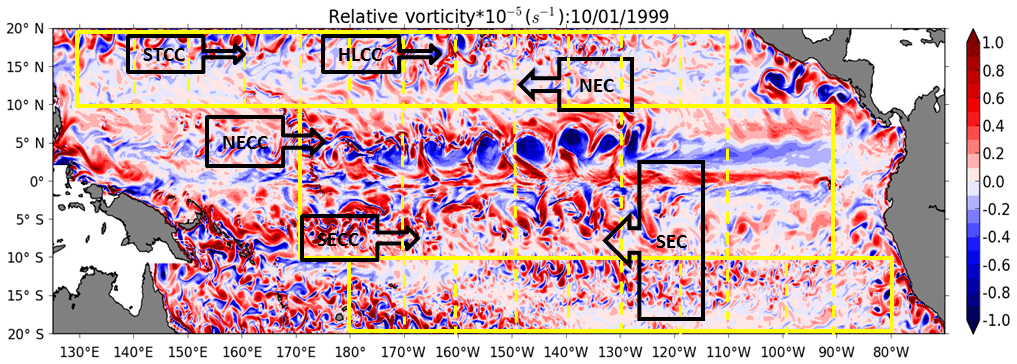
Figure 2 Snapshot of relative vorticity of the 1∕12^∘ G12d5 simulation; units are in $\mathrm{1}\times {\mathrm{10}}^{-\mathrm{5}}$ s⁻¹. The yellow lines delineate the equatorial and off-equatorial regions. The dashed lines delineate square boxes for the different regions to compute wavenumber spectra. The black arrows illustrate the main zonal tropical currents (SEC: South Equatorial Current, SECC: South Equatorial Countercurrent, NECC: North Equatorial Countercurrent, NEC: North Equatorial Current, STCC: Subtropical Countercurrent, HLCC: Hawaiian Lee Countercurrent).

The tropical Pacific is characterized by a series of strong alternate zonal currents and a large range of ocean variability, in response to the atmospheric forcing and to the intrinsic instability of the current system. The main zonal currents spanning the tropical Pacific are shown in Fig. 2: north of 10^∘ N is the westward North Equatorial Current (NEC) and at its northern edge are the eastward Subtropical Countercurrent (STCC) and the Hawaiian Lee Countercurrent (HLCC) (Kobashi and Kawamura, 2002; Sasaki and Nonaka, 2006); between 3 and 8^∘ N is the eastward North Equatorial Countercurrent (NECC); south of 3^∘ N, the westward South Equatorial Current (SEC) straddling the Equator is divided in two branches by the eastward Equatorial Undercurrent (EUC) that reaches the surface to the east. The eastward South Equatorial Countercurrent (SECC) in the southwestern Pacific is between 6 and 11^∘ S. Instabilities of these zonal currents result in meso- and submesoscale activity illustrated by a snapshot of vorticity (Fig. 2) that illustrates the description of vortices in Ubelmann and Fu (2011). It is characterized by structures with a large range of scale and strong anisotropy in the equatorial band. The largest structures (∼500 km) correspond to the non-linear tropical instability vortices (TIVs), also associated with the tropical instability waves (TIWs), and occur north of the Equator (Kennan and Flament, 2000; Lyman et al., 2007). The off-equatorial regions (10–20^∘ latitude) are characterized by smaller-scale turbulent structures in Fig. 2.

In order to investigate how these well-known tropical dynamics project into frequency or wavenumber spectra, we will analyze separately the equatorial band (10^∘ S–10^∘ N) and the off-equatorial band (10–20^∘ N and 10–20^∘ S) defined by the different boxes in Fig. 2. The model's representation of the following diagnostics will be discussed together for each zonal band: the EKE frequency spectra as a function of latitude and longitude (Fig. 3), the zonal EKE wavenumber–frequency (k−ω) spectra and meridional EKE wavenumber–frequency (l−ω) spectra (Fig. 4), and the 1-D (zonal/meridional) EKE wavenumber spectra (Fig. 5).

4.1 Equatorial region

The temporal variability of the tropical EKE signal is shown by EKE frequency spectra as a function of latitude and longitude in Fig. 3. In the equatorial band, most of the energy is concentrated within 5^∘ of the Equator (Fig. 3a). The highest EKE occurs in this band at annual to interannual scales, but there is still significant energy over all periods greater than the 10 days resolved by this model. EKE spectra averaged in latitude over 20^∘ N–20^∘ S are highly influenced by the energetic equatorial dynamics (Fig. 3b). This band includes the equatorial wave guide where waves tend to propagate zonally and are organized into a set of discrete meridional modes (Farrar, 2008). Since zonal wavenumber–frequency spectra are averaged from a number of latitudes within the equatorial band, contributions from the different modes may be seen at once (Fig. 4b). The eastward phase speed (positive wavenumber), due to fast-moving Kelvin waves at the Equator, is visible even if the strong westward propagation (negative wavenumber) just off the Equator overpowers the eastward propagation on the Equator in the averaged spectrum. We have superimposed on the zonal wavenumber–frequency spectrum the theoretical dispersion curves of the first baroclinic-Rossby waves in a resting ocean. Values of wavenumber and frequency for which the EKE power spectrum is significantly above the background follow relatively well the variance-weighted mean location of dispersion curves for long equatorial waves. Meridional wavenumber–frequency (l−ω) EKE spectra were computed over the 20^∘ N to 20^∘ S section, in different longitude bands spanning the Pacific Ocean. Figure 4d shows an example for the particularly energetic 120–150^∘ W band. Other longitude bands across the Pacific show similar spectral energy patterns but with lower energy levels. Figure 4b and d illustrate the strong anisotropy between the zonal (k, ω) and meridional (l, ω) spectra. The meridional structure of the dominant zonal equatorial waves is well known, with meridional amplitude decaying away from the Equator over ±5^∘ or 550 km. This contributes in the meridional-frequency EKE spectrum to the fairly constant decrease in spectral energy from long wavelengths down to 100–250 km wavelength, in both north and south directions (Fig. 4d).

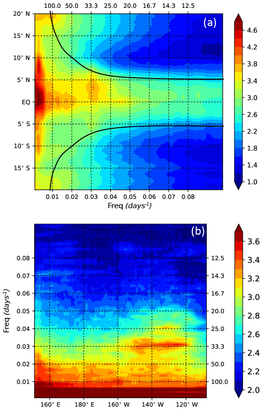
Figure 3 (a) Latitudinal distribution of the EKE frequency power spectra computed at each model grid point of the G12d5 simulation, and averaged in longitude. The black line is the critical period from Lin et al. (2008). (b) Longitudinal distribution of the EKE frequency power spectra computed at each model grid point of the G12d5 simulation, and averaged between 20^∘ S and 20^∘ N. Units are in log₁₀ of cm² s⁻² cpday⁻¹.

The ridge of westward variance (Fig. 4b) is nearly vertical, with variance mainly restricted to large wavelengths but also extending to high frequencies in relation with TIW activity. In accordance with observations (Willet et al., 2006; Lee et al., 2018), the modeled TIWs are defined by periods and zonal wavelengths in the range of 15–40 days and 800–2000 km, respectively. They have a meridional propagation with northward and southward motions roughly balanced, which is a hallmark of standing meridional modes for TIWs as seen in Lyman et al. (2005) and Farrar (2008, 2011) and earlier work (Fig. 4d). The 33-day TIW variability is triggered by baroclinic instability of the SEC-NECC system, located between 3–5^∘ N and 160–120^∘ W (Fig. 3a and b). They have an asymmetric structure across the Equator with larger energy north of the Equator than south of it in accordance with the analysis of TOPEX/Poseidon sea level data by Farrar (2008). The 20- to 25-day variability, associated with another type of TIW triggered by barotropic instability of the EUC-SEC system (Masina et al., 1999), is centered at the Equator, east of 140^∘ W (Fig. 3a and b). Centered at the Equator, from the background, there is a 60- to 80-day variability extending from 150^∘ E to 130^∘ W (Fig. 3a and b) associated with intraseasonal Kelvin waves (Cravatte et al., 2003; Kessler et al., 1995), as confirmed by eastward variance and energy centered at l=0 in the zonal and meridional-frequency spectra, respectively (Fig. 4b and d).

The model represents these tropical signals well, and for wavelengths larger than 600 km the equatorial waves are the dominant signal (Tulloch et al., 2009). For wavelengths smaller than 600 km, the variance no longer follows the Rossby wave dispersion curves, and exhibits a red noise character in wavelength, and a nearly white noise in frequency. These rapid motions with 250–600 km wavelengths occur in response to wind forcing, wave interactions, or current instability. The corresponding zonal EKE wavenumber spectrum (Fig. 5) has a steep slope that continues rising to long wavelengths with a k⁻³ relation reaching a peak at 1000 km, reflecting the zonal scales of the TIWs, before flattening to a k⁻¹ power law at larger scale. Below 70 km, EKE spectra drastically steepen as an effect of model dissipation.

4.2 Off-equatorial regions

Poleward of 10^∘, the equatorial trapped waves become insignificant, and most of the energy is concentrated at periods greater than 60 days (Fig. 3a). This corresponds to results by Fu (2004) showing a decreasing frequency range with latitude, where the maximum frequency at each latitude corresponds to the critical frequency of the first-mode baroclinic waves that varies from 60 days at 10^∘ S to 110 days at 20^∘ S (Lin et al., 2008). The zonal wavenumber–frequency spectrum strongly differs from those in the equatorial belt (Fig. 4a and c), and is closer to the midlatitude spectra (Wunsch, 2010; Wakata, 2007; Fu, 2004) with smaller energy in the south tropics than in the north as also reported by Fu (2004). The theoretical dispersion curves for midlatitude first baroclinic Rossby waves are shown for the case of meridional wavenumbers corresponding to infinite wavelengths. At low wavenumbers (i.e., long wavelengths > 600 km), the motions follow the baroclinic dispersion curves.

Although linear Rossby wave theory provides a first-order description of the EKE spectra, in both hemispheres energy extends to higher frequencies (Fig. 3a), and as the wavenumber and frequency increases, significant deviations from the baroclinic dispersion curves occur (Fig. 4a and c). Much of the energy lies approximately along a straight line called the “non-dispersive line” in wavenumber–frequency space as it implies non-dispersive motions. The wavenumber dependencies along the “non-dispersive line” could be the signature of non-linear eddies (Rhines, 1975). The westward propagation speed is estimated at ≈10 cm s⁻¹, close to the eddy propagation speed found in this latitudinal range by Fu (2009) and Chelton et al. (2007). But these regions are defined as a weakly non-linear regime (Klocker and Abernathey, 2014). In this region of mean zonal currents, the dispersion curves experience Doppler shifting by the zonal flow which makes the variability nearly non-dispersive (Farrar and Weller, 2006). So, the non-dispersive line could account for coherent vortices and more linear dynamics as Rossby waves or meandering jets propagating westward (Morten et al., 2017).

Figure 4 Zonal wavenumber–frequency EKE spectra averaged over the (a) 10–20^∘ N region, (b) 10^∘ S–10^∘ N region, and (c) 10–20^∘ S region. (d) Meridional wavenumber–frequency EKE spectra covering 20^∘ S–20^∘ N averaged over the 120–150^∘ W region. Superimposed on panels (a) and (c) are the theoretical dispersion curves for the first-mode baroclinic waves. Superimposed on panel (b) are the theoretical dispersion curves for the first three baroclinic wave modes, and the Kelvin wave mode. Units are in log₁₀ of cm² s⁻² cpday⁻¹ cpkm⁻¹.

The zonal EKE wavenumber spectra (Fig. 5) in the off-equatorial regions exhibit a standard shape with a long-wavelength plateau and a spectral break at about 300–400 km, followed by a drop in energy close to a $k^{-\mathrm{2}}/k^{-\mathrm{3}}$ relation (Stammer, 1997). These steep spectral slopes correspond to an inertial range characteristic of mesoscale turbulence (Xu and Fu, 2011). These different spectra confirm that the northern tropics are more energetic than the southern part with a mesoscale range extending to larger scale. It quantifies the more active turbulence in the Northern Hemisphere, as illustrated in Fig. 2.

4.3 Anisotropic EKE spectra

Classically, wavenumber spectra are investigated throughout an oceanic basin by dividing the basin in square boxes where spectra are calculated to take account of the regional diversity of QG turbulence properties (Xu and Fu, 2011; Sasaki and Klein, 2012; Biri et al., 2016; Dufau et al., 2016). Here, the spectra analysis of the equatorial and off-equatorial bands described above is revisited in 10^∘ × 10^∘ boxes for the off-equatorial region, and in 20^∘ × 20^∘ boxes for the equatorial region that are suited to recover the shape of the mesoscale range in the tropics (e.g., Sect. 3). Within each equatorial or off-equatorial latitude band, spectra in the different boxes are similar (not shown). Therefore, spectra are averaged over all the boxes and we present one mean spectrum representative of the square boxes for each band (equatorial and off-equatorial). In geostrophic turbulence, which is non-divergent to leading order, isotropy implies that 1-D (zonal/meridional) and 2-D azimuthally integrated wavenumber spectra (or wavenumber magnitude spectra) are identical and follow the same power law. In the tropics, there is a stronger anisotropic component of the dynamics, which will be explored in Fig. 6.

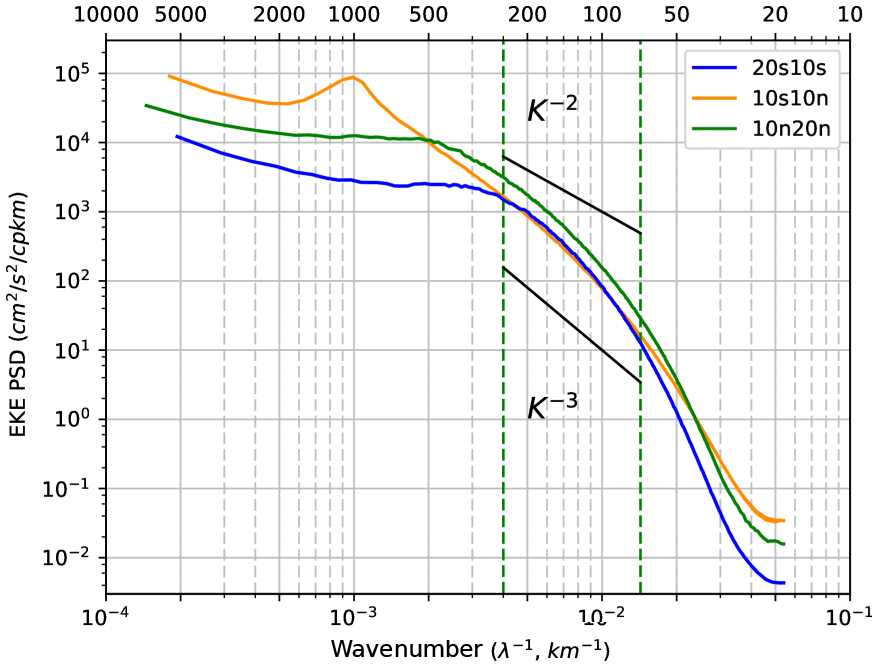
Figure 5 Zonal wavenumber EKE spectra averaged over the equatorial (orange line) and off-equatorial latitude bands (north: green; south: blue). Units are in cm⁻² s⁻² cpkm⁻¹.

When we concentrate on the 20^∘ × 20^∘ equatorial box, we are limited to wavelengths smaller than 2000 km, and the meridional EKE spectrum has a higher level of energy than the zonal one (Fig. 6b). It reflects that a given level of energy corresponds to higher zonal than meridional wavelengths. It is consistent with the widely held notion that scales of variability near the Equator tend to be larger in the zonal direction than in the meridional direction for many kinds of variability (mean currents, inertia–gravity waves, Kelvin waves, Yanai waves, TIWs). The magnitude EKE spectrum is mostly representative of the meridional one. Note that since along-track altimetry is mainly orientated in the meridional direction in the tropics, altimetric SSH measurements are particularly well suited to account for the dominant meridional variability, within the limit of the geostrophic hypothesis. Despite the anisotropy at every scale, the different EKE spectral components have a similar shape, with a continuous k⁻³ slope between 100 and 600 km wavelength. The peak of the EKE spectra corresponds to a wavelength of 1000 km. These modeling results compare relatively well with the analysis of the submesoscale dynamics associated with the TIWs by Marchesiello et al. (2011). They observe a peak of energy around 1000 km corresponding to the TIW wavelength and a linear decay of the spectrum with a slope shallower than −3. It is doubtful to define an inertial band in the equatorial region, but we can say that at wavelengths from 100 to 600 km, the EKE spectral slope of k⁻³ is consistent with a QG cascade of turbulence.

In the 10^∘ × 10^∘ off-equatorial boxes, the energy at long wavelengths is greatly reduced compared to the equatorial band. The peak of the EKE spectra corresponds to a wavelength of 300 km. Yet the zonal, meridional, and magnitude EKE spectra are similar for wavelengths up to 250 km (Fig. 6a and c). So, poleward of 10^∘, the hypothesis of isotropy seems to be relevant for scales up to 250 km even if the flow is supposed to be weakly non-linear, and sensitive to the beta effect (Klocker and Abernathey, 2014). The EKE slope over the redefined mesoscale range from 100 to 250 km is between −2 and −3, which lies between the prediction of SQG and QG turbulence.

Our modeled zonal frequency–wavenumber spectra differ strongly across the equatorial and off-equatorial regions. They show a good representation of the tropical wave and TIW/TIV dynamics. The slope of the ridge of westward variance in the zonal k−ω spectrum in Fig. 4 increases towards the Equator. As the slope becomes steeper, more power is concentrated at lower wavenumbers. The change in slope of the ridge itself is mainly related to the change in deformation radius, and expresses linear or non-linear variability propagating non-dispersively (Wortham and Wunsch, 2014). The equatorial region differs from the off-equatorial regions in having strong anisotropy with mainly zonally oriented structures (Fig. 6), higher energy at long wavelength due to the strong activity of long equatorial waves, and an overlap between geostrophic turbulence and Rossby wave timescales that produces long waves and slows down the energy cascade to eddies with scales consistent in the tropics with a generalized Rhines scale (Lr) (Theiss, 2004; Tulloch et al., 2009; Klocker et al., 2016; Eden, 2007). Moreover, our modeled spectral analysis shows the contrasts between the equatorial and off-equatorial regions for the wavenumber range where a steep slope is observed. In the weakly non-linear regime of the off-equatorial regions, we find spectral slopes of $k^{-\mathrm{2}}/k^{-\mathrm{3}}$ over a short 100–250 km wavenumber range. The equatorial dynamics are characterized by a peak of energy at 1000 km due to TIWs, and a large “mesoscale” range over 100–600 km wavelength with a k⁻³ spectral slope.

5 Modeled and altimetric SSH wavenumber spectra

5.1 Contribution from low-frequency dynamics

The SSH is a measure of the surface pressure field, an important dynamical variable, which may be balanced in the tropics by both geostrophic and ageostrophic motions. The ocean circulation is classically inferred from altimetric SSH through the geostrophic equilibrium. Here, we consider how the wavenumber spectra of geostrophic currents (EKE_g) differ from those of the total currents analyzed in Sect. 4. Close to the Equator, as f approaches zero, the geostrophic current component can still be calculated using the beta approximation, following Picaut et al. (1989). Figure 6 shows the difference between the wavenumber spectra calculated from the total EKE averaged over the upper 40 m, and from the geostrophic component of EKE estimated at the surface.

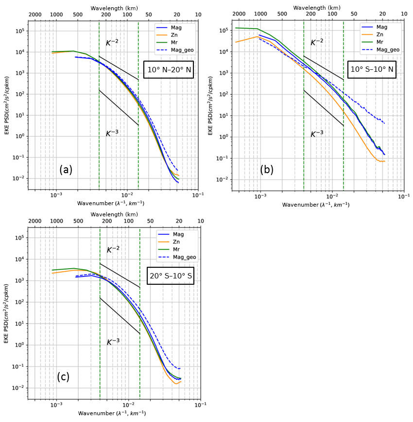
Figure 6 Zonal (orange), meridional (green), and magnitude (blue) EKE wavenumber spectra averaged over (a) 10–20^∘ N, (b) 10^∘ S–10^∘ N, and (c) 10–20^∘ S regions. The magnitude geostrophic EKE wavenumber spectrum is also shown (EKE_g, blue dashed line). The vertical green dashed lines delineate the fixed 70–250 km mesoscale range. For reference, k⁻² and k⁻³ curves are plotted (black lines). Units are in cm² s⁻² cpkm⁻¹.

In the equatorial band at scales from 300 to 1000 km, the ageostrophic EKE is more energetic, with a stronger contribution to the total EKE than the geostrophic component (Fig. 6b). In the off-equatorial bands (Fig. 6a and c), the geostrophic and total EKE spectra are similar at larger wavelengths. However, in all regions, the total EKE is steeper than the geostrophic EKE at scales from 250 km down to the 20 km resolved by the model. In midlatitude regions, Ponte et al. (2013) also noted stronger geostrophic EKE at small wavelengths (and weaker spectral slopes) compared to upper ocean EKE spectra, associated with wind-driven mixed layer dynamics. In terms of spectral slope in the equatorial region, using the geostrophic EKE rather than the total EKE tends to flatten the spectra in the 600–110 km mesoscale range, and changes the spectral slope from k⁻³ to k⁻². In the off-equatorial regions, the geostrophic EKE has a slightly flatter spectral slope between −2 and −3 in the 100–250 km band.

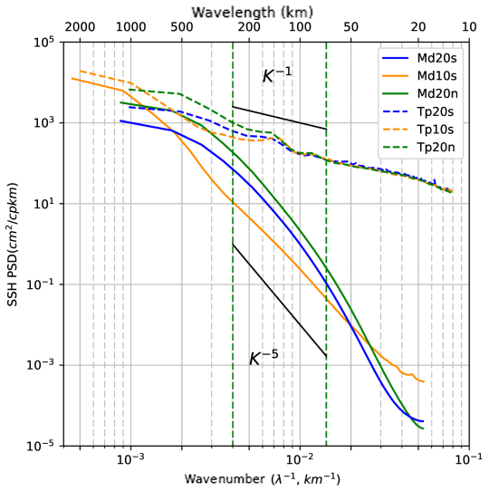
Figure 7 Meridional SSH wavenumber spectra averaged over the equatorial (orange) and off-equatorial latitude bands (north: green, south:blue) for the G12d5 simulation (line). TOPEX/Poseidon along-track altimetric SSH wavenumber spectra are averaged over the same latitude bands (dashed). Units are in cm² cpkm⁻¹.

Since the altimetric ground tracks have a more meridional orientation in the tropics, the altimetric SSH spectra should be like the model's meridional SSH spectra that are shown in Fig. 7. SSH meridional wavenumber spectra (Fig. 7) confirm that in the off-equatorial regions, the northern zone has higher spectral power over all wavelengths, as expected from the EKE_g spectra. Within the wavelength band from 100 to 250 km, both off-equatorial regions have SSH spectral slopes between k⁻⁴ and k⁻⁵ (equivalent to k⁻² and k⁻³ in EKE) similar to QG dynamics. The modeled SSH spectra show a similar anisotropy in the equatorial zone as the EKE spectra, with a more energetic meridional SSH spectrum than the zonal spectrum (not shown). It is notable that although the level of energy is higher in the equatorial region than in the off-equatorial regions, the SSH variability is lower for wavelengths smaller than 500 km. This reduced SSH variability of the G12d5 model is not in agreement with the higher small “scale” SSH levels altimetry to be discussed in the next section (Sect. 5.2). From 100 to 600 km, the SSH spectral slopes in the equatorial region are close to k⁻⁴, consistent with the k⁻² spectral slopes in EKE_g. The fixed wavelength band used by previous studies (70–250 km) can be compared to this longer wavelength band. Using the fixed wavelength band leads to a slight reduction in the low-frequency SSH spectral slope estimate but without a drastic modification. These results indicate that if the internal balanced dynamics of our 1∕12^∘ model were the main contribution to the altimetric SSH, then we would expect a k⁻⁴ (SQG) slope in the equatorial band and closer to k⁻⁵ (QG) in the off-equatorial band.

Figure 7 also shows the along-track TOPEX/Poseidon SSH spectra over the same region and period as the G12d5 simulation. The altimetric data are selected with the same segment lengths and with the same pre-processing and spectral filtering as in the model. In the equatorial and off-equatorial zones, the altimetric SSH wavenumber spectra clearly exhibit the weaker $k^{-\mathrm{2}}/k^{-\mathrm{1}}$ spectral slopes in the 70–250 km mesoscale range as described in previous studies (Xu and Fu, 2011, 2012; Zhou et al., 2015). At scales larger than our spectral slope range (600 km in the equatorial region, 200 km in the off-equatorial zones), the model–altimeter spectra have similar shapes, although the altimeter data have higher spectral power. Potentially, the high-frequency < 10-day rapid equatorial waves, with longer wavelengths not included in the model, may contribute to these differences. The spectral peaks in the altimetric data at 120–150 km wavelength are indicative of internal tides, as noted by Dufau et al. (2016), Savage et al. (2017), and others. In addition to the internal tide peaks, the general higher spectral energy in the altimetry data at wavelengths < 200 km has been proposed to be due to high-frequency internal gravity waves (e.g., Richman et al., 2012; Savage et al., 2017) but may also include altimetric errors from surface waves and instrument noise (Dibarboure et al., 2014). We will investigate the high-frequency contribution to the altimetric SSH spectra in the next section.

5.2 Contributions from high-frequency dynamics including internal tides

To investigate the contribution of the high-frequency SSH variations, we include an analysis of the meridional SSH spectra from a small region east of the Solomon Sea in the southwest Pacific. This spectral analysis is derived from the 1∕36^∘ model with high-frequency atmospheric forcing and instantaneous snapshots saved once per hour during a 3-month period, and run in the two configurations, with and without tides (see Sect. 2). The model has been validated and analyzed (Djath et al., 2014), and a companion paper will address the model with tides more in detail (Tchilibou et al., 2018). Here, we consider specifically the impact of the different high-frequency tides and non-tidal signals on the meridional SSH spectra.

The internal tide can be broken down into a coherent component that is predictable and can be separated with harmonic and modal analysis, and an incoherent component that varies over time, due to changing stratification (Zaron, 2017) or interaction with the mesoscale ocean circulation (Ponte and Klein, 2015). The coherent baroclinic (internal) tide and the barotropic tide are calculated in our study using a harmonic and modal decomposition (Nugroho, 2017) which separates the barotropic mode and nine internal tide modes, and provides a more stable energy repartition between the baroclinic and barotropic components (Florent Lyard, personal communication, 2017). Previous studies have addressed the internal tide and high-frequency components in the tropics by careful filtering of a model with tides (e.g., Richman et al., 2012; Savage et al., 2017). Aside from the issues of artifacts introduced by the tidal filtering, it is often tricky to cleanly separate the spectral contributions coming from the mesoscale ocean circulation and the incoherent component of the internal tides. The advantage of using our two-model configuration is that we can specifically calculate the high-frequency non-tidal components of the SSH spectra from the first model, and the component due to the interaction of the internal tide and the model's eddy–current turbulence with the second model.

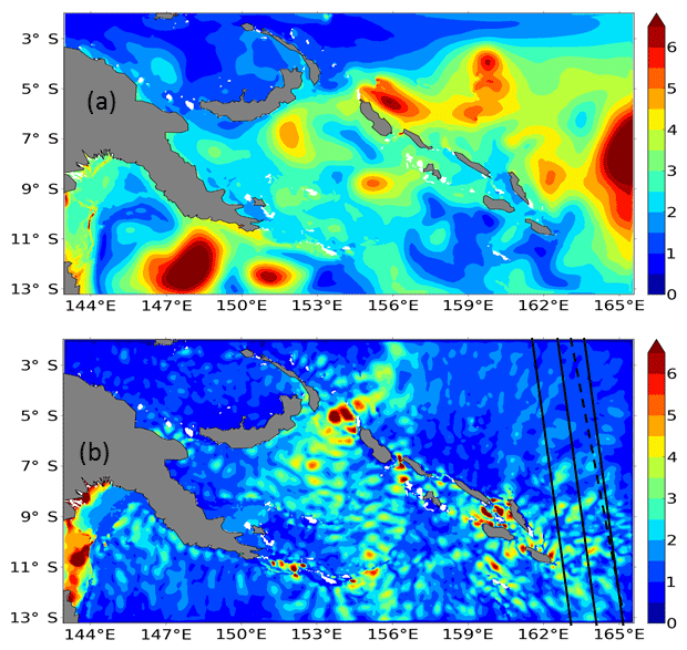
Figure 8 SSH variability of the 1∕36^∘ regional model with explicit tides (R36Th) over the 3-month simulation for (a) the mesoscale signal and (b) the internal waves and internal tides defined by a 48 h cutoff period. Units are in cm². The SARAL/ALtiKa (black line) and Jason-2 (dashed line) tracks used to compute the altimetric spectra in Fig. 9 are superimposed.

Figure 8 shows the geographical distribution of the standard deviation of SSH for the model including the tidal forcing for the low-frequency (>48 h) component of the ocean (mesoscale) dynamics and for the high-frequency component (<48 h) due mainly to internal waves and internal tides. The large mesoscale variability (up to 6 cm) east of the Solomon Sea in Fig. 8a is similar to the model without tides (not shown), and well documented as current instability from the SECC-SEC current system (Qiu and Chen, 2004). It is notable that the high-frequency variability from the model with tides in Fig. 8b is as high as the mesoscale variability, especially in the Solomon Sea, and comes mainly from the M2 baroclinic tide. We note that the M2 barotropic tide amplitude within the Solomon Sea is relatively weak (not shown), and the largest internal tide amplitudes are close to their generation sites, particularly where the barotropic tide interacts with the northern and southern Solomon Islands and the southeastern Papua New Guinea (PNG) extremities (Tchilibou et al., 2018). For the model without tides, the high-frequency variability due to the atmospherically forced internal gravity waves is very low (∼1 cm) compared to the model with tides, and shows a relatively uniform distribution (not shown).

The region used for our spectral analysis (2–13^∘ S, 163–165^∘ E; Fig. 8b) is outside the Solomon Sea with its strong regional circulation delimited by the islands and bathymetric gradients, and is more representative of the open Pacific Ocean conditions analyzed in the previous sections. The latitude band from 2 to 13^∘ S lies mostly the equatorial band defined in our previous analyses, and it is mainly representative of the SECC region (Fig. 2).

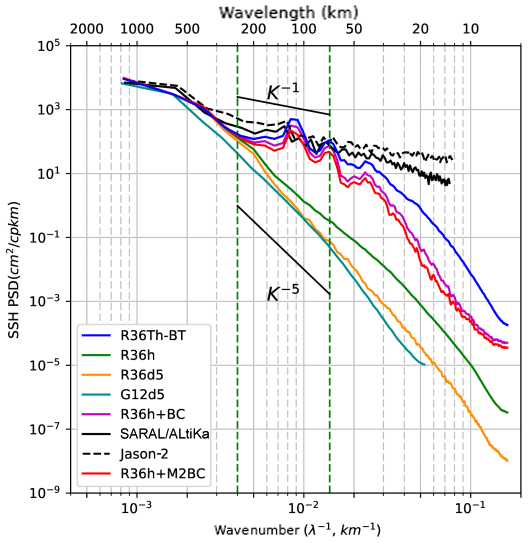
Figure 9 Meridional SSH wavenumber spectra averaged over 163–165^∘ E for the hourly outputs of the 1∕36^∘ resolution regional model without tides (R36h, green) and 5-day averaged outputs (R36d5, orange). Meridional SSH spectra of the G12d5 simulation are in cyan. SSH meridional wavenumber spectra for the hourly outputs of the 1∕36^∘ regional model with explicit tides once the barotropic tides has been removed (R36Th-BT, in blue) are shown. The spectrum of the coherent baroclinic tides has been added to the spectrum of the model without tides (R36h + BC, purple); the contribution of the only M2 coherent baroclinic tide is in red (R36h + M2BC). The difference between the blue and purple curves corresponds to the incoherent internal tides. The corresponding along-track SSH altimetric spectra for SARAL/ALtiKa (line) and Jason-2 (dashed) are in black. Units are in cm² cpkm⁻¹.

The meridional SSH spectrum from the 1∕36^∘ model run with no tides (R36h) with hourly outputs is shown in Fig. 9 (in green). The SSH from this version with no tides but averaged over 5 days is also shown (in orange), i.e., with equivalent temporal sampling to our 1∕12^∘ model analysis. The difference between these curves represents the non-tidal high-frequency component of the circulation (<10 days) due to rapid tropical waves and internal gravity waves forced by the atmospheric forcing and current–bathymetric interactions. Also shown is the spectrum calculated at the same location from our open ocean G12d5 1∕12^∘ model (in cyan) with similar spectral slope to the 5-day averaged version of our regional R36h 1∕36^∘ model, though with slightly lower energy at scales less than 70 km wavelength as expected but also in the 180 to 600 km wavelength band. So, the 1∕36^∘ model with no tides, when filtered to remove the high-frequency forcing, is quite close to the 1∕12^∘ model in this equatorial band. The main point is that the additional high-frequency dynamics in R36h increase the spectral SSH power from 300 km down to the smallest scales from 0.4 to 0.5 cm² and reduce the spectral slope calculated in the fixed 70–250 km range from k⁻⁵ with the 5-day average (in orange) to k⁻⁴ for the full model with no tides (in green).

The 1∕36^∘ model with tides (R36Th) is also shown in blue but with the barotropic tide removed. The additional meridional SSH spectral power is due both to the coherent and incoherent internal tides, with a large increase in variance up to 300 km wavelength from 0.5 cm² for R36h to 2.8 cm² for R36Th. So, the main contributors to the high wavenumber SSH spectral power are from the baroclinic tides compared to atmospherically forced high-frequency dynamics (green curve). To illustrate the respective part of coherent and incoherent baroclinic tides, the coherent baroclinic tide signature based on the nine tidal constituents summed over the first nine internal modes is calculated, and this signal is added to the model without tides (purple curve). The coherent baroclinic tides explain most of the tidal signature in the 300–30 km wavelength range, and the difference with the raw signal (blue curve) exhibits the signature of incoherent tides. The contribution of the incoherent component increases significantly at scales smaller than 30 km and explains 30 % of the SSH variance. The most energetic coherent internal tide component comes from the M2 tide, and the large increase in amplitude centered around 120–140 km wavelength corresponds to the first baroclinic mode (not shown). The other peaks around 70 km, and 40 km could be due to higher modes, and similar peaks are found in the tidal analysis of MITGCM model data by Savage et al. (2017) in the central equatorial Pacific. At the main M2 internal tide wavelengths, the incoherent internal tide has 1.6 times the SSH energy of the coherent tide, indicating that even at the main internal tide wavelengths, the incoherent internal tide is energetic.

We note that at wavelengths from 70 to 250 km used in the global altimetry spectral analysis, this 1∕36^∘ model with the full tidal and high-frequency forcing has a flat spectral slope of around k^−1.5, quite similar to the analysis of along-track spectral from Jason-2 (in dashed black) and SARAL (in solid black), in the same region but over the longer 2013–2014 period. We note that the barotropic tide has also been removed from the altimetric data, using the same global tide atlas applied at the open boundary conditions for our regional model (FES2014, Lyard et al., 2018). If we use the “mesoscale” range defined for the global model analysis in the equatorial band over 100–600 km wavelength, we still have a weak spectral slope of k⁻² for both the model with tides and altimetry. Jason-2 has a higher noise level than SARAL at scales less than 30 km wavelength (Dufau et al., 2016); the small differences in spectral energy between Jason-2 and SARAL over wavelengths from 150 to 450 km may be influenced by the different repetitive cycles of the very few tracks available (one track for Jason-2 and three tracks for SARAL/ALtiKa) between both missions and their slightly different track positions.

This regional analysis provides a number of key results. The high-frequency, high-resolution regional model confirms our open ocean 1∕12^∘ analysis. The dynamics at scales > 10 days, with no tidal forcing, give rise to SSH spectral slopes from 70 to 250 km of around k⁻⁵ in this equatorial band in accordance with the G12d5 simulation. Note that it differs from the k⁻⁴ slope typical of the equatorial region discussed above. It reflects modulation associated with low-frequency variability. This 3-month period corresponds to an El Niño event characterized by relatively low mesoscale activity in this region of the southwest Pacific (Gourdeau et al., 2014). Including the high-frequency but non-tidal forcing increases the smaller-scale energy, and flattens the SSH spectra with slopes of around k⁻⁴. This non-tidal high-frequency (<10-day) component increases the SSH spectral energy out to scales of 200 km wavelength, suggesting a dominance of rapid small-scale variability of internal gravity waves (Garrett and Munk, 1975). But the higher-frequency atmospheric forcing and ocean instabilities alone cannot explain the very flat altimetric spectral slopes in this equatorial region.

When coherent and incoherent internal tides are included, the spectral slope in the 70–250 km wavelength band becomes very close to that observed with altimetric spectra. This confirms the recent results presented by Savage et al. (2017) for a small box in the eastern tropics, and previously proposed by Richman et al. (2012) and Dufau et al. (2016). The separation of the coherent M2 internal tide demonstrates that it clearly contributes SSH energy in the 50–300 km wavelength band, but the incoherent tide, and its cascade of energy into the supertidal frequencies, is the dominant signal at scales less than 50 km. The incoherent and coherent internal tides have similar energy partitioning within the 50–300 km wavelength band.

6 Discussion and conclusion

The processes that could contribute to the flat SSH wavenumber spectral slopes observed in the tropics by satellite altimetry have been examined in the tropical Pacific. This study has used two complementary approaches to better understand how the equatorial and off-equatorial dynamics impact the SSH wavenumber spectra. In the first part of this study, we have concentrated on the low-frequency (>10-day) tropical dynamics to better understand how the complex zonal current system and dominant linear tropical waves affect the mainly meridional altimetric SSH wavenumber spectra. In the second part of the study, we have used a high-frequency, high-resolution regional modeling configuration, with and without tides, to explore the high-frequency contributions to the meridional SSH wavenumber spectra.

Our 1∕12^∘, 5-day averaged model confirms the results from previous modeling studies that at seasonal to interannual timescales the most energetic large-scale structures tend to be anisotropic and governed by linear dynamics. At intraseasonal frequencies and in the tropical “mesoscale” band at scales less than 600 km wavelength, one major question was how the cascade of energy is affected by the expected high level of anisotropy and the weak non-linear regimes. Within the “mesoscale” range, the EKE wavenumber spectra are isotropic in the off-equatorial regions between 10 and 20^∘, and it is more anisotropic in the equatorial region between 10^∘ N and 10^∘ S, with a higher level of energy for the meridional EKE spectrum than for the zonal one that reveals larger scales of variability in the zonal direction than in the meridional direction, as expected. In the off-equatorial range, EKE peaks at around 300 km wavelength, and the steep EKE decrease at smaller wavelength is characterized by spectral slopes between k⁻² and k⁻³, which lie between the regimes of SQG and QG turbulence. These weakly non-linear off-equatorial regions thus have a similar structure to the non-linear midlatitudes within the range from 100 to 250 km. In the equatorial band from 10^∘ S to 10^∘ N, the total EKE is more energetic than the off-equatorial region, and the EKE spectral slope approaches k⁻³ over a large wavenumber range, from 100 to 600 km, consistent with QG dynamics, even though there is a strong ageostrophic component here. Using the fixed wavelength (70–250 km) band to estimate “mesoscale” spectral slope leads to a slight reduction in the low-frequency spectral slope estimate but without a drastic modification. When geostrophic velocities (rather than the total surface flow) are used to calculate EKE, there is similar spectral energy in the off-equatorial regions at longer wavelengths. In the equatorial band 10^∘ N–10^∘ S, the ageostrophy is more evident with a more marked change in spectral slope based on geostrophic velocities and the beta approximation at the Equator. At large scales in the equatorial band, the ageostrophic equatorial currents are more active, related to the energetic zonal currents. In all regions, at wavelengths shorter than 200 km, the geostrophic spectra become more energetic and the small-scale ageostrophic components counteract the balanced geostrophic flow, as found at midlatitudes (Klein et al., 2008; Ponte and Klein, 2015). This gives a slightly flatter spectral slope over the 70–250 km wavelength, but the regime remains between k⁻² and k⁻³ in the off-equatorial region, approaching k⁻² (and k⁻⁴ in SSH) in the equatorial band. So, using SSH and geostrophic currents slightly flattens the EKE wavenumber spectra, but the modeled SSH wavenumber spectra maintain a steep slope that does not match the observed altimetric SSH spectra.

The choice of regional box size and filtering options also impacts on the spectra. Previous global altimetric studies have calculated along-track SSH wavenumber spectra in 10^∘ × 10^∘ boxes, and with varying segment lengths (512 km for Dufau et al., 2016; around 1000 km for Xu and Fu, 2011, Chassignet et al., 2017, etc.), and with different tapering or filtering applied (see Sect. 3). In the equatorial band where the EKE peak extends out to 600 km wavelength, it is important to have segment sizes and filtering that preserve this peak and shorter scales. The combined effects of a 10 % cosine taper and the short segment lengths lead to a much flatter altimetric SSH spectra, reaching k⁻¹ in the Dufau et al. (2016) study. We find that the double periodic spectra, the Hanning and Tukey 50 % taper filter, all give similar results in the tropics, but it is necessary to extend the box size to a minimum of 15 to 20^∘ in segment length or box size in the equatorial band. In the off-equatorial band, these filtering options with a 10^∘ segment length or box size are sufficient. Even with the preferred pre-processing for the altimetric data, and larger segment lengths in our analyses, the altimetric SSH spectra remain quite flat (k⁻² in the off-equatorial zone, k^−1.3 in the equatorial band), and do not reflect the steeper spectral slopes predicted by the model.

The regional high-resolution models with both high-frequency atmospheric and tidal forcing and high-frequency hourly outputs provide the last pieces of the puzzle. In contrast to previous results based on global ocean models with tidal forcing (Richman et al., 2012; Savage et al., 2017), this two-model configuration with and without tides has the same atmospheric and boundary forcing, which allows us to clearly separate the internal tide signals from the high-frequency dynamical component. Even though only a small region of the tropical Pacific is available for this analysis, the regional model and the global 1∕12^∘ model show similar QG spectral slopes when they are compared over the same domain and with 5-day averaged data. Using hourly data and no tides increases the SSH spectral power at scales smaller than 200 km, possibly due to internal gravity waves in the tropics (Farrar and Durland, 2012; Garrett and Munk, 1975). We note that Rocha et al. (2016) found a similar increase in their detided along-track model runs in Drake Passage but at scales less than 40 km wavelength, far below the noise level of our present altimeter constellation. In the tropics, this contribution of high-frequency non-tidal SSH signals out to 200 km wavelength will also impact today's along-track altimeter constellation, whose noise levels block ocean signals at scales less than 70 km for Jason class satellites, and 30–50 km for SARAL and Sentinel-3 SAR altimeters (Dufau et al., 2016). So, non-tidal internal gravity waves will partially contribute to the higher small-scale SSH variance and flatter spectral slopes in today's altimetric SSH data.

The regional model with tides shows the very important contribution of internal tides to the flat SSH slopes in the tropics. We have separated out the predictive part of the barotropic tide and internal tides, since open ocean barotropic tides are well corrected for in altimetric data today (Lyard et al., 2018; Stammer et al., 2014), and corrections are becoming available for the coherent part of the internal tide (Ray and Zaron, 2016). In this open ocean tropical region east of the Solomon Sea, when coherent and incoherent internal tides are included, the spectral slope in the 70–250 km wavelength band becomes very close to that observed with altimetric spectra. This confirms the recent results presented by Savage et al. (2017) for a small box in the eastern tropics, and previously proposed by Richman et al. (2012) and Dufau et al. (2016). The separation of the coherent M2 internal tide demonstrates that it clearly contributes significant SSH energy in the 50–300 km wavelength band, but around the main internal tide wavelengths, there is a strong signature of M2 incoherent internal tide. The incoherent tide, and its cascade of energy into the supertidal frequencies, is the dominant signal at scales less than 50 km. This strong incoherent internal tide is consistent with recent studies that suggest that internal tides interacting with energetic zonal jets can generate a major incoherent internal tide (Ponte and Klein, 2015), and may explain the reduction of the coherent internal tides in the equatorial band in global models (Shriver et al., 2014) and altimetric analyses (Ray and Zaron, 2016). Our model highlights that the internal tide signal is strong in this equatorial region, and the incoherent tide accounts for 35 % of the SSH spectral power in the 50–300 km wavelength band, and is not predictable.

These results have important consequences for the analyses of along-track altimetric data today, and for the future high-resolution swath missions such as SWOT. Today's constellation of satellite altimeters have their along-track data filtered to remove noise at scales less than 70 km for all missions (Dibarboure et al., 2014; Dufau et al., 2016), and these data are now being used with no internal tide correction in the global gridded altimetry maps of SSH and geostrophic currents. The imprint of these internal tides is evident in the along-track data (see Fig. 1b from Dufau et al., 2016) but is also present in the gridded maps (Richard D. Ray, personal comunication, 2017). In the future, a coherent internal tide correction may be applied to the along-track data based on Ray and Zaron (2016), to reduce some of this non-balanced signal. It is particularly important to remove the unbalanced internal wave signals from SSH before calculating geostrophic currents. But it is clear that the incoherent internal tide and internal gravity waves reach scales of 200 km in the tropics, and their signature in SSH remains a big issue for detecting balanced internal ocean currents from along-track altimetry and the future SWOT wide-swath altimeter mission. Removing this signal to detect purely balanced motions will be challenging, since filtering over 200 km removes much of the small-scale ocean dynamics of interest in the tropics. On the other hand, there will also be a great opportunity to investigate the interaction of the internal tide and ocean dynamics in the tropics in the future, with both models and fine-scale altimetric observations.

Appendix A: Model configurations used in this study

Global model at 1∕12^∘

The model used is the ORCA12.L46-MAL95 configuration of the global 1∕12^∘ OGCM developed and operated in the DRAKKAR consortium (https://www.drakkar-ocean.eu/, last access: 22 October 2018) (Lecointre et al., 2011). The numerical code is based on the oceanic component of the NEMO system (Madec, 2008). The model formulation is based on standard primitive equations. The equations are discretized on the classical isotropic Arakawa C grid using a Mercator projection. Geopotential vertical coordinates are used with 46 levels with a 6 m resolution in the upper layers and up to 250 m in the deepest regions (5750 m). The “partial step” approach is used (Adcroft et al., 1997) to allow the bottom cells thickness to be modified to fit the local bathymetry. This approach clearly improves the representation of topography effects (Barnier et al., 2006; Penduff et al., 2007). The bathymetry was built from the GEBCO1 dataset (https://www.gebco.net/, last access: 22 October 2018) for regions shallower than 200 m and from ETOPO2 (https://www.ngdc.noaa.gov/mgg/global/relief/ETOPO2/, last access: 22 October 2018) for regions deeper than 400 m (with a combination of both datasets in the 200–400 m depth range). Lateral boundary conditions for coastal tangential velocity have a strong impact on the stability of boundary currents (Verron and Blayo, 1996). Based on sensitivity experiments, a “partial-slip” condition is chosen, where the coastal vorticity is not set to 0 (“free-slip” condition) but is weaker than in the “no-slip” condition. The atmospheric forcing (both mechanical and thermodynamical) is applied to the model using the CORE bulk-formulae approach (Large and Yeager, 2004, 2009). The simulation started from rest in 1978 with initial conditions for temperature and salinity provided by the 1998 World Ocean Atlas (Levitus et al., 1998). It was spun up for 11 years using the CORE-II forcing dataset and then integrated from 1989 to 2007 using a 3-hourly ERA-Interim forcing (Dee et al., 2011).

Regional model at 1∕36^∘ with and without tides

As part of the CLIVAR/SPICE program, regional simulations of the Solomon Sea in the southwestern tropical Pacific have been performed (Ganachaud et al., 2014). The numerical model of the Solomon Sea used in this study has a 1∕36^∘ horizontal resolution and 75 vertical levels. It is based on the same oceanic component as the NEMO system presented above. This 1∕36^∘ resolution model is embedded into the global 1∕12^∘ ocean model presented above and one-way controlled using an open boundary strategy (Treguier et al., 2001). Its horizontal domain is shown in Fig. 8. The bathymetry of the high-resolution Solomon Sea model is based on the GEBCO08 dataset. Atmospheric boundary conditions, consisting in surface fluxes of momentum, heat, and freshwater, are diagnosed through classical bulk formulae (Large and Yeager, 2009). Wind and atmospheric temperature and humidity are provided from the 3-hourly ERA-Interim reanalysis (Dee et al., 2011). A first version of the regional model with 45 vertical levels has been initialized with the climatological mass field of the World Ocean Atlas (Levitus et al., 1998) and was integrated from 1989 to 2007. More technical details on this configuration may be found in Djath et al. (2014). The new version used here is distinct from the former version by the number of vertical levels (75 levels in the new version) but above all by its ability to take account realistic tidal forcing (Tchilibou et al., 2018). The model is forced at the open boundary by prescribing the first nine main tidal harmonics (M2, S2, N2, K2, K1, O1, P1, Q1, M4) as defined from the global tides atlas FES2014 (Lyard et al., 2018) through a forced gravity wave radiation condition. The model is initialized by the outputs from the ORCA 1∕12^∘ version.

Appendix B: Spectral sensitivity tests

We tested the sensitivity of our G12d5 model's SSH wavenumber spectrum to different tapering windows and the double periodic method, using different data length sizes, and in one or two dimensions. The following steps were performed for these test spectra, evaluated within 10^∘ S–10^∘ N/160–120^∘ W: the model data are extracted meridionally and zonally in fixed segment lengths of 5, 10, and 20^∘ and within a 20^∘ × 20^∘ square box; the mean and linear trend (fitted plane for two-dimensional case) were removed from each data segment or box; the filter window (Tk01, Tk05, Hann) or Dbp are applied; temporal and spatial (longitude, latitude) series spectra are calculated and averaged in Fourier space. The results are shown in Fig. B1.

Tk01 meridional spectra in the tropics are the most perturbed by the short segment lengths (Fig. B1a). In the 70–250 km range commonly used to define a global mesoscale band (delimited by the green vertical lines), the spectral slope flattens as the data segment length decreases. The 5^∘ segment spectra with a Tk01 window have a k^−1.3 slope, which explains the very shallow slope in the tropics observed by Dufau et al. (2016) who applied this short data segment size and a Tk01 window. Meridional spectra differ primarily at larger scales from 100 to 500 km, when short segment lengths are used (Fig. B1a). A comparison of the meridional spectrum using 20^∘ segments and different windows (Tk01, Tk05, Hann, and Dbp) is shown in Fig. B1b. Even with the 20^∘ segments, Tk01 is distorted. On the other hand, the Tk05, Hann, and Dbp match well, with a near-linear cascade of energy over the 30–1000 km wavelength range, and are more adapted for the tropics since they capture the main range of SSH mesoscale dynamics, particularly the spectral energy peaks around 1000 km wavelength.

Similar calculations were performed for the zonal spectra (not shown) and confirm that the Tk01 method deforms the zonal spectra and flattens the spectral slope within the 70–250 km wavelength band as the data segment size decreases. Tk05, Hann, and Dbp 20^∘ segment spectra match, although the Dbp has more noise at small scale.

We also conducted a sensitivity test in the off-equatorial region (not shown): flattening and deformation of the spectrum by Tk01 persist, but the 10^∘ segments or 10^∘ square box are long enough to capture the off-equatorial dynamics.

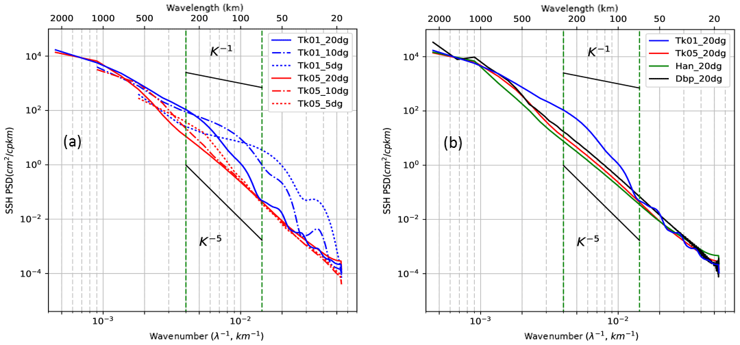
Figure B1 Sensitivity experiments for different spectral processing techniques applied to meridional SSH wavenumber spectra representative of the equatorial region. (a) SSH wavenumber spectra using a Tukey 0.1 window (blue) and a Tukey 0.5 window (red) depending on segment lengths: 5^∘ (dots), 10^∘ (dashed), and 20^∘ (line). (b) SSH wavenumber spectra using different windowing over a 20^∘ segment length: Tukey 0.1 window (Tk01, blue), Tukey 0.5 window (Tk05, red), and Hanning window (Han, green). The double periodic method (Dbp, black) is also tested. For reference, k⁻¹ and k⁻⁵ curves are plotted. Units are in cm² cpkm⁻¹.

The particular sensitivity of spectra in the tropics to the choice of spectral segment length and windowing is linked to energetic EKE and SSH signals extending out to longer wavelengths, and their spectral leakage from low to high wavenumbers. Tk01 gives the worst performance in the tropics, and the distortion of spectra is amplified for short data segments. Both the Tk05 and the Hann windowing are a good compromise for preserving much of the original signal and reducing leakage, but they need to be applied over larger segments.