Reduced cooling in the Norwegian Atlantic Slope Current: investigating mechanisms of change from 30 years of observations

The Norwegian Atlantic Current (NwAC) is a principal conduit for poleward heat and salt transport within the Atlantic Meridional Overturning Circulation (AMOC) and plays a key role of water mass transformation in the Nordic Seas. Its variability exerts a critical influence on high-latitude climate, Arctic Ocean inflows, and deep-water formation in the Nordic Seas. This study presents a comprehensive analysis of a 30-year (1993–2022) hydrographic dataset from four repeat sections across the NwAC, spanning from the southern Norwegian Sea (62.8° N) to Bjørnøya (74.5° N). Hydrographic measurements of temperature and salinity, along with derived relative geostrophic velocities, were combined with surface geostrophic currents from satellite altimetry to obtain absolute geostrophic velocities throughout the water column at each section. This allows us to robustly define the current core of the NwAC and assess its properties. The data reveal substantial variability in water properties and transport across seasonal to multiannual timescales, alongside significant warming trends. Atlantic Water (AW) cools and freshens during its journey along the Norwegian coast, but our analysis shows that north of Lofoten (69° N), the cooling has reduced by 0.11–0.13 °C per decade. We examine three potential drivers of this reduced cooling: (1) decreased air-sea heat fluxes, (2) reduced lateral heat loss due to decreasing eddy-activity, and (3) increased advection speed within the current core. We find no evidence for any changes in eddy kinetic energy, but both increased advection speed and reduced air-sea heat loss may contribute to the observed decline in cooling. Simple box model estimates suggest that while neither of the two factors can explain all variability observed in the cooling north of Lofoten, changed heat fluxes can quantitatively account for the long term trends. Our results imply a northward amplification of AW warming along the northern rim of the Atlantic Overturning Circulation.

1 Introduction

The Norwegian Atlantic Current (NwAC) is a crucial component of the Atlantic Meridional Overturning Circulation (AMOC) and serves as the primary conduit for heat and salt transport from the subtropical North Atlantic to the Arctic Ocean. The Atlantic Water (AW) within the current undergoes significant cooling and freshening as it traverses the Nordic Seas, impacting Arctic Ocean inflows, deep-water formation, and high-latitude climate (Mauritzen, 1996; Mork and Skagseth, 2010; Chafik et al., 2015; Smedsrud et al., 2022; Almeida et al., 2023). In this study, the focus lies on observed changes of the cooling of the AW within the NwAC core as it propagates northward and the processes governing it.

The NwAC consists of two main branches: the Norwegian Atlantic Slope Current (NwASC) and the Norwegian Atlantic Front Current (NwAFC, Fig. 1a). The NwASC follows the continental slope northward, exhibiting a mostly barotropic structure, while the more baroclinic NwAFC follows the Mohn Ridge in the central Nordic Seas (Orvik and Niiler, 2002; Skagseth et al., 2008; Mork and Skagseth, 2010). In a time-mean Eulerian sense, the two branches are well-defined and separated until reaching Fram Strait (e.g. Huang et al., 2023). However, recent studies based on Lagrangian tracking of drifters and simulated particles suggest some interaction between these branches, likely driven by mesoscale eddy activity in the eddy-rich Lofoten Basin region (Ypma et al., 2020; Broomé et al., 2021).

At Svinøy (off southwestern Norway ∼ 62.8° N), the volume transport of the NwAC has been estimated at 5.1 ± 0.3 Sv, whereof about 3.4 ± 0.3 Sv are associated with the NwASC, which is the focus of this study (Mork and Skagseth, 2010). There is a plethora of literature detailing the substantial spatio-temporal variability of NwASC transports along the continental slope (e.g. Mork and Skagseth, 2010; Chafik et al., 2015; Fer et al., 2020; Beszczynska-Möller et al., 2012) and the origin and propagation of thermohaline anomalies within (Furevik, 2001; Carton et al., 2011; Yashayaev and Seidov, 2015).

The current follows the continental slope northwards and bifurcates north of the Norwegian mainland into a branch flowing eastwards into the relatively shallow Barents Sea through the Barents Sea Opening (BSO, with a maximum depth of ∼ 450 m deep, Loeng, 1991; Ingvaldsen et al., 2002) and another branch continuing northwards along the continental slope, forming the West Spitsbergen Current (WSC) headed towards Fram Strait (Beszczynska-Möller et al., 2012).

Whether AW enters the BSO or continues towards Fram Strait is connected to the large scale atmospheric pattern (Lien et al., 2013; Heukamp et al., 2023). For example, wind-driven Ekman transports can cause negative sea-level anomalies around Svalbard, which in turn affect anti-cyclonic current anomalies around the archipelago, yielding enhanced flow through BSO, while reducing transport through Fram Strait (Lien et al., 2013). Similarly, the pan-Arctic atmospheric Arctic Dipole oscillation has been identified as “switchgear mechanism” between BSO and Fram Strait on multiannual time scales (Polyakov et al., 2023). On multiannual time scales, the inflow of AW into the Barents Sea has also been connected to the NAO and the Atlantic Multidecadal Oscillation, with regional hydrographic responses lagging the indices by approximately 4–5 years (Yashayaev and Seidov, 2015).

The climatic relevance for the NwASC stems not only from the transport of AW heat, but also from the substantial transformation (i.e. cooling and freshening) these waters undergo on their way towards the Arctic Ocean. For a detailed review and description of estimates of heat fluxes and (atmospheric) processes associated with the cooling, see Smedsrud et al. (2022) and the references therein.

Surface heat fluxes are generally regarded as the main drivers of cooling, as the ocean is warmer than the atmosphere for most of the year (Skagseth et al., 2020; Smedsrud et al., 2022). Over the last decades, air temperatures over the Nordic Seas have been rising faster (∼ 1 °C per decade) than sea-surface (or skin) temperatures in the region (Isaksen et al., 2022; Mayer et al., 2023), thus reducing net surface heat fluxes from the ocean to the atmosphere.

Mesoscale eddy activity also plays a critical role in lateral exchange and the heat budget of the NwASC. Eddy kinetic energy and lateral diffusivity are highest near the Lofoten Escarpment (Andersson et al., 2011), where eddies facilitate cross-slope transport. Estimates of the amount of heat that is lost from the NwASC due to westward eddy heat flux vary from roughly one-third of the NwASC’s total heat loss (Bashmachnikov et al., 2023) to claims that this may actually be the dominant mechanism of heat loss (Huang et al., 2023).

Changes of the speed of advection of AW within the NwASC may impact the time the water mass is exposed to cooling through surface heat fluxes. The investigation into changes of velocities is non-trivial because transport rates of the NwASC vary substantially along the pathway (Chafik et al., 2015). The picture is further complicated by the finding that temperature anomalies may propagate poleward at much slower speeds (by up to a factor of 10) than the observed flow of the current (Årthun et al., 2017; Broomé and Nilsson, 2018). This difference is attributed to shear dispersion, in which anomalies are mixed into slower-moving ambient waters, reducing their effective propagation speed (Broomé and Nilsson, 2018). Spiciness-based cross-correlation between Svinøy and the BSO supports this interpretation (Bosse et al., 2018). Furthermore, temperature anomalies tend to propagate more rapidly than salinity anomalies, indicating different controlling mechanisms – advection for salinity and air–sea exchange for temperature (Yashayaev and Seidov, 2015).

In this study, we use 30 years of direct ship-based measurements from four transects across the NwASC together with satellite-altimetry based estimates of surface geostrophic velocities and surface heat fluxes from reanalysis products to investigate changes in cooling of AW within the NwASC core and the associated drivers. In particular we consider three possible mechanisms impacting the cooling withing the NwASC core: (1) changes in surface heat fluxes, (2) changes in lateral heat fluxes and (3) changes in advection speeds.

2 Data & Methods

2.1 Hydrographic Data

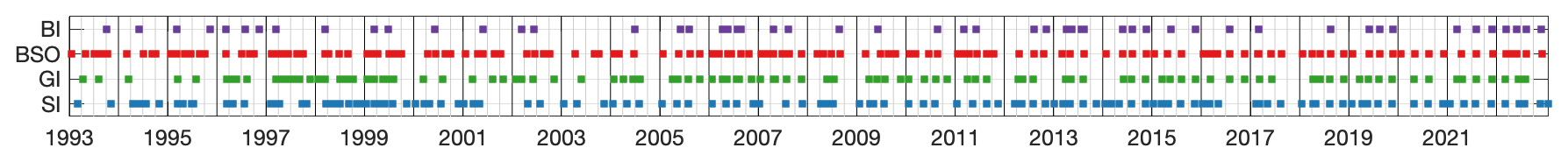
The Institute of Marine Research (IMR) has been maintaining standard hydrographic CTD (Conductivity, Temperature and Depth) sections across the Norwegian continental slope and the Barents Sea Opening (BSO) that are revisited generally several (up to six) times a year for over 50 years as part of their Norwegian and Barents Seas monitoring program. Here we use data from the most frequented sections called in order from south to north: Svinøy (SI, 17 stations), Gimsøy (GI, 16 stations), Barents Sea Opening (BSO, 20 stations) and Bjørnøya (BI, 12 stations, Fig. 1). We use data spanning the recent era with available satellite altimeter observations: 1993–2022. After automated quality control, which corrects or discards individual profiles and checks transects for completeness (detailed description in the Appendix), we are left with a total of 412 transects performed over the last 30 years. However, the distribution of these sections is irregular in time (Fig. 2). For all sections, the timing is heavily seasonally skewed, with spring and summer (MAM & JJA) accounting together for 292 transects (70 %). Svinøy, Gimsøy and BSO were frequented quite regularly over the years, amounting to 123, 105 and 131 repetitions, respectively, or average return times of 89, 102 and 83 d. Bjørnøya was only repeated 53 times over the 30 year period.

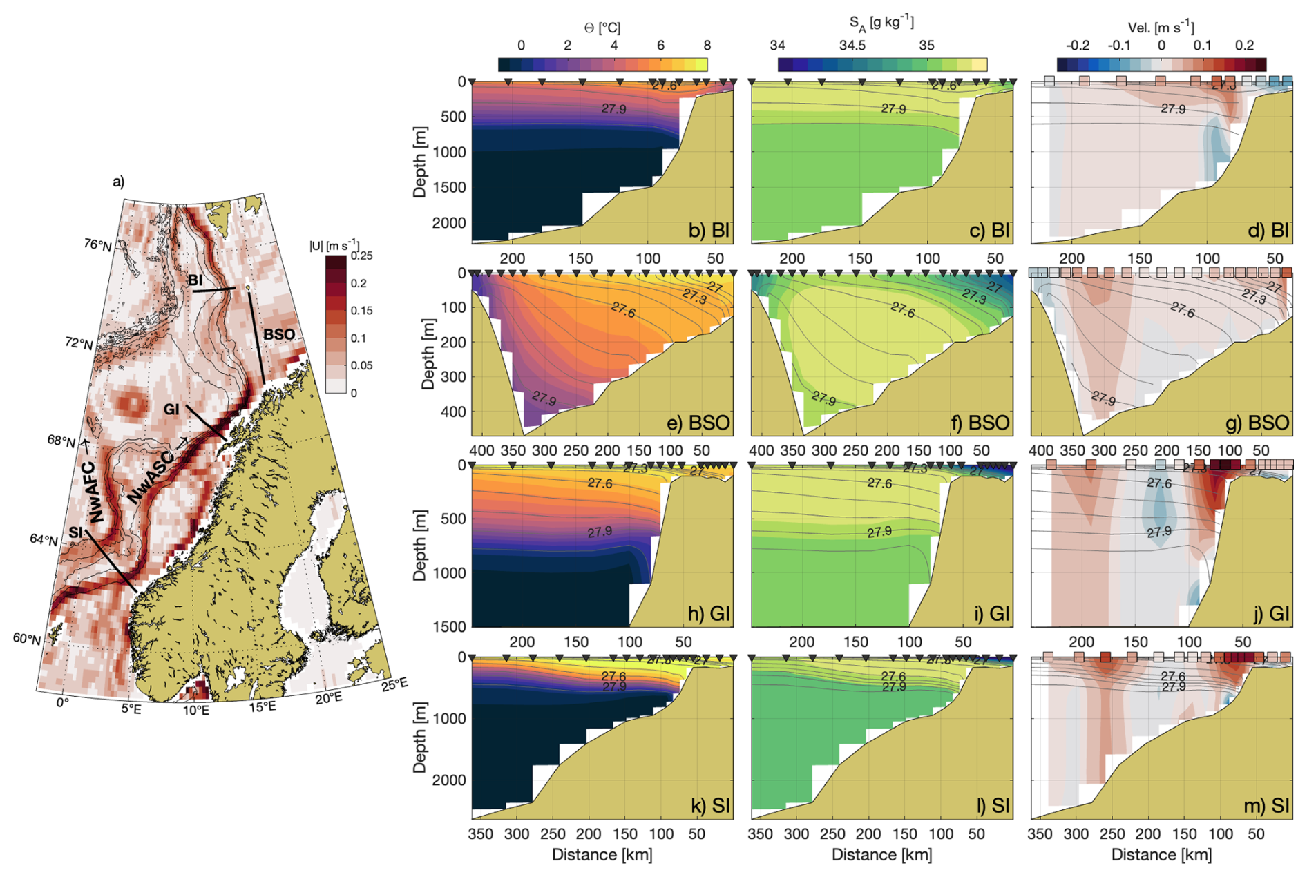
Figure 1 (a) Overview map showing the Nordic Seas and the sections indicated as black lines (SI: Svinøy, GI: Gimsøy, BSO: Barents Sea Opening, BI: Bjørnøya). Selected isobaths are given as black contour lines and color shading is satellite altimetry based surface geostrophic speed averaged over 1993–2022. Labeled in the map are the two branches of the Norwegian Atlantic Current: the Norwegian Atlantic Front Current (NwAFC) and the Norwegian Atlantic Slope Current (NwASC). (b–m) Conservative temperature (Θ), absolute salinity (S_A) and absolute geostrophic velocity (AGV) averaged over 1993–2022 for each section. Black contours are selected isopycnals and black triangles indicate locations of CTD profiles. For AGV (d, f, j, m), colored boxes at the surface indicate location and strength of average satellite altimetry based surface geostrophic velocities that are added to relative geostrophic velocity to create AGV sections.

Figure 2 Timing of each transect of the sections shown in Fig. 1.

2.1.1 Data processing

With the hydrographic transects, we obtain a snap-shot of the water column about every 3 months. This snap-shot may contain (sub-) mesoscale variability in the hydrographic properties caused for example by eddies and tides (a transect typically takes longer than one tidal cycle). For the purposes of this study, we assume that one transect should be representative of the ocean state on seasonal time scales (i.e. about 3 months). Accordingly, we endeavor to remove (sub-) mesoscale variability from the transects. Gaussian smoothing of conservative temperature (Θ, hereafter temperature) and absolute salinity (S_A, hereafter salinity) in horizontal and vertical direction often causes instability in the density stratification. Instead, we find it advantageous to effectively smooth the isopycnals in horizontal direction. This is achieved by interpolating salinity, temperature and the associated field of depths onto density coordinates. Within the density coordinates, we smooth the depths along the horizontal direction with a running mean over three stations. Since CTD stations are not always at equal distances, the smoothing distance varies. In practice this leaves us with a higher effective resolution over the continental slope, where CTD stations are close and density gradients large and effective smoothing over several Rossby-radii further offshore. The fields of temperature and salinity are then re-interpolated from the smoothed depth field to the regular depth vector and density is recalculated. This approach yields only minimal instabilities which are resolved by sorting the vertical profiles of temperature, salinity and density to ensure stability. From the smoothed, stable fields of temperature and salinity, we calculate relative geostrophic velocities (RGV) relative to the surface using the Gibbs-Seawater toolbox for Matlab (McDougall and Barker, 2011). Since RGV is based on horizontal gradients, it is calculated between pairs of profiles. In order to avoid large gaps of data at the bottom over the steep topography of the slopes, we first extend temperature and salinity of the shallower profile downwards until it reaches the depth of the deeper profile. For this, we linearly interpolate between the deepest values of the shallower profile and the deepest values of the deeper profile, so that at maximum depth the horizontal gradient is zero. If needed, the extended profile was once again re-ordered by density to maintain stable stratification (in practice only few minor inversions occurred).

Surface geostrophic velocities from satellite-based altimetry measurements are available since 1993 on a 0.125° × 0.125° grid on daily resolution (Global Ocean Gridded L 4 Sea Surface Heights And Derived Variables Reprocessed 1993 Ongoing: https://doi.org/10.48670/moi-00148, CMEMS, 2024a). Estimates of uncertainties and errors in such highly processed datasets are difficult to assess as they change over both space and time. However, using substantial parts of the same underlying satellite altimetry dataset, Mork and Skagseth (2010) found that errors in surface geostrophic velocities at Svinøy are small compared to both spatial variability along the section as well as temporal variability on seasonal to interannual time scales. To match the presumed seasonal resolution of the hydrographic transects, the satellite-derived values for surface geostrophic velocities are smoothed by running mean over a 90 d (3-month) period before interpolating them to the locations of RGV data points (in-between original CTD stations). Adding the satellite-derived surface geostrophic velocities to the field of RGV yields a field of absolute geostrophic velocity (AGV) for each transect. We note that in the time-averaged AGV sections, there appears to be a weak southward flow underneath the NwASC current core at Svinøy, Gimsøy and Bjørnøya (Fig. 1d, j, m). Due to the slope of the isopycnals, relative geostrophic currents are all southward in these sections, typically increasingly so with depth. The northward flow only comes to be when adding the satellite-derived surface geostrophic currents. It is thus possible that these southward flows underneath the current core may be artifacts, either due to slightly too steep isopycnal gradients at the slope, or too weak surface geostrophic northward currents (owing to the spatial averaging involved in the satellite product processing). Since overall transport estimates (presented in Sect. 3.1) are within the ranges reported in literature, we do not consider this to be problematic for our analyses.

2.1.2 Defining the AW current core and creating time series

Obtaining meaningful and comparable time series of properties from different sections of varying spatial coverage of the NwASC can be non-trivial. In this study, we focus on the properties of the NwASC core, which we can compare between sections. We first bound the area for each section based on 30-year mean properties as follows:

• Contains Atlantic Water (AW), defined via S_A≥35.16 g kg⁻¹, following common definitions (Mork and Skagseth, 2010; Ingvaldsen, 2005; Loeng, 1991).

• Has an upper boundary of 50 m below sea surface (to exclude large parts of the seasonally varying surface layer).

• Is located shore-ward of the 1500 m isobath (SI) or 2500 m isobath (GI), to avoid the NwAFC and large scale recirculation, respectively.

Figure 3 Sections of average AGV (as Fig. 1d, g, j, m, but zoomed in on the continental slope), with selected isotherms as colored contours. Areas (shading) and actual data points (markers) comprising the core and non-core as defined in Sect. 2.1.2 are shown in cyan and gray, respectively.

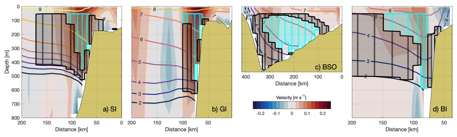
Each data point within these areas is associated with a transport, calculated by multiplying AGV at the respective point with the area it represents, whereby the area is assumed to be rectangular, bounded by the mid-distance to adjacent points. This approach does not account for topography “cutting” through the area of individual cells at the boundary and thus represents a slight overestimate. Cumulative summation of the transports within the area yields total AW transport through the section. At Svinøy, Gimsøy and Bjørnøya, the NwASC core is defined to consist of the data points – sorted by decreasing AGV – needed to account for 50 % of the total mean transport through the respective section. This yields an NwASC core defined by the strongest currents within the AW layer (Fig. 3a, b, d). At BSO, the situation is different; the topography is a lot shallower and there is no pronounced mean boundary current (Fig. 1g). Thus, the strongest mean currents do not represent the core of the AW. Instead, we use salinity so that the core is defined to consist of the data points – sorted by decreasing salinity – needed to account for 50 % of the maximum mean transport through the section. This yields a core consisting of the highest salinity waters, thus ensuring that it is indeed waters from the NwASC core (Fig. 3c). This approach excludes fresher coastal current waters as well as waters originating from the NwAFC that may have recirculated towards the BSO (Broomé et al., 2021), but most likely would have freshened (and cooled) substantially en route. Core (and non-core) properties are then averaged within the respective core (or non-core) area for each transect at each section. This core definition is based on average properties and thus static over time. Experiments with dynamic definition of core area for each individual transect yielded some variability, but no substantial (nor significant) trends in area or location of the core (not shown). We further note that for the scope of this study, the properties of the core are qualitatively insensitive to the choice of percentage of max transport (tested in a range from 50 %–70 %).

The spatial extent, as well as the shape of the core and non-core varies substantially between sections (Fig. 3). At Svinøy, the core is wedge-shaped, centered roughly above the 600 m isobath and reaching a maximum depth of 460 m (Fig. 3a). At 50 m it has a lateral extent of about 50 km, comprising 4 CTD casts. Horizontally, the non-core area is limited by the 1500 m isobath, which is about 150 km offshore and vertically reaching down to 530 m where it is bound by salinity. At Gimsøy, the exceedingly steep topography yields a vertically more stretched core and non-core, reaching down to 530 and 630 m respectively while each only extending about 50 km horizontally due to the defined boundary at 2500 m isobath (Fig. 3b). In the Barents Sea, where the core is defined via salinity, it makes up large parts of the water column over the shallow southern slope down to about 350 m water depth (Fig. 3c). The non-core area surrounds the core, with the largest area located over the deep trench and the steep northern slope of the BSO. The core and non-core areas at Bjørnøya strongly resemble those at Svinøy, albeit reaching slightly deeper (about 580 m, Fig. 3d).

To make the time series of the individual sections comparable, we interpolate them onto a common time vector with 3-month time resolution. While the time resolution corresponds roughly to the average return time for the Svinøy, Gimsøy and BSO sections, this does not take into account the seasonal bias of the actual transects (Fig. 2). For Bjørnøya, the 3 month interpolation corresponds on average to an oversampling and care has to be taken interpreting results based on this interpolation. For some analyses, de-seasoning is necessary, which is performed by 12-month moving averaging of the 3-month interpolated time series.

2.1.3 Correlations

Due to the substantial seasonality of some properties (e.g. temperature), correlations are done using the annually smoothed and de-trended 3-month interpolated time series (except when stated otherwise). A side effect of the smoothing is that neighboring points are not independent from each-other which has consequences for the calculation of the correlation coefficient. To account for the auto-regression, significance intervals for all correlation coefficients presented in this study are calculated using the effective degrees of freedom via the modified Chelton method presented in Pyper and Peterman (1998).

2.1.4 Cross-correlations

To investigate advection times of anomalies between sections, we use 12-month smoothed salinity time series and calculate cross-correlations in various windows (ranging from 5 to 15 years in size), sliding at at increments of $\mathrm{1}/\mathrm{4}$ window length. As the window slides over the time series, the lag of the highest cross-correlation within each window is calculated. Only results with satisfactory data coverage (at least 50 % of expected quarterly data points within any window), significant correlation coefficients (at 95 % confidence) and sensible lags (between 0 and 24 months) were taken into account. Due to sparse sampling, Bjørnøya was excluded from this analysis.

2.2 Heat fluxes

Heat fluxes and other meteorological parameters (2 m temperature, 10 m wind and sea-surface temperature) in the study domain are obtained from ERA5 reanalysis on a 0.25° × 0.25° grid and provided as monthly averages (Hersbach et al., 2020). We define positive heat fluxes to be directed upwards from the ocean to the atmosphere. Uncertainties associated with heat fluxes can be large, but independent estimates from energy budget closures showed that at leas the direction of observed trends is robust over the Nordic Seas (Mayer et al., 2023).

2.3 Box model estimates

The impact surface heat fluxes have on ocean temperatures, can be estimated using a simple box model. In particular, we solve the following equation

$$\begin{array}{}\text{(1)}& \mathrm{\Delta }T=H_{\mathrm{f}}{B}_{\mathrm{surf}}t/\left({\mathit{\rho }}_{\mathrm{w}}{B}_{\mathrm{vol}}c{p}_{\mathrm{w}}\right)\end{array}$$

with the temperature change ΔT equaling the surface heat fluxes H_f (obtained from ERA5), acting over the duration of the (advection) time t on the surface of the box B_surf, impacting a volume of water defined by the density of sea water ρ_w=1027.6 kg m⁻³ (corresponding to the average NwASC core water density at Gimsøy), the volume of the box B_vol, and the specific heat of water $c{p}_{\mathrm{w}}=\mathrm{3.9919}\times {\mathrm{10}}^{\mathrm{3}}$ J kg⁻¹ K⁻¹. The dimension of the box is given by the respective length of the pathway between two sections (about 750 km for the path between Gimsøy and Bjørnøya), the width of the box set to 50 km (based of Fig. 3 and Huang et al., 2023). This yields a surface of the box $B_{\mathrm{surf}}=\mathrm{750}\times {\mathrm{10}}^{\mathrm{3}}$ m × 50 × 10³ m = 3.75×10¹⁰ m². The area of the cross-section is set to 10 km², which is representative of the core areas at Svinøy, Gimsøy and Bjørnøya (about 11, 8 and 17 km², respectively). This yields a depth of the box of 200 m, with the total volume of the box $B_{\mathrm{vol}}=B_{\mathrm{surf}}\times \mathrm{200}$ m $=\mathrm{7.5}\times {\mathrm{10}}^{\mathrm{12}}$ m³. Due to the absence of any vertical mixing parameterization in the box model, absolute values obtained for ΔT will be heavily biased, but anomalies will be interpretable under the assumption of approximately linear scaling of mixing with respect to surface heat fluxes.

3 Results

3.1 Time-average properties of the NwASC

In a time-mean sense, the Θ-S_A properties of both core and non-core areas show a systematic cooling and freshening from south to north (Fig. 4). The core always contains warmer and more saline waters than the non-core, which may be readily explained by lateral mixing with surrounding water masses and increased vertical heat fluxes due to the slower, possibly more meandrous propagation of water in the non-core areas. In the BSO, the core is by definition more saline than the non-core, but it is also substantially warmer than the Bjørnøya core. This may be partly due to a somewhat shorter pathway from Gimsøy to BSO compared to Gimsøy to Bjørnøya, and partly due to extensive mixing between the water in southern part of BSO core and non-core areas and the warm and fresh coastal current, whose Θ-S_A properties show clear mixing-lines with the core and non-core Θ-S_A properties (not shown).

Average transport estimates are by definition identical for core and non-core areas of each section. The combined core and non-core transport is 2.60, 2.29  1.51 and 2.17 Sv for the Svinøy, Gimsøy, BSO and Bjørnøya sections, respectively. This is within the range of values presented in the literature for various periods (Mork and Skagseth, 2010; Fer et al., 2020; Ingvaldsen et al., 2004; Beszczynska-Möller et al., 2012).

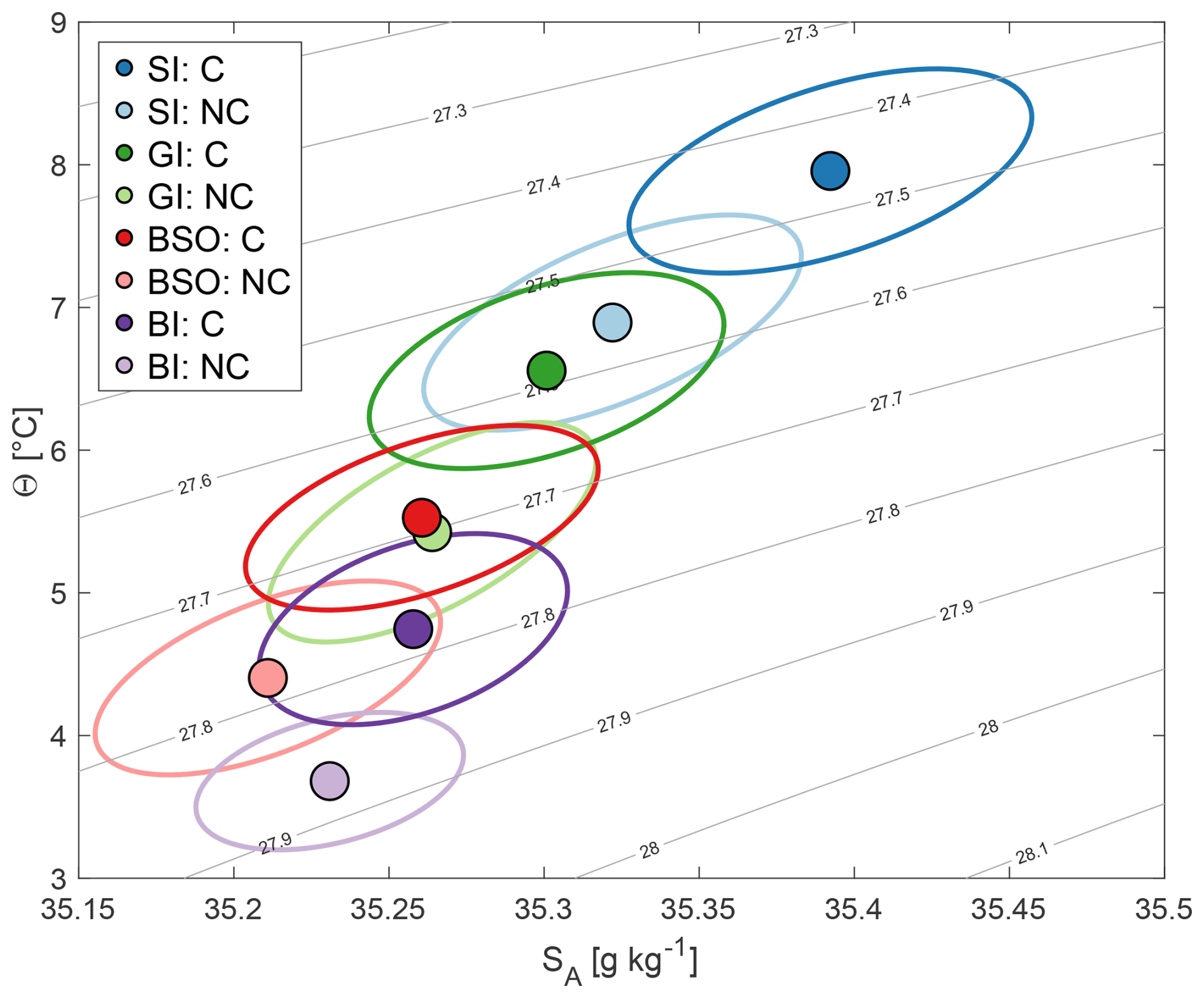
Figure 4 Θ-S_A diagram of time-average properties averaged within the core (C) and non-core (NC) of each section. Ellipses indicate 50 % variance.

3.2 Temporal variability of NwASC properties

Time series of temperature, salinity and transport exhibit substantial interannual variability throughout the 30-year time period (Fig. 5). Especially notable are the significant trends of temperature at all sections for both core and non-core area averages (bold font in the legend, Fig. 5a–d). For salinity, there are no significant trends anywhere, but the multiannual variability is most pronounced with an increase of over 0.1 g kg⁻¹ during 1995–2010 at all sections, followed by a near-synchronous more rapid decrease after 2015 (Fig. 5e–h). Interestingly, this change of salinity does not appear to have substantially impacted density, which exhibits variability and significant negative trends in accordance with changes in temperature (not shown). While showing substantial interannual variability, there does not appear to be any structured multiannual variability in RGV (not shown) or transports, nor are there any significant trends (Fig. 5i–l). All analyses and discussions in the remainder of this manuscript are based on the core properties only.

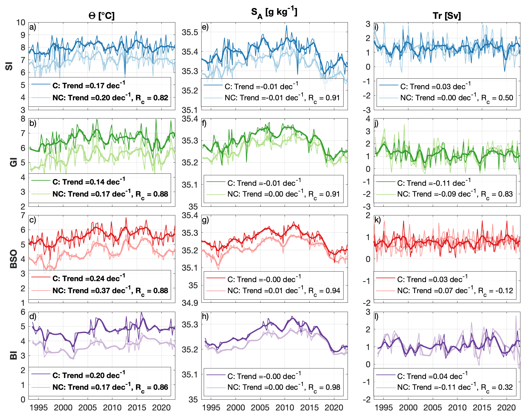
Figure 5 Time series of core (solid colors) and non-core (lighter colors) properties for each section, both in original time resolution (thin lines) and on annually smoothed 3-month interpolated time vector (thick lines). Legends in each panel show the linear trend (calculated from the original, un-interpolated time series) and correlation to the core time series. Bold font in the legend indicates trends that are different from zero at 95 % confidence.

3.3 Cooling of the NwASC core north of Gimsøy: long term trends, variability and potential drivers

In a steady regime of cooling and freshening, the difference of temperature and salinity between sections may be constant regardless of overall trends in the properties. Between Svinøy and Gimsøy, variability of temperature differences is about 1 °C and the trend of −0.03 °C per decade is not significantly different from zero at the 95 % confidence interval (Table 1). Going further north, differences between both Svinøy and BSO as well as between Svinøy and Bjørnøya exhibit significant decreasing trends of −0.13 °C per decade each. The absence of a trend between Svinøy and Gimsøy suggests that most of these trends manifest north of Gimsøy. Indeed, trends in the temperature difference between Gimsøy and BSO as well as Gimsøy and Bjørnøya are almost identical to those relative to Svinøy, with −0.11 and −0.13 °C per decade, respectively (Table 1). There is no significant trend in temperature difference between BSO and Bjørnøya (Table 1). Trends of salinity differences are also negative throughout, but only significant for all differences involving Bjørnøya. Amplitudes are small (≤ 0.016 g kg⁻¹ per decade, Table 1). In summary, these results indicate reduced cooling of AW between Gimsøy and BSO/Bjørnøya and thus point towards a change of heat loss mechanisms.

Interannual variability of cooling within the NwASC north of Gimsøy can be estimated by calculating the temperature difference (ΔΘ) between Gimsøy and BSO (Bjørnøya is excluded from this analysis due to sparse sampling) using plausible advection times of 3–12 months to capture the range associated with advection speed uncertainty. To facilitate comparisons with further analyses, anomalies are shown and a smoothing of 3 years is applied to emphasize longer term variability (Fig. 6, blue line and shading). The largest ΔΘ anomalies are observed around 1997 and 2003. After 2005, amplitudes of ΔΘ anomalies decline and become more negative, reflecting the overall reduction of cooling shown in Table 1. The most negative ΔΘ anomalies are found between 2017 and 2020 and appear to be mostly due to two individual strong negative temperature anomalies at Gimsøy, that are not represented at any other section (Fig. 5a–d). In the following, we investigate possible drivers behind the reduced cooling north of Gimsøy and its variability.

Table 1 Trends of temperature differences calculated pairwise between all sections for core temperatures. As before, bold font indicates trends that are significantly different from 0 at 95 % confidence.

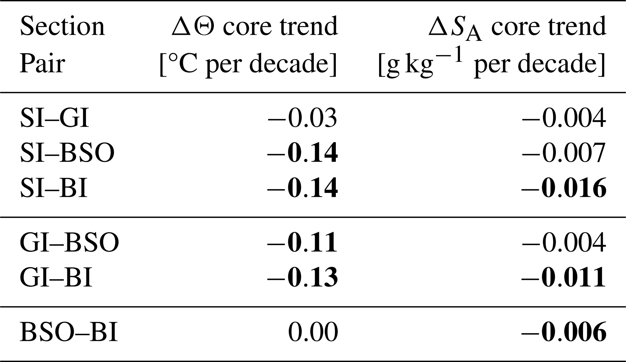
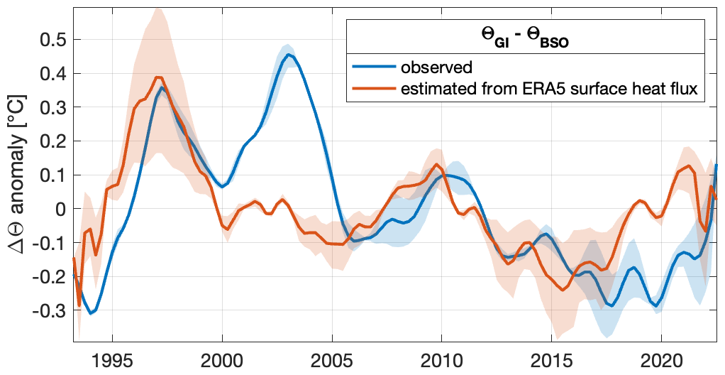
Figure 6 3-year smoothed time series of ΔΘ core anomalies between Gimsøy and BSO. Blue are observations, red are estimated from ERA5 heat fluxes using a simple box model. Shading is the envelope of results using different advection times, ranging between 3 and 12 months (cf. Fig. 8b), solid lines are the average of the envelope.

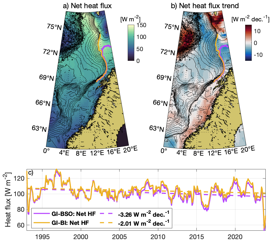
Figure 7 (a) Net heat flux averaged over 1993–2022. (b) Linear trend of net heat flux. (c) Time series and linear trends of the net heat flux averaged over the line segment along the 400 m isobath between Gimsøy and BSO (purple) and for the line segment along the 500 m isobath between Gimsøy and Bjørnøya (yellow). As before, significant linear trends are written in bold font.

3.3.1 Reduced cooling through the surface

Surface heat fluxes account for the largest loss of heat from the ocean in the Nordic Seas, with 30-year averages reaching 60 W m⁻² over the Nordic Seas (full domain of Fig. 7a), and exceeding 100 W m⁻² in the vicinity of BSO and Bjørnøya (Fig. 7a). Over the last 30 years, surface heat fluxes have decreased substantially, specifically in the region between Gimsøy and BSO/Bjørnøya (Fig. 7b). In particular along the pathway of the AW entering the BSO following the 400 m isobath, net heat flux from the ocean to the atmosphere has reduced by 3.26 W m⁻² per decade, or about 3 % per decade (Fig. 7c). Notably all components contributing to net heat flux (sensible heat flux, latent heat flux, shortwave radiation and long wave radiation) show significant trends with shortwave radiation being the only component with a positive trend (0.45 W m⁻² per decade) and sensible heat flux accounting for the vast majority of the net decrease with −2.58 W m⁻² per decade (not shown). When following the pathway of NwASC along the 500 m isobath between Gimsøy and Bjørnøya, the negative net heat loss trend is somewhat smaller with −2.01 W m⁻² per decade and sensible heat flux is the only component with a significant trend (−2.15 W m⁻² per decade). The reduced net heat flux from the ocean to the atmosphere causes less cooling and may thus contribute to the decrease in core temperature difference between Gimsøy and BSO/Bjørnøya (Table 1). Simple box-model budget calculations (Sect. 2.3) indicate, that in order to increase the temperature of a volume of water set to represent the NwASC core between Gimsøy and Bjørnøya by 0.13 °C, corresponding to the observed reduced cooling trend in Table 1, heat fluxes of about 3.3 W m⁻² suffice, assuming an incubation time (i.e. advection time) of 12 months. These estimates indicate that surface heat flux may be the dominant driver for changes in the cooling along the NwASC.

To estimate in how far the observed variability of cooling may be attributed to variability of surface heat fluxes, the afore mentioned simple box model (Sect. 2.3) is forced by realistic 3-year-smoothed ERA5 heat fluxes. It is important to note, that in the absence of a realistic mixing parameterization, absolute values of the box model results will be biased and results are only meaningful as anomalies. Since advection time act as scaling factor in the model (Eq. 1), the anomalies calculated using different advection times (3, 6, 9 and 12 months) all have different base-lines. Box model estimates closely follow the observed ΔΘ anomaly peak between 1995 and 2000, as well as variability from 2005 to 2017 (Fig. 6, red line and shading). This suggests that surface heat flux variability can explain much of the cooling variability in those periods. Larger discrepancies arise during 2000–2005, when observed anomalies exceed model estimates by ∼ 0.4 °C, and during 2017–2021 when model estimates exceed observations by ∼ 0.2 °C. In these periods, surface heat loss changes alone cannot account for the observed cooling variability.

3.3.2 Reduced cooling by reduced lateral heat flux

It has been estimated that eddy-driven lateral heat transport accounts for about one third of heat loss from the NwASC (Bashmachnikov et al., 2023). However, lateral heat fluxes (e.g. via baroclinic and/or barotropic energy conversion) are difficult to directly observe and require dedicated observational efforts. The only long term moored observations in the region are located at the Svinøy section over the 500 m isobath. There, moored current meters have been operational continuously over the whole period of interest in this study (1993–2022). EKE is calculated at 100 m water depth using daily bin-averaged velocity fluctuations as deviations from 30 d averaged means and then interpolated on the common 3-month time vector. The average EKE is 0.0087 m² s⁻² and shows a slightly negative linear trend over 30 years (−6.4327 $\times {\mathrm{10}}^{-\mathrm{4}}$ m² s⁻² decade⁻¹) that is not significant (p=0.102). Decreased (or increased) lateral heat fluxes, could be expected to increase (or decrease) the lateral temperature gradient. This is not observed at any section crossing the NwASC. The verdict on whether the lateral heat flux has changed in the area thus remains inconclusive.

3.3.3 Increased advection speed leaves less time to cool

Time series of RGV and transports do not show any significant trends at any section (Fig. 5). An independent measure of advection along the NwASC lies in the tracing of anomalies as they propagate through the sections. Because of its small influence on density in the domain, salinity acts largely as a tracer and is thus best suited to investigate advection speed of signals, and shifts in these, along the continental slope. Cross-correlation lags of salinity anomalies for the segment Gimsøy to BSO (Sect. 2.1.4) are plotted centered within their respective window (colored dots) and two-year bin-averaged lags are shown as black lines in Fig. 8. While the effective smoothing is uneven and ranges between 5 and 15 years, depending on the respective window, tests showed good temporal fidelity of the analysis. Reassuringly, the sum of the mean lags calculated in the segments Svinøy to Gimsøy and Gimsøy to BSO corresponds well with the estimate of lags between Svinøy and BSO (i.e. they agree within the 3-month temporal resolution, not shown). The estimates show substantial variability of advection times, ranging between 0 and 12 months. Despite an absence of reliable results before 2000, there is a clear and robust pattern visible. In particular, on the segment from Gimsøy and BSO (Fig. 8), lags of 9–12 months dominate the time interval from 2002 to 2011. After that there is a continuous and robust reduction in lags to 0–3 months. Such drastic variability is not represented in either transports (Fig. 5i–l), nor satellite-derived surface geostrophic currents (not shown). However, it is known that advection speed of anomalies can differ substantially from observed current speeds due to internal processes such as velocity shear (Broomé and Nilsson, 2018). To investigate this, we estimate vertical shear for each time step by creating a mean velocity profile from horizontally averaging AGV within the core and integrating the vertical shear of this profile. Time series of total vertical shear at the Gimsøy section shows variability similar to the cross-correlation analysis (Fig. 8 purple line), with decreasing lags in recent years coinciding with reduced vertical shear observed at Gimsøy (note that total vertical shear is generally negative here, such that a reduction manifests in a rising curve).

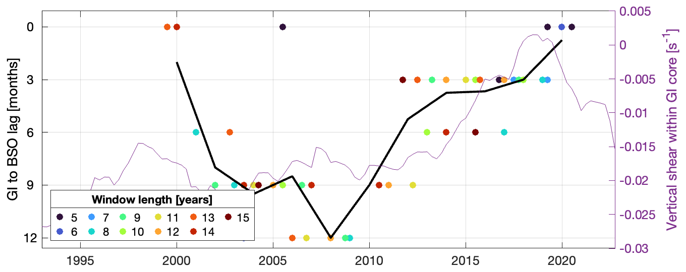
Figure 8 Lags of maximum cross-correlation of 12-month smoothed S_A between Gimsøy and BSO within various windows ranging from 5–15 years (colors of dots), sliding at increments of $\mathrm{1}/\mathrm{4}$ window length. Shown are only results with significant correlation coefficients (p≤0.05), positive lags (between 0 and 24 months), and where both time series have at least 50 % of the expected (quarterly) data points in any given window. The black line represents bin-averaged lags in two-year bins. The purple line shows time series of total vertical shear within the core at Gimsøy, smoothed with a 5-year running mean.

4 Discussion

This study presents robust observational evidence of a long-term reduction in the cooling of AW in the NwASC core north of Gimsøy, particularly between the Gimsøy and the BSO and Bjørnøya sections. The trend in core temperature differences between these sections exceeds −0.11 °C per decade (Table 1), with the strongest signal observed in the Gimsøy–Bjørnøya segment. Our results indicate that both reduced surface heat fluxes and faster advection speeds likely contribute to the observed trends, whereas lateral heat loss does not appear to have undergone any systematic change. Simple box model calculations further point towards time-varying interplay between drivers determining heat loss along the NwASC path. Below, we discuss our key results in the context of existing literature.

4.1 Reduced surface heat loss as a primary driver of change

Net surface heat loss along the NwASC pathway between Gimsøy and BSO/Bjørnøya has significantly declined by ∼ 3 % per decade over the past three decades, with trends exceeding −2 W m⁻² per decade along the 400 m isobath (Fig. 7). This reduction stems mostly from the northeastern part of the Lofoten Basin and is dominated by decreasing sensible heat fluxes. Drivers behind this trend are reduced air-sea temperature gradients due to the former warming faster than the latter. Mayer et al. (2023) suggest that his may be attributed to more southeasterly winds, ultimately related to a strengthening of the Icelandic low that advect warmer air masses from lower latitudes. Surface heat fluxes are known to be a key driver of heat content variability in the region (e.g. Mork et al., 2019), but timescales and amplitudes of associated anomalies are under debate (Carton et al., 2011; Yashayaev and Seidov, 2015). Furthermore, heat fluxes can be seen as both cause and consequence of a changing ocean heat: if the ocean warms relative to the atmosphere, heat fluxes increase, indicating increased cooling (Asbjørnsen et al., 2020). In terms of variability, our box model analysis using ERA5 heat fluxes indicate that surface fluxes reproduce observed temperature difference anomalies between Gimsøy and BSO for several time periods (Fig. 6), particularly from 1995–2000 and 2005–2015. At the same time, discrepancies between modeled and observed anomalies (e.g., 2000–2005 and post-2017) point towards other drivers of variability. Using the box model, we can estimate the relative changes in advection time that would be needed to account for the observed temperature difference anomalies. In particular, in order to achieve the ∼ 0.45 °C anomaly observed in 2003 with the realistic ERA5 surface heat fluxes, advection speeds need to reduce by about 50 % relative to the mean advection speed (this coincides with low observed transports in 2003 at Gimsøy, Fig. 5j). Conversely, to account for the $\sim -$0.3 °C anomaly observed in 2017, an acceleration of ∼30 % relative to the mean advection speed is required. This is in qualitative agreement with the changes in advection speed we deduce from the advection of salinity anomalies for the Gimsøy-BSO segment (Fig. 8). Apart from changes of advection speed, changes in surface area would also influence the impact of surface heat fluxes. Using hydrographic data spanning both the NwASC and NwAFC north of Svinøy, Blindheim et al. (2000) found a broadening (narrowing) of the AW expanse in response to decreased (increased) wind forcing that has been observed to correlate with NAO on interannual time scales. Experiments with varying AW core at Gimsøy (following the same definition as described in Sect. 2.1.2, but estimated at every time step instead of using the mean fields) showed indeed some (intermittent) anti-correlation of core width with NAO. However, we found no systematic pattern of core width changes in the periods of marked discrepancies between modeled and observed anomalies (e.g., 2000–2005 and post-2017). In these cases, other processes may play a role, such as varying baroclinic conversion at the Lofoten Escarpment (Fer et al., 2020) or general periods of discontinuity (Chafik et al., 2015) may also be the reason that anomalous upstream signals at Gimsøy are not advected further north (see Fig. 5a–d).

4.2 Increased advection speed

While transports derived from geostrophic velocities from hydrographic transects and satellite-derived surface currents do not display significant long-term trends (Fig. 5i–l), independent evidence comes from salinity anomaly propagation. Cross-correlation analysis (Fig. 8) reveals a substantial decrease in lag times between Gimsøy and BSO, where the average lag decreases from approximately 9–12 months in the early 2000s to 3–6 months after 2015. Although salinity anomalies do not necessarily travel at the same speed as temperature (or heat) anomalies (Yashayaev and Seidov, 2015), this implies an acceleration of advection speed, reducing its residence time and thereby limiting heat loss to the atmosphere. The notion that advection speed changes while geostrophic transports (Fig. 5i–l) and satellite-derived surface currents (not shown) are steady may appear to be inconsistent, but it is well known that advection speeds can be up to 10 times lower than observed current speeds in the NwASC due to various processes including shear and lateral exchange (Årthun et al., 2017; Broomé and Nilsson, 2018). Indeed, there appears to be a co-variability between salinity advection speed and total vertical shear within the core at Svinøy and Gimsøy (Fig. 8, purple line): reduced lag times generally coincide with times of reduced vertical shear and vice versa, indicating that a more barotropic current advects faster than a more baroclinic current. Furthermore, there is a long term reducing trend in total vertical shear at Gimsøy, corroborating the notion of increased advection speeds on the Gimsøy-BSO segment. While the sparse and noisy sampling of the lag time series makes quantitative comparisons challenging, the qualitative agreement with total vertical shear supports the robustness of the general results of the analysis. To find the drivers behind a change towards a more barotropic current at Gimsøy will require dedicated research, possibly starting with an investigation into changes of storminess and related rapid geostrophic adjustment in the area (Brown et al., 2023). Within the scope of this article, we argue that an increased speed of advection contributes to reduced heat loss north of Gimsøy.

4.3 No evidence for reduced lateral heat loss

Eddy-mediated lateral heat loss is a key component of the NwASC heat budget, with recent estimates suggesting it accounts for up to one-third of total heat loss (Brown et al., 2023; Bashmachnikov et al., 2023). However, our analysis finds no consistent evidence of a long-term change of lateral heat exchange that could explain the observed reduction in cooling. Specifically: EKE at 100 m depth from the long-term Svinøy mooring shows a slightly negative but statistically insignificant trend (Sect. 3.3.2). Horizontal temperature gradients along each section can be seen as a heuristic proxi of lateral exchange and also do not show any significant trends. There is a positive trend in satellite altimetry-based estimates of surface EKE which could indicate an increase in lateral exchange and thus increased cooling, but the trend appears to be spurious and not supported by any other measure. We note that our results contrast with the hypothesis by Huang et al. (2023) that lateral processes dominate cooling of AW in the NwASC. While lateral heat loss remains important, our findings suggest its long-term variability is limited or at least not sufficient to explain the reduction in cooling observed here.

5 Conclusions

Using 30 years of ship-based CTD observations in conjunction with satellite-altimetry derived surface geostrophic currents, we show that the AW within the NwASC core has undergone a long-term reduction in cooling north of Gimsøy. This is the case for both branches of the NwASC: The one going into the Barents Sea via BSO, and further north along the continental slope through the Bjørnøya section. We identify a reduction in surface heat fluxes by ∼ 3 % per decade in the region to likely be the dominant driver behind this change, in conjunction with accelerated advection speeds. The latter are not visible in transport estimates and satellite-derived surface geostrophic currents, but manifest in a reduction in lag times of salinity anomalies between Gimsøy and BSO from approximately 9–12 months in the early 2000s to 3–6 months after 2015. This is likely due to reduced vertical shear within the NwASC core resulting in a more barotropic flow. We find no evidence for systematic changes in lateral heat transport, as approximated by EKE estimates and lateral gradients of temperature and salinity. In terms of interannual variability of cooling within the NwASC, variability of surface heat fluxes may be the dominant (or even sole) driver for several periods particularly from 1995–2000 and 2005–2015, whereas other processes, such as changes in advection speed are necessary to explain observed variability on cooling during other periods such as 2000–2005 and post-2017.