Dissipation ratio and eddy diffusivity of turbulent and salt finger mixing derived from microstructure measurements

Eddy diffusivity is usually estimated using the Osborn relation assuming a constant dissipation ratio of 0.2. In this study, we examine dissipation ratios and eddy diffusivities of turbulent mixing and salt finger mixing based on microstructure datasets. We find that the dissipation ratio of turbulence, Γ^T, is highly variable with a median value clearly greater than 0.2, which shows strong seasonal variation and decreases slightly with depth in the western equatorial Pacific but obviously increases with depth in the midlatitude Atlantic. Γ^T is jointly modulated by the Ozmidov scale to the Thorpe scale ratio R_OT and the buoyancy Reynolds number Re_b, namely ${\mathrm{\Gamma }}^{\mathrm{T}}\propto R_{\mathrm{OT}}^{-\mathrm{4}/\mathrm{3}}$ ⋅ $R{e}_{\mathrm{b}}^{\mathrm{1}/\mathrm{2}}$. The eddy diffusivity based on observed Γ^T is larger than that estimated with 0.2 and presents a much stronger bottom enhancement. The eddy diffusivities of heat and salt for a salt finger are calculated using two “analogical” Osborn equations, and their corresponding “effective” dissipation ratios ${\mathrm{\Gamma }}_{\mathit{\theta }}^{\mathrm{F}}$ and ${\mathrm{\Gamma }}_{\mathrm{S}}^{\mathrm{F}}$ are examined. ${\mathrm{\Gamma }}_{\mathit{\theta }}^{\mathrm{F}}$ scatters over 2 orders of magnitude with a median value of 0.47 and is mostly linearly correlated with ${\mathrm{\Gamma }}_{\mathrm{S}}^{\mathrm{F}}$ as ${\mathrm{\Gamma }}_{\mathrm{S}}^{\mathrm{F}}\approx$ 5 ${\mathrm{\Gamma }}_{\mathit{\theta }}^{\mathrm{F}}$. The density flux ratio for a salt finger decreases sharply with a density ratio R_ρ smaller than 2.4 but regrows to a larger value with R_ρ exceeding 2.4. The salt-finger-induced eddy diffusivities also increase with depth, with some being comparable to even stronger ones than the mean turbulent ones. This study highlights the influences of variable dissipation ratios and different mixing types on eddy diffusivity estimates and should help the improvement of mixing estimate and parameterization.

1 Introduction

Microscale turbulence in the ocean is patchy and intermittent. Compared with molecular diffusion, it mixes materials in a larger scale with a higher efficiency, playing a leading role in redistributing heat (Pujiana et al., 2018), dissolved gases (Sabine et al., 2004), pollutants (Kukulka et al., 2016), nutrients, and plankton (Whitt et al., 2017), thus shaping ocean general circulations and influencing biochemical processes in the ocean (Wunsch and Ferrari, 2004). These effects impact the global environment and climate change (Jackson et al., 2008).

Due to these significant effects of microscale mixing, the outputs of ocean general circulation and climate models are deeply affected by the mixing intensity and variation (Jayne, 2009). Since the grid size is too coarse to resolve microscale processes, mixing parameterizations are mostly used as a proxy for turbulence effects in such models (Klymak and Legg, 2010). The proposal, verification, and development of mixing parameterizations heavily rely on our perceptions of mixing intensity and spatiotemporal variation observed in the real ocean. Therefore, accurately estimating eddy diffusivity based on observations has been an unremitting pursuit for researchers. On one hand, many parameterization methods have been developed and are widely used to infer eddy diffusivity (e.g., GHP scaling, Gregg et al., 2003; MG scaling, MacKinnon and Gregg, 2003; the Thorpe scale method, Dillon, 1982), thanks to the abundant accumulation of traditional hydrographic observations. These methods yield a mediocre estimate based on fine-scale profiles of temperature and/or velocity with a resolution significantly larger than microscale and may have applicability problems induced by different mechanisms and hydrologic conditions (Mater et al., 2015). On the other hand, microstructure measurements provide a much more accurate estimate of turbulence behaviors (St. Laurent et al., 2012), although the amount of data is relatively small. With the development of observation technology and the advancement of instruments, microstructure data are experiencing rapid growth. However, neither parameterizations nor microstructure measurements can directly provide eddy diffusivity values; what they infer is the dissipation rate of turbulent kinetic energy (TKE) ε. Assuming mixing is driven by turbulence, the eddy diffusivity of density is then estimated by the conventional Osborn relation, $K_{\mathit{\rho }}=\frac{R_{\mathrm{f}}}{\mathrm{1}-R_{\mathrm{f}}}\cdot \frac{\mathit{\epsilon }}{N^{\mathrm{2}}}$ with $R_{\mathrm{f}}/(\mathrm{1}-R_{\mathrm{f}})={\mathrm{\Gamma }}^{\mathrm{T}}=$ 0.2 (e.g., St. Laurent et al., 2012), where R_f is the flux Richardson number, N² is the buoyancy frequency squared, and Γ^T is the dissipation ratio of turbulence.

However, there are two inadequacies in the application of the Osborn relation. First, the value of Γ^T should be carefully inspected. In the frame of steady, homogeneous turbulence, a balance between TKE production (P), buoyancy flux (B), and dissipation can be reached, $P+B-\mathit{\epsilon }=$ 0. And Γ^T is the ratio of the buoyancy flux to the dissipation, $B/\mathit{\epsilon }$, which describes the relative proportion of TKE converted to potential energy and irreversibly dissipated to heat. Combining limited measurements with theoretical prediction, Osborn (1980) established a critical value for R_f as R_f≤0.15, resulting in $K_{\mathit{\rho }}<\mathrm{0.2}\mathit{\epsilon }/N^{\mathrm{2}}$. Consequently, Γ^T is usually taken as a constant of 0.2. Eddy diffusivities of heat (K_θ), salt (K_S), and density are equal for turbulent mixing, so these diffusivity values can be easily determined by the Osborn relation as long as Γ^T is accurately measured. Γ^T≈ 0.2 is confirmed to be reasonable by some observations (Gregg et al., 2018); however, besides findings from laboratory experiments and direct numerical simulations (Barry et al., 2001; Jackson and Rehmann, 2003; Shih et al., 2005; Salehipour et al., 2016), there is considerable and accumulating observational evidence indicating that Γ^T is significantly variable in both space and time, with a range covering several orders of magnitude, typically from 10⁻² to 10 (Moum, 1996; Smyth et al., 2001; Mashayek et al., 2017; Ijichi and Hibiya, 2018; Monismith et al., 2018; Vladoiu et al., 2021; Li et al., 2023).

Observations conducted in different regions showed that the statistical feature of Γ^T is significantly distinct from region to region, and repeated measurements at some locations have suggested that Γ^T is obviously greater than 0.2 (Ijichi and Hibiya, 2018), indicating that taking Γ^T= 0.2 could significantly underestimate eddy diffusivity in these regions. Also, microstructure measurements from both the upper layer and the whole water column suggested that Γ^T generally increases with depth by as much as an order of magnitude (Ijichi and Hibiya, 2018; Li et al., 2023). Thus, taking Γ^T as a constant also leads to an underestimate of eddy diffusivity in the deep layer. These underestimated eddy diffusivities may be a part of the answer to “the missing mixing” puzzle (Wunsch and Ferrari, 2004). Some studies do show that the magnitude and pattern of Γ^T play a key role in regulating global ocean general circulation (Mashayek et al., 2017; Cimoli et al., 2019). Moreover, Γ^T is reported to be modulated by turbulence features and is closely correlated with several parameters describing the turbulence state, such as turbulence “age” R_OT (the ratio of the Ozmidov scale to the Thorpe scale; Ijichi and Hibiya, 2018) and turbulence “intensity” Re_b (buoyancy Reynolds number; Mashayek et al., 2017). However, different correlations between Γ^T and these parameters are found in different regions. Taking Re_b as an example, different studies concluded that their relation could be negatively correlated (Monismith et al., 2018), nonmonotonically correlated (Mashayek et al., 2017), or uncorrelated (Ijichi and Hibiya, 2018). In a word, taking Γ^T as a constant of 0.2 brings a large bias into eddy diffusivity estimate, yet our limited understanding prevents us from assigning a reasonable value for Γ^T.

The other inadequacy involves the driving mechanism of mixing. Although turbulent mixing dominates ocean mixing, there are considerable mixing events caused by the release of potential energy due to unstable temperature or salinity stratification (while the density stratification is stable) – that is, double diffusion (Schmitt, 1994). Double diffusion has two manifestations: salt fingers and diffusive convection. The former occurs when warmer, saltier water overlays colder, fresher water, while the latter corresponds to the opposite scenario. Due to their unique requirements of vertical structures for temperature and salinity, diffusive convection is most prominent in the polar and subpolar regions, while salt fingers prevail in tropical and subtropical regions (van der Boog et al., 2021), and the salt finger is our focus in this study. For the importance of salt finger mixing, analysis of a global thermohaline staircase indicated that a salt finger only contributes a small fraction of the required energy to sustain mixing (van der Boog et al., 2021); however, not all salt finger events present staircases (St. Laurent and Schmitt, 1999), and the regional effects of salt finger mixing can be much profound (Fine et al., 2022). Some studies suggested that salt finger mixing is significant when turbulent mixing is weak, while others suggested that a salt finger and turbulence can co-exist and interact with each other (Ashin et al., 2023). Unlike turbulent mixing, salt finger mixing, supplied by the release of potential energy, acts to strengthen the density stratification with a negative value of K_ρ. With P being negligible, the balance between B and ε leads to $R_{\mathrm{f}}/(\mathrm{1}-R_{\mathrm{f}})=$ −1, and hence $K_{\mathit{\rho }}=-\mathit{\epsilon }/N^{\mathrm{2}}$ is applied to salt fingers (McDougall, 1988). Therefore, if the mixing mechanism is not identified clearly, the conventional Osborn relation can estimate neither the correct sign nor the accurate magnitude of the eddy diffusivity of density for salt finger mixing. Also, the eddy diffusivities of heat, salt, and density for salt finger mixing are inequivalent, namely K_θ < K_S (Schmitt et al., 2005). Therefore, K_θ and K_S for salt finger mixing cannot be estimated by the Osborn relation, and they can be calculated by a different manner involving the dissipation ratio Γ^F (note that Γ^F for a salt finger is equivalent to $-K_{\mathit{\theta }}/K_{\mathit{\rho }}$ instead of $R_{\mathrm{f}}/(\mathrm{1}-R_{\mathrm{f}}$); St. Laurent and Schmitt, 1999), density ratio R_ρ (describing the relative contributions of temperature and salt to density), and density flux ratio r (the ratio of vertical heat flux to vertical salt flux) (see Sect. 2.3).

To overcome the shortcomings mentioned above, we turn to open microstructure datasets (Sect. 2) to first identify salt finger mixing and turbulent mixing (Sect. 3). Then, we explore the variability of Γ^T for turbulent mixing (Sect. 4.1) and examine Γ^F and the relation between R_ρ and r for salt finger mixing (Sect. 4.2). We also derive diffusivities K_ρ, K_θ, and K_S and analyze them for both turbulent mixing and salt finger mixing (Sect. 5). A summary is given in Sect. 6.

2 Data and methods

2.1 Data

We first thank the Climate Process Team for publicly sharing the Microstructure Database (MacKinnon et al., 2017). The data used in this study are selected from the shared microstructure sampling projects covering global oceans. Since the calculation of the dissipation ratio requires the dissipation rate of thermal variance (χ_θ), and the vertical gradients of temperature θ and salinity S are needed, we chose all five projects that provide χ_θ in the form of vertical profiles. Besides χ_θ, θ, and S, we also use ε, which has been standardized to the same vertical grid for each project. The locations, operating period, and other information for the five projects are given in Table 1 and Fig. 1. The MIXET projects are performed in the western equatorial Pacific, while BBTRE and NATRE are conducted in the Atlantic between 40° S and 40° N. A salt finger is always active in the middle to low latitudes of the Atlantic, while its occurrence in the Pacific shows strong temporal variation (Oyabu et al., 2023). These data provide a great opportunity to investigate the spatial–temporal variation of the dissipation ratio and eddy diffusivity induced by turbulent mixing and salt finger mixing.

Table 1 Information on the projects used in this study.

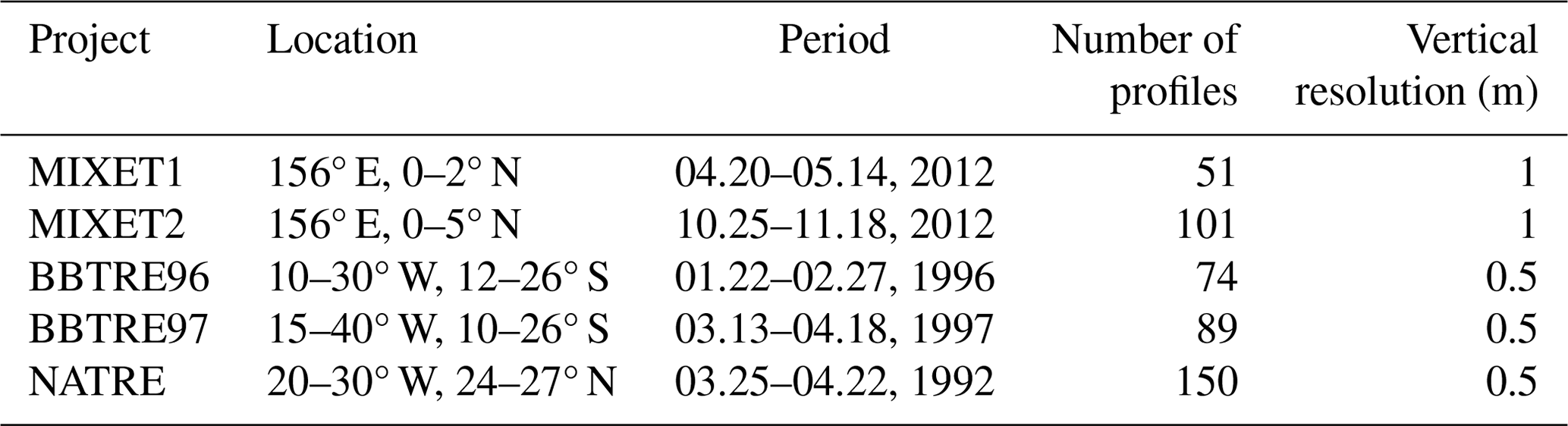
MIXET: MIXing in the Equatorial Thermocline (Waterhouse et al., 2014; Richards et al., 2015). BBTRE: Brazil Basin Tracer Release Experiment (Polzin et al., 1997). NATRE: North Atlantic Tracer Release Experiment (St. Laurent and Schmitt, 1999; Polzin and Ferrari, 2004).

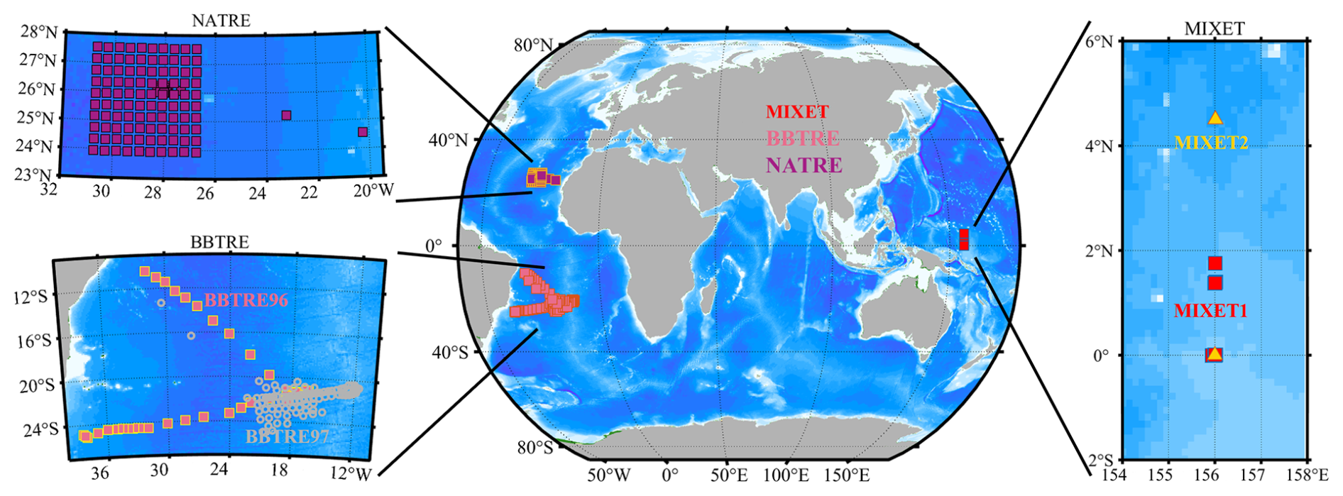
Figure 1 Station locations of the projects used in this study.

2.2 Identifying turbulent mixing and salt finger mixing

The profiles are divided into half-overlapped patches for further analysis. Following St. Laurent and Schmitt (1999), we choose 10 times the vertical resolution as the patch size – that is, 10 m (5 m) for projects with a vertical resolution of about 1 m (0.5 m). We first examine if and which type of double diffusion is favorable for each patch in a thermodynamical sense by the Turner angle, Tu = tan⁻¹($-\mathit{\alpha }{\mathit{\theta }}_z-\mathit{\beta }{S}_z,-\mathit{\alpha }{\mathit{\theta }}_z+\mathit{\beta }{S}_z$) (Ruddick, 1983). Here, α and β are the thermal expansion and saline contraction coefficients, respectively; θ_z and S_z are the vertical gradients of the original temperature and salinity profiles, respectively; and atan⁻¹ is the four-quadrant inverse tangent. Tu varies between −180 and 180°, categorizing the water column into four thermodynamical regimes: doubly stable (|Tu| < 45°), salt-finger-favorable (45° < Tu < 90°), diffusive-convection-favorable (−90° < Tu < −45°), and gravitationally unstable (|Tu| > 90°) (Ruddick, 1983). Tu is related to the density ratio R_ρ by $R_{\mathit{\rho }}=-\tan (\mathrm{Tu}+\mathrm{45}\mathit{°}$). We exclude weak double-diffusion signals (45° < Tu < 60° for salt-finger-favorable and −60° < Tu < −45° for diffusive-convection-favorable) for further identification.

In addition to the specific thermodynamical precondition, distinct statistical features are presented when double-diffusion-induced mixing is dominant. First, Re_b is found to be no greater than O(10) for active double diffusion (Inoue et al., 2007) and salt fingers are rare for Re_b between 10 and 10⁴ (St. Laurent and Schmitt, 1999). Re_b is defined as $R{e}_{\mathrm{b}}=\mathit{\epsilon }/\mathit{\nu }{N}^{\mathrm{2}}$, where ν is the molecular viscosity coefficient. Moreover, double diffusion generally corresponds to elevated χ_θ (St. Laurent and Schmitt, 1999; Inoue et al., 2007), and the magnitude of χ_θ is significantly larger than ε when double diffusion prevails and turbulence is absent (Nagai et al., 2015). Therefore, we use Re_b < 25 and $\left|{\mathit{\chi }}_{\mathit{\theta }}\right|/\left|\mathit{\epsilon }\right|\ge$ 7 as additional criteria for the identification of double diffusion.

For a doubly stable and gravitationally unstable water column, since their thermodynamical condition excludes the existence of double diffusion, we assume the mixing within the column is solely induced by turbulence. The most prominent difference between turbulence patches with |Tu| < 45° and those with |Tu| > 90° is that Re_b of the former is significantly smaller than that of the latter. And |Tu| > 90° generally means the presence of overturns. Therefore, the former patches are grouped as “weak turbulence” and the latter represent “energetic turbulence”.

Based on Tu, Re_b, and $\left|{\mathit{\chi }}_{\mathit{\theta }}\right|/\left|\mathit{\epsilon }\right|$, we classify the dominant mixing mechanisms into four types: weak turbulence (|Tu| < 45° with small Re_b), energetic turbulence (| Tu| > 90° with large Re_b), salt fingers (60° < Tu < 90°, Re_b < 25 and $\left|{\mathit{\chi }}_{\mathit{\theta }}\right|/\left|\mathit{\epsilon }\right|\ge$ 7), and diffusive convection (−90° < Tu < −60°, Re_b < 25 and $\left|{\mathit{\chi }}_{\mathit{\theta }}\right|/\left|\mathit{\epsilon }\right|\ge$ 7). Diffusive convection prevails mostly in the polar and subpolar regions (van der Boog et al., 2021); thus, it is rarely identified in this study (Sect. 3). As a result, diffusive convection is excluded from further analysis.

2.3 Estimating dissipation ratios and eddy diffusivities for turbulent mixing and salt finger mixing

The dissipation ratio Γ is defined as

$$\begin{array}{}\text{(1)}& \mathrm{\Gamma }={\displaystyle \frac{{\mathit{\chi }}_{\mathit{\theta }}{N}^{\mathrm{2}}}{\mathrm{2}\mathit{\epsilon }{\mathit{\theta }}_z^{\mathrm{2}}}}\end{array}$$

for turbulent mixing and salt finger mixing (Oakey, 1985). Based on the production–dissipation balances for TKE and thermal variance (Osborn and Cox, 1972; Osborn, 1980), and introducing R_ρ and the density flux ratio $r=\mathit{\alpha }{K}_{\mathit{\theta }}{\mathit{\theta }}_z/\mathit{\beta }{K}_{\mathrm{S}}{S}_z=K_{\mathit{\theta }}/K_S\cdot R_{\mathit{\rho }}$, we get

$$\begin{array}{}\text{(2)}& \begin{array}{rl}\mathrm{\Gamma }& ={\displaystyle \frac{{\mathit{\chi }}_{\mathrm{T}}{N}^{\mathrm{2}}}{\mathrm{2}\mathit{\epsilon }{\mathit{\theta }}_z^{\mathrm{2}}}}=\left({\displaystyle \frac{R_{\mathrm{f}}}{\mathrm{1}-R_{\mathrm{f}}}}\right){\displaystyle \frac{K_{\mathit{\theta }}}{K_{\mathit{\rho }}}}=\left({\displaystyle \frac{R_{\mathrm{f}}}{\mathrm{1}-R_{\mathrm{f}}}}\right)\\ & \left({\displaystyle \frac{R_{\mathit{\rho }}-\mathrm{1}}{R_{\mathit{\rho }}}}\right)\left({\displaystyle \frac{r}{r-\mathrm{1}}}\right),\end{array}\end{array}$$

which is applicable to both turbulent mixing and salt finger mixing (please refer to St. Laurent and Schmitt, 1999, for the specific derivation).

For turbulent mixing only, $K_{\mathrm{S}}=K_{\mathit{\theta }}=K_{\mathit{\rho }}$. Then, Eq. (2) leads to

$$\begin{array}{}\text{(3)}& {\mathrm{\Gamma }}^{\mathrm{T}}={\displaystyle \frac{{\mathit{\chi }}_{\mathrm{T}}{N}^{\mathrm{2}}}{\mathrm{2}\mathit{\epsilon }{\mathit{\theta }}_z^{\mathrm{2}}}}={\displaystyle \frac{R_{\mathrm{f}}}{\mathrm{1}-R_{\mathrm{f}}}}\end{array}$$

and

$$\begin{array}{}\text{(4)}& K_{\mathit{\theta }}^{\mathrm{T}}=K_{\mathrm{S}}^{\mathrm{T}}=K_{\mathit{\rho }}^{\mathrm{T}}={\mathrm{\Gamma }}^{\mathrm{T}}{\displaystyle \frac{\mathit{\epsilon }}{N^{\mathrm{2}}}},\end{array}$$

where the superscript “T” indicates turbulent mixing.

However, for salt finger mixing only, with $\frac{R_{\mathrm{f}}}{\mathrm{1}-R_{\mathrm{f}}}=-\mathrm{1}$ (St. Laurent and Schmitt, 1999), Eq. (2) yields

$$\begin{array}{}\text{(5)}& {\mathrm{\Gamma }}^{\mathrm{F}}={\displaystyle \frac{{\mathit{\chi }}_{\mathrm{T}}{N}^{\mathrm{2}}}{\mathrm{2}\mathit{\epsilon }{\mathit{\theta }}_z^{\mathrm{2}}}}=-{\displaystyle \frac{K_{\mathit{\theta }}}{K_{\mathit{\rho }}}}=-\left({\displaystyle \frac{R_{\mathit{\rho }}-\mathrm{1}}{R_{\mathit{\rho }}}}\right)\left({\displaystyle \frac{r^{\mathrm{F}}}{r^{\mathrm{F}}-\mathrm{1}}}\right),\end{array}$$

which cannot be used directly to estimate the salt-finger-induced eddy diffusivities. They are estimated separately by introducing R_ρ and $r^{\mathrm{F}}=R_{\mathit{\rho }}{\mathrm{\Gamma }}^{\mathrm{F}}/\left(R_{\mathit{\rho }}{\mathrm{\Gamma }}^{\mathrm{F}}+R_{\mathit{\rho }}-\mathrm{1}\right)$ (St. Laurent and Schmitt, 1999; Schmitt et al., 2005; Inoue et al., 2007):

$$\begin{array}{}\text{(6)}& \begin{array}{rl}& K_{\mathit{\theta }}^{\mathrm{F}}=\left({\displaystyle \frac{R_{\mathit{\rho }}-\mathrm{1}}{R_{\mathit{\rho }}}}\right)\left({\displaystyle \frac{r^{\mathrm{F}}}{\mathrm{1}-r^{\mathrm{F}}}}\right){\displaystyle \frac{\mathit{\epsilon }}{N^{\mathrm{2}}}}={\mathrm{\Gamma }}_{\mathit{\theta }}^{\mathrm{F}}{\displaystyle \frac{\mathit{\epsilon }}{N^{\mathrm{2}}}},\\ & K_{\mathrm{S}}^{\mathrm{F}}={\displaystyle \frac{R_{\mathit{\rho }}-\mathrm{1}}{\mathrm{1}-r^{\mathrm{F}}}}{\displaystyle \frac{\mathit{\epsilon }}{N^{\mathrm{2}}}}={\mathrm{\Gamma }}_{\mathrm{S}}^{\mathrm{F}}{\displaystyle \frac{\mathit{\epsilon }}{N^{\mathrm{2}}}}.\end{array}\end{array}$$

Note that all these equations are written in forms analogical to the Osborn relation for turbulent mixing. ${\mathrm{\Gamma }}_{\mathit{\theta }}^{\mathrm{F}}$ and ${\mathrm{\Gamma }}_{\mathrm{S}}^{\mathrm{F}}$ are two artificial “mixing efficiencies”, which are actually $\left(\frac{R_{\mathit{\rho }}-\mathrm{1}}{R_{\mathit{\rho }}}\right)\left(\frac{r^{\mathrm{F}}}{\mathrm{1}-r^{\mathrm{F}}}\right)$ and $\frac{R_{\mathit{\rho }}-\mathrm{1}}{\mathrm{1}-r^{\mathrm{F}}}$ before $\mathit{\epsilon }/N^{\mathrm{2}}$ for $K_{\mathit{\theta }}^{\mathrm{F}}$ and $K_{\mathrm{S}}^{\mathrm{F}}$ estimation. ${\mathrm{\Gamma }}_{\mathit{\theta }}^{\mathrm{F}}$ is the same as Γ^F, while ${\mathrm{\Gamma }}_{\mathrm{S}}^{\mathrm{F}}$ is further derived based on R_ρ and r^F: ${\mathrm{\Gamma }}_{\mathrm{S}}^{\mathrm{F}}={\mathrm{\Gamma }}^{\mathrm{F}}\cdot R_{\mathit{\rho }}/r^{\mathrm{F}}$. Investigating the statistic features of ${\mathrm{\Gamma }}_{\mathit{\theta }}^{\mathrm{F}}$ and ${\mathrm{\Gamma }}_{\mathrm{S}}^{\mathrm{F}}$ can be practically useful when estimating $K_{\mathit{\theta }}^{\mathrm{F}}$ and $K_{\mathrm{S}}^{\mathrm{F}}$ solely based on ε and N².

3 Statical features of turbulent mixing and salt finger mixing

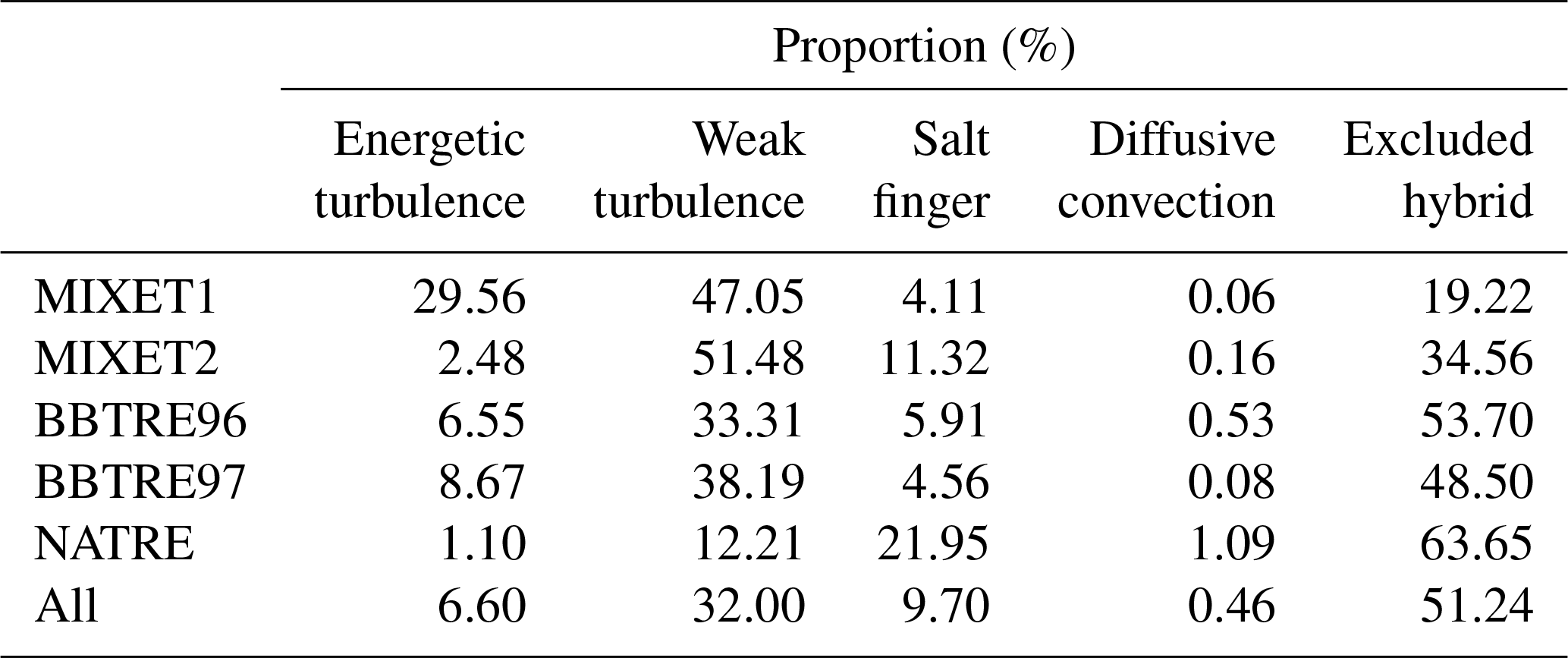
Figure 2 suggests that water properties vary greatly for the five projects, and Table 2 lists the proportions of patches for each mixing type. For the MIXET projects in the western equatorial Pacific, the Tu distribution in spring (MIXET1) shows a shape distinct from the autumn one (MIXET2). In spring, Tu shows double peaks at −30 and 110°, suggesting that mixing is alternately dominated by weak and energetic turbulence, although the contribution of the salt finger accounts for 4.1 % of the total patches and cannot be neglected. However, the autumn distribution is obviously unimodal, peaking at ∼ 45°, and the dominant mixing types are first weak turbulence and second salt finger mixing (∼ 51.5 % and 11.3 %, respectively), with negligible energetic turbulence and diffusive convection. For the BBTRE projects, although they are conducted in different years, the operating seasons are similar: one in late summer and the other early autumn (Southern Hemisphere), so the seasonal variation cannot be studied. Their Tu distributions are similarly bimodal, with a leading peak at 70° and a weak one at −40°, suggesting that the waters are mostly salt-finger-favorable (although only about 5.9 % is confirmed to be a salt finger) and stable (33.3 %), with rare energetic turbulence and neglectable diffusive-convection-favorable contribution. For NATRE, the salt finger overwhelms the others, occupying more than 21 % of the total patches; weak and energetic turbulence together hold 13.3 %, with the diffusive-convection-favorable type still being negligible (1 %). For BBTRE and NATRE, although a large proportion of the patches have 45° < Tu < 90° and are hence salt-finger-favorable, most of them have elevated Re_b; thus, we infer these mixing events to be hybrids of a salt finger and turbulence but dominated by turbulence. These patches are excluded from analysis to highlight the difference between turbulent and salt finger mixing. Only a few patches are chosen as effective salt finger events. Therefore, as concluded in the following section (Sect. 5.3), it is turbulent mixing that dominates the observed microstructures, in line with the results based on NATRE (St. Laurent and Schmitt, 1999). For these five projects, only 9.7 % of patches show clear salt finger features. Weak turbulence has a higher percentage (32.0 %), followed by 6.6 % of energetic turbulence. Diffusive convection occurs in less than 0.5 % of the total patches and is therefore negligible. Although dominated by turbulent mixing, the rest of the patches, more than 50 %, are hybrids of different mixing types and are excluded from the analysis.

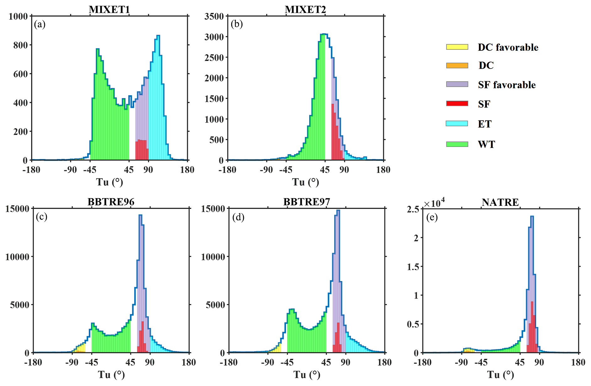
Figure 2 Histograms of patch-averaged Tu for different projects. Different Tu ranges of mixing types are marked by different colors: yellow for diffusive-convection-favorable (DC favorable; −90° < Tu < −60°), light purple for salt-finger-favorable (SF favorable; 60° < Tu < 90°), cyan for energetic turbulence (ET), and green for weak turbulence (WT). The red and orange bars denote the actual number of patches of salt fingers (SF) and diffusive convection (DC) selected by two more criteria, Re_b < 25 and $\left|{\mathit{\chi }}_{\mathit{\theta }}\right|/\left|\mathit{\epsilon }\right|\ge$ 5, respectively.

Table 2 Proportions of patches with energetic turbulence, weak turbulence, salt finger, diffusive convection, and hybrid mixing types (turbulence and salt finger, or turbulence and diffusive convection) compared to the total number of patches for each project and the sums for all the projects. Patches with hybrid mixing types are excluded from analysis.

We compare the statistical differences of Re_b, ε, N², and χ_θ for energetic turbulence, weak turbulence, and salt fingers by analyzing all the patches from the five projects (Fig. 3). The salt finger patches are featured with the weakest turbulence intensity compared with weak and energetic turbulence patches, whose median Re_b values are 5.0, 18.2, and 132.7, respectively. The median Re_b of energetic turbulence is slightly smaller than that reported in Mashayek et al. (2017) but close to the findings of Ijichi and Hibiya (2018). Since the samples given here are from five different projects, their Re_b distributions are actually different: for MIXET projects, the median Re_b of energetic turbulence is small, only about 50, while the rest of the projects generally have a median Re_b around 200 for energetic turbulence. The variations of ε for different mixing types differ little, mostly ranging from 3 × 10⁻¹² to 3 × 10⁻⁸ W kg⁻¹. Although the median ε for energetic turbulence is not obviously different from those for weak turbulence and salt fingers (7.8 × 10⁻¹¹, 7.9 × 10⁻¹¹ and 1.1 × 10⁻¹⁰ W kg⁻¹, respectively), it should be noted that most large ε values are induced by energetic turbulence. Distributions of χ_θ for weak turbulence and energetic turbulence differ little, but χ_θ of a salt finger is clearly greater in terms of variation ranges (salt finger: 3 × 10⁻¹¹–10⁻⁷ °C² s⁻¹; weak turbulence and energetic turbulence: 10⁻¹³–10⁻⁷ °C² s⁻¹) and median values (salt finger: 1.8 × 10⁻⁹ °C² s⁻¹; energetic turbulence and weak turbulence: 1.5 × 10⁻¹¹ °C² s⁻¹). Earlier studies considered the doubly stable regime to involve no mixing or excluded it from analysis (Inoue et al., 2007); however, besides some slight differences of proportion in large χ_θ and ε, energetic turbulence and weak turbulence share very similar distributions of χ_θ and ε (Fig. 3b, d), suggesting that the doubly stable regime does not mean an absence of turbulence and should be dominated by weak turbulence. Stratification also presents different features for different mixing types. Energetic turbulence has the weakest stratification with a median of 6.1 × 10⁻⁷ s⁻², only $\mathrm{1}/\mathrm{5}$ of that for weak turbulence. And the salt finger presents the strongest stratification (1.9 × 10⁻⁵ s⁻²). Clearly, the identified patches with energetic turbulence, weak turbulence, and salt fingers have distinct turbulent features, verifying the validity of the chosen criteria.

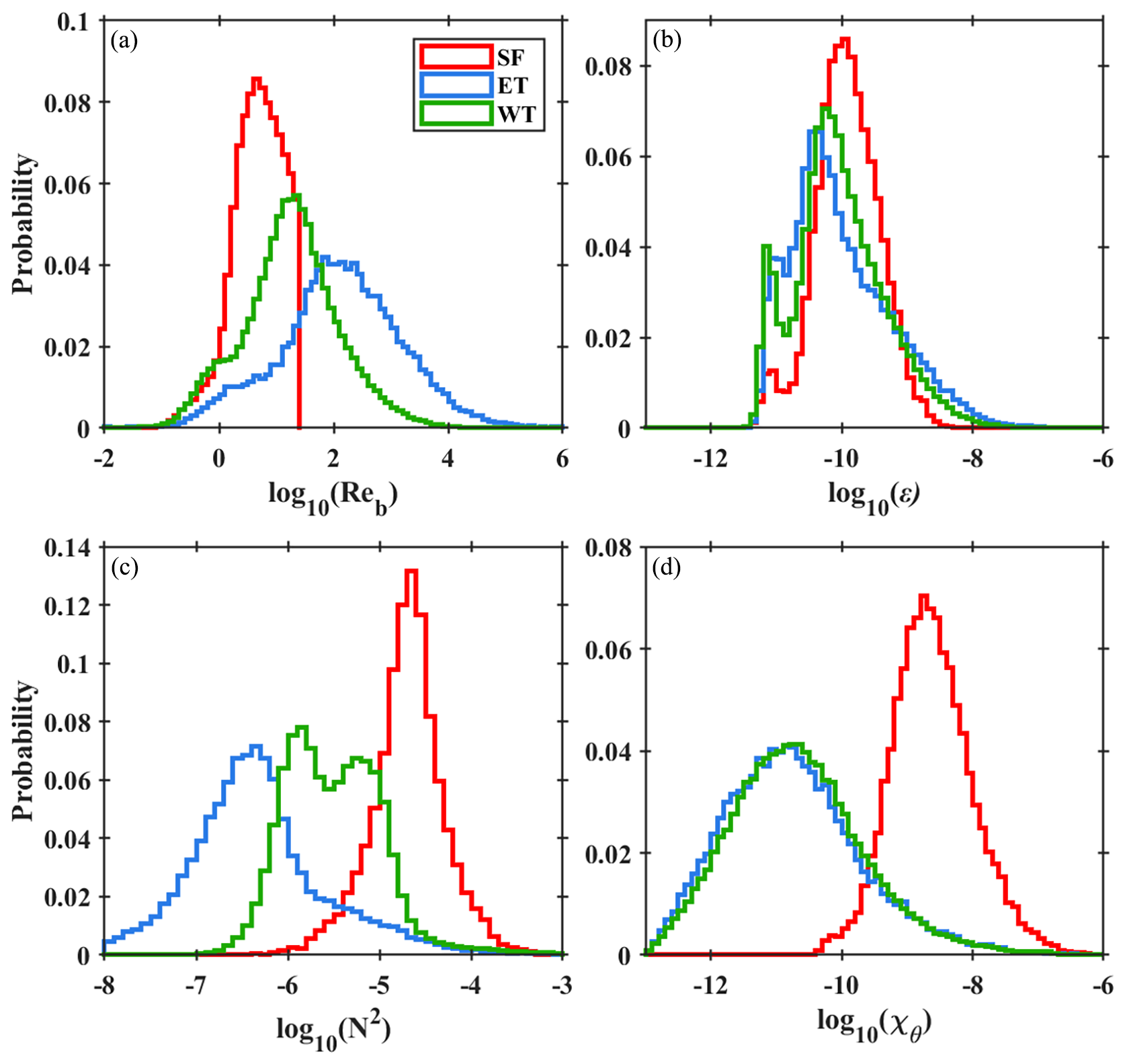
Figure 3 Probability-normalized histograms of log₁₀(Re_b) (a), log₁₀(ε) (b), log₁₀(N²) (c), and log₁₀(χ_θ) (d) for different mixing types: SF (salt finger), ET (energetic turbulence), and WT (weak turbulence). Data from the five projects are taken as the whole collection.

A normalized occurrence frequency is calculated to quantify the vertical variation of each mixing type (Fig. 4). Taking energetic turbulence as an example, we first divide the number of energetic turbulence patches in each depth bin by the total number of energetic turbulence patches in the whole project; then, to eliminate the vertical variation of observation frequency, we divide the results by the total number of patches within the same depth bin. This occurrence frequency is eventually normalized between 0 and 1 using its maximum. Consistent with observations in the upper thermocline (Schmitt et al., 2005; van der Boog et al., 2021), salt fingers mostly prevail in the upper 500–1000 m for all projects, with their occurrence frequencies reaching 1. For the MIXET projects and NATRE, the occurrence frequencies of a salt finger gradually become weak and near zero with depth increasing to the seafloor. However, for the BBTRE projects, salt fingers sharply disappear between 1000 and 2000 m and re-occur at greater depth (see Fig. 10). The depth-colored T–S diagrams suggest that the vertical transition of different water masses is responsible for the sudden disappearance of the salt finger (Fig. 5). It is clear to see that both θ and S decrease with depth in most water columns, providing the basic precondition for a salt finger. However, this tendency changes obviously between 1000 and 2000 m. At this depth range, θ changes little, but S increases drastically by at least 0.5; this prevents the occurrence of a salt finger. This depth is just where the fresher Antarctic Intermediate Water transits to the North Atlantic Deep Water. Consequently, the occurrence frequency of a salt finger is severely weakened at this depth. In contrast to salt fingers, energetic turbulence generally becomes more prevalent with increasing depth for most projects. The remarkably weak background stratification may contribute a lot to the prevalence of energetic turbulence at depth, where even a weak perturbation can fully develop.

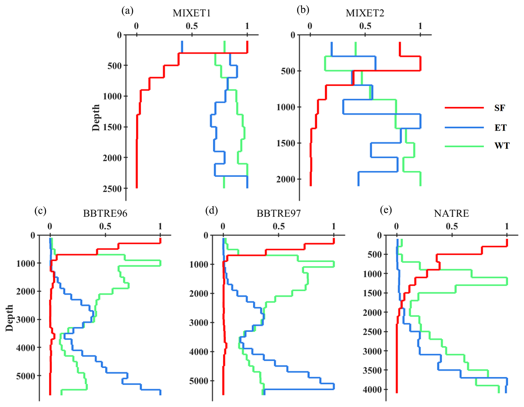
Figure 4 Vertical variations of the normalized occurrence frequency of a salt finger (SF), energetic turbulence (ET), and weak turbulence (WT) for the five projects. The depth range is from 100 m to the deepest measurements, with a bin size of 200 m.

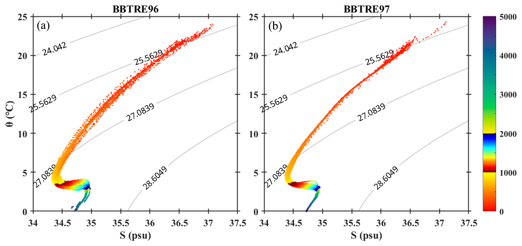
Figure 5 T–S diagrams for BBTRE96 and BBTRE97. Color indicates patch depth, and the contour indicates isopycnic.

4 Γ variation of turbulence and salt fingers

4.1 Γ variation of turbulence

4.1.1 Vertical variation

We explore the variation of Γ^T first. Figure 6 suggests that Γ^T varies in a distinct way for different projects. Results for the MIXET projects suggest that Γ^T in the western equatorial Pacific is significantly seasonally variable. In spring (MIXET1), Γ^T of energetic turbulence varies between 2.5 × 10⁻² and 1.7 (10th–90th percentiles) with a median of 0.23, smaller than that of weak turbulence ranging between 1.4 × 10⁻¹ and 2.8 and peaking at 0.52. Γ^T in autumn is significantly elevated (MIXET2), and the medians and variation ranges for energetic turbulence and weak turbulence are 0.41 and from 3.4 × 10⁻² to 8.8 as well as 0.58 and from 1.7 × 10⁻¹ to 2.3, respectively. For the BBTRE projects, Γ^T of weak turbulence varies little between different years, with most patches varying between 10⁻² and 10, although the median value in 1997 (0.35) was greater than that in 1996 (0.20). Γ^T of energetic turbulence is larger in 1997 than that in 1996, with median values of 0.48 and 0.20, respectively. Estimates from NATRE also suggest that Γ^T largely scatters between 10⁻² and 10 for most patches; the median Γ^T values are 0.33 and 0.50 for energetic turbulence and weak turbulence, respectively. To summarize, besides the BBTRE and energetic turbulence of the MIXET projects showing a median value close to 0.2, the rest of the estimates are all clearly greater than 0.2. Γ^T for the five projects mostly varies within 3 orders of magnitude from 10⁻² to 10, in line with other observations (Ijichi and Hibiya, 2018; Vladoiu et al., 2021; Li et al., 2023).

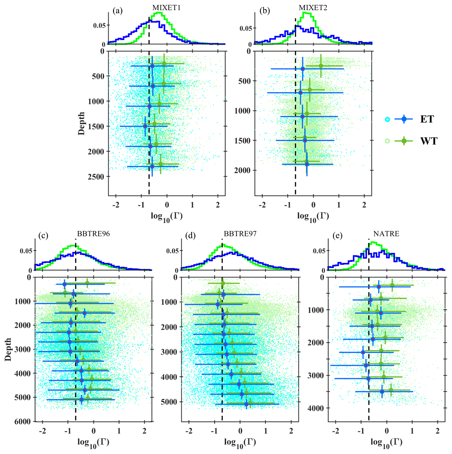
Figure 6 Variations of Γ^T of energetic turbulence (ET) and weak turbulence (WT). Each panel consists of two sub-panels, with the upper one showing a probability-normalized histogram of Γ^T and the lower one being Γ^T–depth scatter; the median value of each depth bin is marked by a larger, darker dot overlying a cross marker, with a horizontal bar indicating the 10th to 90th percentile range and vertical bar indicating the depth bin range. The median Re_b values are compared between energetic turbulence and weak turbulence at each depth bin, and the median Γ^T corresponding to the larger Re_b is marked by a red dot. The conventional value of Γ^T, namely 0.2, is represented by the dashed black line.

For different projects, Γ^T varies with depth in different ways. For MIXET1, Γ^T of both energetic turbulence and weak turbulence fluctuates around the statistical median values weakly. For MIXET2, the depth median Γ^T of energetic turbulence varies between 0.2 and 0.7, with a slight increase with depth. However, Γ^T of weak turbulence shows a clear decrease from 2.5 at 300 m to 0.6 at 1400 m; then, it slightly increases to 0.8 at 1900 m. The Γ^T of weak turbulence for BBTRE96 fluctuates around 0.2 in the upper 300 m, and then it increases to ∼ 1 at 4400 m and decreases to ∼ 0.6 at 5200 m. The scenario for energetic turbulence shows a similar picture. Γ^T of weak turbulence for BBTRE97 departs little from 0.2 at depths above 1800 m, then monotonically increases to ∼ 2.3 at the deepest depth around 5200 m. Γ^T of energetic turbulence varies in a similar way in the vertical direction, except the depth where the trend change is 3000 m. For NATRE, Γ^T of energetic turbulence first decreases from 0.6 to 0.1 at 2300 m, then increases to 0.8 at 3500 m. As for weak turbulence, Γ^T stays around 0.8 between 600 and 3000 m and then increases beyond unity at 3500 m. In terms of the general trend by linearly fitting Γ^T with depth, the five projects show two distinct vertical patterns of Γ^T: one is the downward-decreasing pattern represented by the MIXET projects, and the other is the downward-increasing one suggested by the rest of the projects over the midlatitudes of the Atlantic. Downward-increasing Γ^T was also reported by Ijichi and Hibiya (2018). Their data collection sites were spread over middle to high latitudes of the Pacific and Southern Ocean. Γ^T also presented a clear downward increase in the upper 500 m of the South China Sea north of 10° N (Li et al., 2023). Combining all these observational results, we suggest that Γ^T in the equatorial area should be treated differently, since it may decrease with depth, contrary to the downward increase away from the Equator.

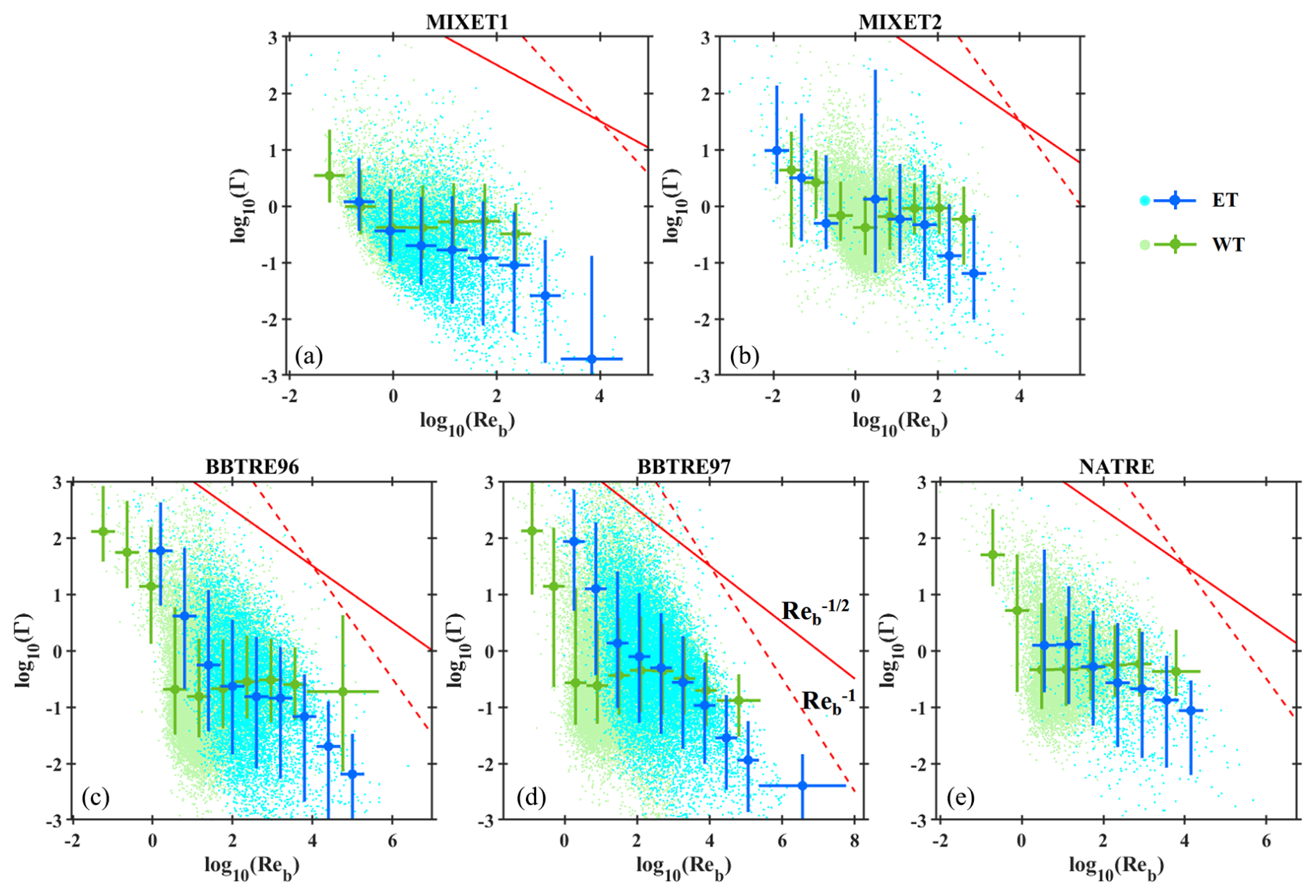
Figure 7 Relations between Γ^T and Re_b for energetic turbulence (ET) and weak turbulence (WT). Overlying the light-colored scatter of individual patches, Re_b-binned median values are marked by large darker dots, and the bin size and the 10th–90th percentile range of Γ^T are denoted by the horizontal and vertical bars, respectively. The solid and dashed red lines mark ${\mathrm{\Gamma }}^{\mathrm{T}}\propto R{e}_{\mathrm{b}}^{-\mathrm{1}/\mathrm{2}}$ and ${\mathrm{\Gamma }}^{\mathrm{T}}\propto R{e}_{\mathrm{b}}^{-\mathrm{1}}$, respectively.

The full-depth statistics of the five projects disagree regarding whether Γ^T is larger for energetic turbulence or weak turbulence. However, when comparing Γ^T values of energetic turbulence and weak turbulence in the same depth bin, Γ^T of energetic turbulence is mostly smaller than that of weak turbulence. Considering that Re_b is reported to modulate the variation of Γ^T (Mashayek et al., 2017; Monismith et al., 2018) and that energetic turbulence and weak turbulence have clearly different Re_b distributions (Fig. 3), we found that energetic turbulence with smaller Γ^T generally has larger Re_b than weak turbulence, indicating a negative correlation between Γ^T and Re_b.

4.1.2 Relation between Γ^T, Re_b, and R_OT

We then investigate the relations between Γ^T and Re_b for energetic turbulence and weak turbulence (Fig. 7). For MIXET1, Γ^T of weak turbulence first decreases from 3.5 to 0.5 with Re_b increasing from 0.1 to 1, suggesting a relation of ${\mathrm{\Gamma }}^{\mathrm{T}}\propto R{e}_{\mathrm{b}}^{-\mathrm{1}}$, and then it weakly increases to 0.7 with Re_b reaching 100; a weak decrease in line with ${\mathrm{\Gamma }}^{\mathrm{T}}\propto R{e}_{\mathrm{b}}^{-\mathrm{1}/\mathrm{2}}$ can be observed for Re_b > 100. For energetic turbulence, Γ^T generally decreases with Re_b, indicating ${\mathrm{\Gamma }}^{\mathrm{T}}\propto R{e}_{\mathrm{b}}^{-\mathrm{1}/\mathrm{2}}$; this relation is consistent with the observations in the western Mediterranean Sea (Vladoiu et al., 2021). The pattern for MIXET2 is similar to that for MIXET1, although Γ^T of weak turbulence decreases at a smaller rate when Re_b is small and indicates ${\mathrm{\Gamma }}^{\mathrm{T}}\propto R{e}_{\mathrm{b}}^{-\mathrm{1}/\mathrm{2}}$. Excluding the bins with few data points, Γ^T of weak turbulence for BBTRE96 shows a weak increase from 0.2 to 0.3 as Re_b grows from 10 to 10³ and a weak decrease with Re_b exceeding 10³. Γ^T and Re_b of weak turbulence for BBTRE97 show similar relationships as those for BBTRE96. The weak turbulence variations for BBTRE are the same as the estimates reported by Ijichi et al. (2020), and the shape is similar to the upper bound of the nonmonotonic Γ^T∼ Re_b relation proposed by Mashayek et al. (2017). It is notable that the scenario for energetic turbulence is distinct; Γ^T generally decreases from 5 to less than 0.1 with Re_b between 10 and 2.5 × 10⁴ for BBTRE96, forming a fitting slope steeper than $-\mathrm{1}/\mathrm{2}$ but flatter than −1. Γ^T of energetic turbulence for BBTRE97 also shows a similar decrease with Re_b. Except for the bins with few samples when Re_b < 1 and Re_b > 10⁴, Γ^T of weak turbulence for NATRE generally increases from 0.5 to 0.7, while Γ^T of energetic turbulence monotonically decreases from ∼ 1 at Re_b= 10² to ∼ 0.1 at Re_b=10⁴, suggesting ${\mathrm{\Gamma }}^{\mathrm{T}}\propto R{e}_{\mathrm{b}}^{-\mathrm{1}/\mathrm{2}}$.

Although Γ^T generally decreases with Re_b in most cases for the five projects, the decreasing rate varies with projects and Re_b ranges. There are several cases showing that Γ^T stays constant or even increases with Re_b. This suggests that Γ^T is not solely modulated by Re_b, and there may be other factors that influence Γ^T in a comparable or even dominating role relative to Re_b. R_OT is reported as a parameter that regulates Γ^T more strongly than Re_b, ${\mathrm{\Gamma }}^{\mathrm{T}}\propto R_{\mathrm{OT}}^{-\mathrm{4}/\mathrm{3}}$ (Ijichi and Hibiya, 2018). R_OT is the ratio of the Ozmidov scale L_O to the Thorpe scale L_T, $R_{\mathrm{OT}}=L_{\mathrm{O}}/L_{\mathrm{T}}$ with $L_{\mathrm{O}}={\mathit{\epsilon }}^{\mathrm{1}/\mathrm{2}}/N^{\mathrm{3}/\mathrm{2}}$ and $L_{\mathrm{T}}=\langle {\mathit{\delta }}_{\mathrm{T}}^{\mathrm{2}}{\rangle }^{\frac{\mathrm{1}}{\mathrm{2}}}$, where the Thorpe displacement δ_T is the depth difference of a water parcel between the original and sorted potential temperature profiles of an overturn. Overturns are identified by the cumulative Thorpe displacement ∑δ_T (Mater et al., 2015; Ijichi and Hibiya, 2018). Because the vertical resolution of temperature profiles is 1 or 0.5 m, overturns with a vertical size of O(1) m or smaller cannot be identified. Additionally, the identified overturns with a size smaller than 10 m or greater than 400 m are excluded from analysis because the former contain too few data points and the latter are possibly the vertical structures of different water masses instead of genuine turbulent overturns. We also estimate the overturn-averaged Tu, Γ^T, and Re_b. Due to the coarse vertical resolution of temperature profiles used in our study, only a few overturns meet the identification criteria for each project; as a result, the overturns of the five projects are taken as one collection (the total number of overturns is 3862).

Figure 8 shows the overturn-based relation between Γ^T and R_OT. Since most overturns are identified at depth, with only one-fifth shallower than 1000 m but more than one-third below 2000 m, the overturn-based Γ^T is clearly greater than 0.2, with a median value of 0.91. In Fig. 8, although overturns are evenly scattered in the R_OT–Γ^T space, the probability density shows that they are concentrated around two sites mostly, one with R_OT and Γ^T of 0.03 and 1.19 and the other with 0.56 and 0.53. These two clusters are distinctly characterized by Re_b, with the first location corresponding to Re_b < 160 (median value of 25) and the other to Re_b > 160 (median value of 835). For both clusters, the contours of probability density tilt at slopes of $-\mathrm{4}/\mathrm{3}$, confirming ${\mathrm{\Gamma }}^{\mathrm{T}}\propto R_{\mathrm{OT}}^{-\mathrm{4}/\mathrm{3}}$ is valid for each cluster. However, the general trend between R_OT and Γ^T for the whole data collection is much flatter, with a slope of only about $-\mathrm{1}/\mathrm{2}$. Comparing Re_b of the two clusters, it is easy to find that Re_b grows exponentially with R_OT. Therefore, the general variation of Γ^T with the growth of R_OT is not only influenced by R_OT, but also partly affected by Re_b. Supposing Γ^T is mostly modulated by these two parameters, and considering that the decrease in Γ^T with R_OT is significantly weakened by Re_b, this suggests a positive relation between Γ^T and Re_b.

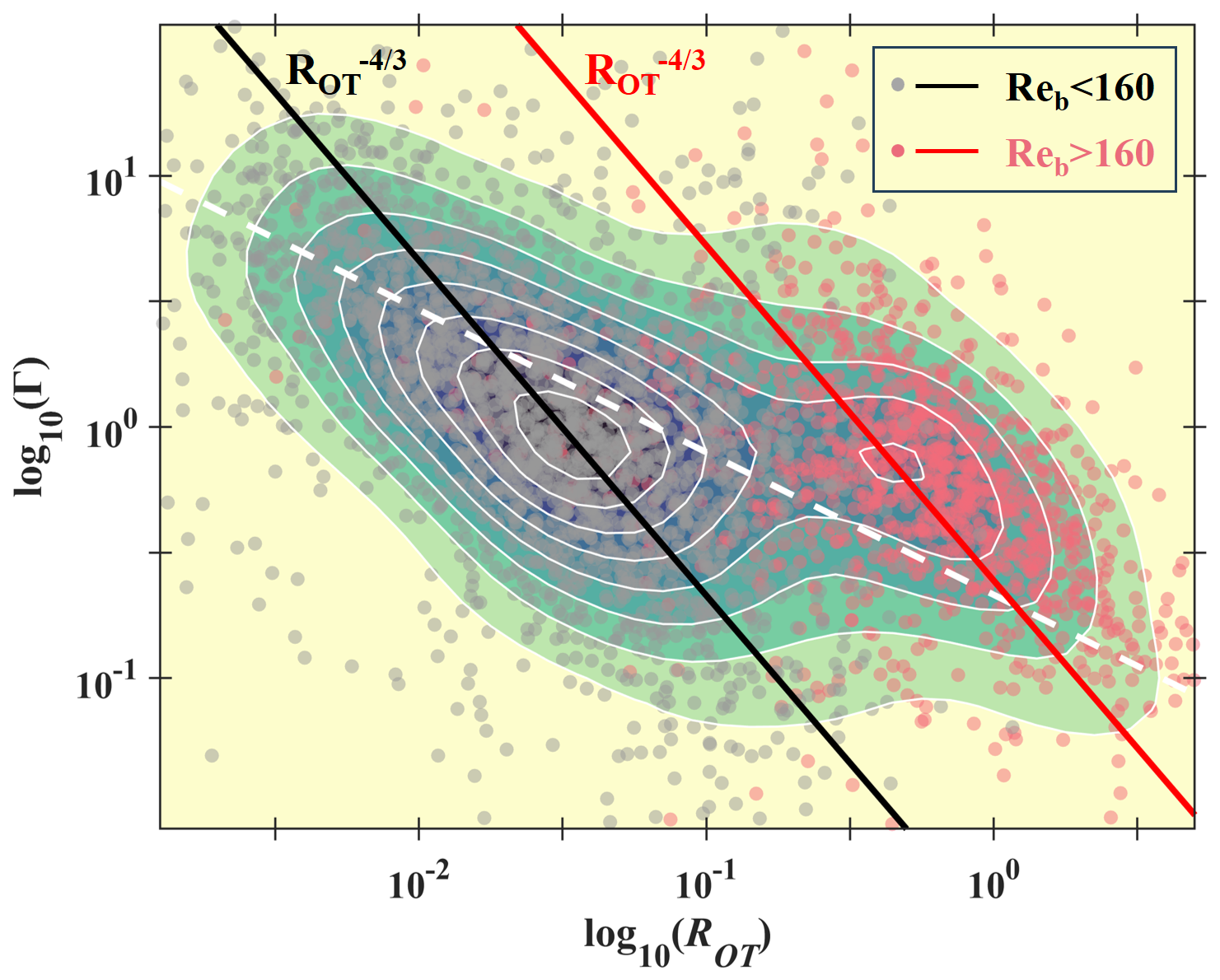
Figure 8 Relation between overturn-based Γ^T and R_OT; overturns from the five projects are considered. The shading describes the distribution of probability density, with yellow indicating minimum probability density and blue representing the maximum one. The overturns are correspondingly divided into two clusters: the gray dots have Re_b < 160 and the pink ones Re_b >  160. The black and red lines represent ${\mathrm{\Gamma }}^{\mathrm{T}}\propto R_{\mathrm{OT}}^{-\mathrm{4}/\mathrm{3}}$, crossing the centers of the two clusters. The dashed white line is the general relation between Γ^T and R_OT of the whole data collection.

Figure 9 shows the variation of the median value of Γ^T jointly binned by Re_b and R_OT. Note that most parts of the Re_b–R_OT space are null, with all the data gathered around a band originating from large Re_b and R_OT to small Re_b and R_OT. This confirms that Re_b and R_OT are positively correlated in general. As for the median Γ^T, although its value is scattered, its general pattern indicates that Γ^T grows fastest along a direction from small Re_b and large R_OT to large Re_b and small R_OT, suggesting that Γ^T is indeed positively correlated with Re_b and negatively correlated with R_OT. Assuming ${\mathrm{\Gamma }}^{\mathrm{T}}\propto R_{\mathrm{OT}}^{-\mathrm{4}/\mathrm{3}}\cdot R{e}_{\mathrm{b}}^c$, we substitute the median values of Γ^T, Re_b, and R_OT in Fig. 9 into this relation to fit the exponent c. The fitting results suggest c≈ 1/2 and a relation of Γ^T≈10${}^{-\mathrm{3}}\cdot R_{\mathrm{OT}}^{-\mathrm{4}/\mathrm{3}}\cdot R{e}_{\mathrm{b}}^{\mathrm{1}/\mathrm{2}}$. The isolines of this relation are shown in Fig. 9, which can capture the main variation of Γ^T well with Re_b and R_OT. Based on the microstructure measurements collected from the upper layer in the South China Sea, Li et al. (2023) presented a relation of ${\mathrm{\Gamma }}^{\mathrm{T}}\approx a{R}_{\mathrm{OT}}^{-\mathrm{4}/\mathrm{3}}\cdot R{e}_{\mathrm{b}}^{\mathrm{1}/\mathrm{2}}$, but a is around 0.02 in that region, which is 1 order of magnitude larger than the value presented here. This is because Re_b has a much smaller magnitude in the upper South China Sea, with most Re_b values varying between 10⁻¹ and 10³. Therefore, compared with the results in Li et al. (2023), the larger Re_b in this study leads to a relatively smaller a. On the other hand, the significant variation of a may suggest that some other parameters can influence Γ^T besides Re_b and R_OT.

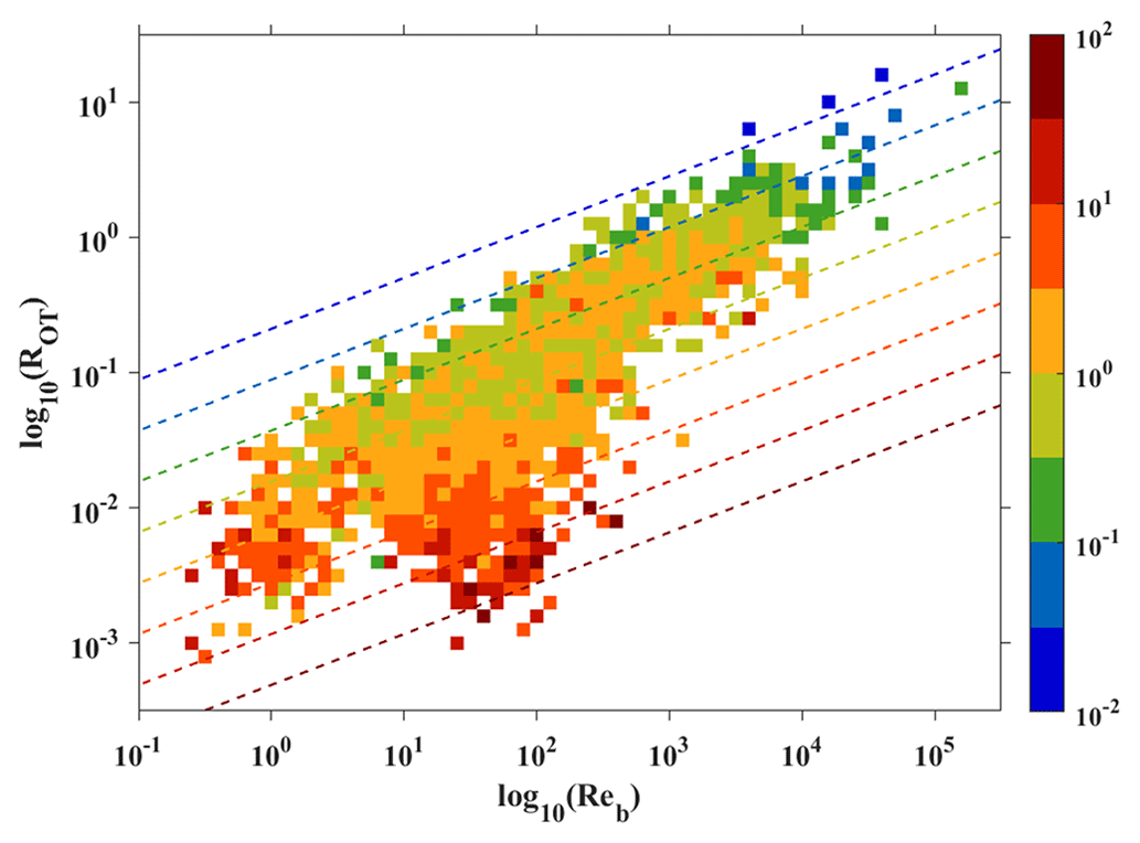
Figure 9 Variation of median Γ^T binned by R_OT and Re_b based on overturn estimates for the five projects. The color bar refers to the median Γ^T, and the dashed colored lines indicate the isolines of 10${}^{-\mathrm{3}}\cdot R_{\mathrm{OT}}^{-\mathrm{4}/\mathrm{3}}\cdot R{e}_{\mathrm{b}}^{\mathrm{1}/\mathrm{2}}$.

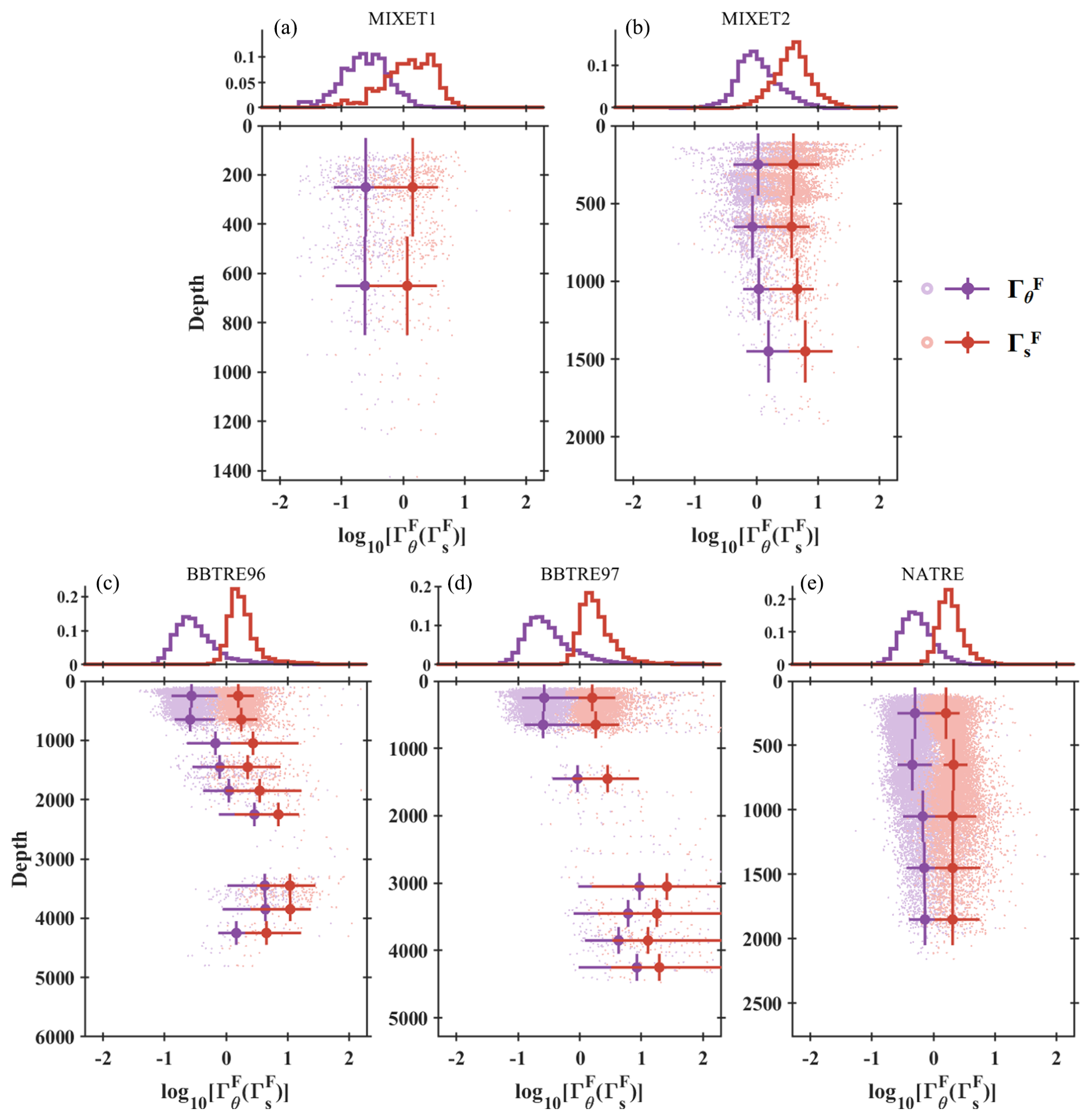
Figure 10 Variations of ${\mathrm{\Gamma }}_{\mathit{\theta }}^{\mathrm{F}}({\mathrm{\Gamma }}_{\mathrm{S}}^{\mathrm{F}}$) of a salt finger for the five projects. Each panel consists of two sub-panels, with the upper one showing the probability-normalized histograms of ${\mathrm{\Gamma }}_{\mathit{\theta }}^{\mathrm{F}}$ and ${\mathrm{\Gamma }}_{\mathrm{S}}^{\mathrm{F}}$ and the lower one being their vertical variations. The median value of each depth bin is marked by a larger, darker dot overlying a cross marker, with a horizontal bar indicating the 10th to 90th percentile range and a vertical bar indicating the depth bin range.

4.2 Γ variation of a salt finger

Γ^F has been widely used to distinguish salt fingers from turbulence, since its value is reported to be larger than the conventional Γ^T value of 0.2 (St. Laurent and Schmitt, 1999). However, the full-depth observations presented in this study and previous ones indicate that 0.2 is an underestimate of Γ^T, and the difference in the dissipation ratio between turbulent mixing and salt finger mixing in the deep water needs to be examined. Figure 10 presents the variations of ${\mathrm{\Gamma }}_{\mathit{\theta }}^{\mathrm{F}}$ and ${\mathrm{\Gamma }}_{\mathrm{S}}^{\mathrm{F}}$ with depth. Compared with Γ^T varying over 3 orders of magnitude, both ${\mathrm{\Gamma }}_{\mathit{\theta }}^{\mathrm{F}}$ and ${\mathrm{\Gamma }}_{\mathrm{S}}^{\mathrm{F}}$ are less variable and change by 2 orders of magnitude or as little as 1 order. The median ${\mathrm{\Gamma }}_{\mathit{\theta }}^{\mathrm{F}}$ for all samples from the five projects is 0.47, slightly smaller than the Γ^F observed in the diurnal thermocline of the Arabian Sea (0.65; Ashin et al., 2023), in the Kuroshio Extension Front (∼ 1; Nagai et al., 2015), and in the thermocline of the western tropical Atlantic (∼ 1.2; Schmitt et al., 2005). The median ${\mathrm{\Gamma }}_{\mathit{\theta }}^{\mathrm{F}}$ values for the five projects are distinct: 0.25, 0.29, and 0.28 for MIXET1, BBTRE96, and BBTRE97, similar to the conventional Γ^T value of 0.2 as well as 0.52 for NATRE, distinguishable from 0.2 but close to the observed Γ^T (Fig. 6), and 0.98 for MIXET2, significantly larger than 0.2 and different from the observed Γ^T (Fig. 6). This suggests that the dissipation ratio difference between turbulence and salt fingers is complex.

Vertically, ${\mathrm{\Gamma }}_{\mathit{\theta }}^{\mathrm{F}}$ for MIXET1 stays nearly constant at 0.25, while ${\mathrm{\Gamma }}_{\mathit{\theta }}^{\mathrm{F}}$ for MIXET2 first decreases from 1 to 0.7 in the upper 700 m and then slightly increases to 2 at 1500 m. ${\mathrm{\Gamma }}_{\mathit{\theta }}^{\mathrm{F}}$ presents a similar vertical trend for both BBTRE96 and BBTRE97: ${\mathrm{\Gamma }}_{\mathit{\theta }}^{\mathrm{F}}$ is small and stays constant within the upper 800 m, with a median of 0.28; with depth increasing to 3000 m, it significantly increases over orders of magnitude, with the median value reaching ∼ 10. It is weakened at deeper depth. Note that the relatively small median ${\mathrm{\Gamma }}_{\mathit{\theta }}^{\mathrm{F}}$ for the BBTRE projects is mainly caused by the dominant patches with small ${\mathrm{\Gamma }}_{\mathit{\theta }}^{\mathrm{F}}$ values in the upper 800 m, and ${\mathrm{\Gamma }}_{\mathit{\theta }}^{\mathrm{F}}$ at depth is actually very large and significantly greater than 0.2 or the observed Γ^T. The scenario for NATRE is similar to that for MIXET2, whose depth median ${\mathrm{\Gamma }}_{\mathit{\theta }}^{\mathrm{F}}$ remains nearly consistent around ∼ 0.5, although a very weak positive trend exists.

The “effective” salt dissipation ratio ${\mathrm{\Gamma }}_{\mathrm{S}}^{\mathrm{F}}$ tends to be obviously larger than ${\mathrm{\Gamma }}_{\mathit{\theta }}^{\mathrm{F}}$ (Fig. 10). With the overall median ${\mathrm{\Gamma }}_{\mathrm{S}}^{\mathrm{F}}$ of 1.87, the median values of ${\mathrm{\Gamma }}_{\mathrm{S}}^{\mathrm{F}}$ for the five projects are 1.35 (MIXET1), 3.98 (MIXET2), 1.67 (BBTRE96), 1.71 (BBTRE97), and 1.83 (NATRE), floating around the value reported in the thermocline of the western tropical Atlantic of ∼ 2.8 (Schmitt et al., 2005). ${\mathrm{\Gamma }}_{\mathrm{S}}^{\mathrm{F}}$ is strongly positively proportional to ${\mathrm{\Gamma }}_{\mathit{\theta }}^{\mathrm{F}}$, with the median values of ${\mathrm{\Gamma }}_{\mathrm{S}}^{\mathrm{F}}/{\mathrm{\Gamma }}_{\mathit{\theta }}^{\mathrm{F}}$ for the five projects being 5.1, 3.7, 6.3, 6.9, and 3.8, respectively. Thus, a general relation of ${\mathrm{\Gamma }}_{\mathrm{S}}^{\mathrm{F}}\approx$ 5${\mathrm{\Gamma }}_{\mathit{\theta }}^{\mathrm{F}}$ can be inferred. Due to this correlation, ${\mathrm{\Gamma }}_{\mathrm{S}}^{\mathrm{F}}$ presents vary similar vertical variation as ${\mathrm{\Gamma }}_{\mathit{\theta }}^{\mathrm{F}}$.

Note that ${\mathrm{\Gamma }}_{\mathrm{S}}^{\mathrm{F}}/{\mathrm{\Gamma }}_{\mathit{\theta }}^{\mathrm{F}}$ is equivalent to $R_{\mathit{\rho }}/r^{\mathrm{F}}$ (Eq. 6). Since R_ρ is relatively easy to calculate, it is an alternate way to infer the hard-to-measure r^F. R_ρ and r^F are the key parameters to estimate the dissipation ratios of heat and salt for a salt finger (Sect. 2.3). Therefore, many studies have tried to explore the relation of R_ρ and r^F based on theoretical derivations, laboratory experiments, and numerical simulations (Kelley, 1986; Kunze, 1987; Radko and Smith, 2012). Here, the R_ρ–r^F diagram colored by probability density for the five projects indicates that the salt finger patches are rather scattered (Fig. 11). However, the median r^F binned by R_ρ shows a clear nonmonotonic variability. For R_ρ increasing from 1 to 2.4, r^F decreases from ∼ 0.8 to 0.4; then, it gradually increases to 0.55 with R_ρ approaching 3.7. This correlation between R_ρ and r^F can be well fitted by

$$\begin{array}{}\text{(7)}& r^{\mathrm{F}}={\displaystyle \frac{\mathrm{0.79}\cdot R_{\mathit{\rho }}^{\mathrm{2}}-\mathrm{2.96}\cdot R_{\mathit{\rho }}+\mathrm{3.18}}{R_{\mathit{\rho }}^{\mathrm{2}}-\mathrm{3.26}\cdot R_{\mathit{\rho }}+\mathrm{3.46}}}.\end{array}$$

Compared with other correlation curves (Kelley, 1986; Kunze, 1987; Radko and Smith, 2012), all of them present an r^F decrease for R_ρ smaller than 2, although the variation range and rate differ. The most obvious discrepancy between them is that r^F tends to regain a larger value with R_ρ exceeding 2.4 in our study, while all the other curves decrease little to asymptote to a constant value. The observational result presented here falls in the area outlined by the existing results. For our results, the salt finger patches with R_ρ < 2.5 are abundant and mostly concentrated to indicate a negative correlation between R_ρ and r^F. It needs to be mentioned that patches with R_ρ > 2.5 are much more rare and sparsely distributed, making the increase in r^F in the larger R_ρ range need to be treated carefully.

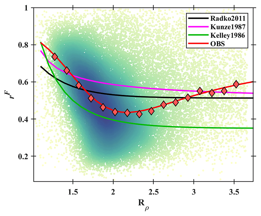
Figure 11 Relation between R_ρ and r^F. Salt finger patches from all five projects are considered. Dots are colored by probability density, with darker color indicating larger probability density. The median r^F values binned by R_ρ are marked by red diamonds with a black edge, and the red curve is the fitting curve. The black, orange, and purple curves are adopted from Radko and Smith (2012), Kunze (1987), and Kelley (1986), respectively.

We also investigate the relation between observed ${\mathrm{\Gamma }}_{\mathit{\theta }}^{\mathrm{F}}$ and Re_b (Fig. 12), which differs considerably between different projects. For MIXET1, a nearly linear decrease in ${\mathrm{\Gamma }}_{\mathit{\theta }}^{\mathrm{F}}$ (in logarithmic scale) from ∼ 1 to ∼ 0.1 can be easily observed for all patches with Re_b between 0.3 and 25, indicating ${\mathrm{\Gamma }}_{\mathit{\theta }}^{\mathrm{F}}\propto R{e}_{\mathrm{b}}^{-\mathrm{1}/\mathrm{2}}$. ${\mathrm{\Gamma }}_{\mathit{\theta }}^{\mathrm{F}}$ for MIXET2 with Re_b < 2.5 is also well fitted as ${\mathrm{\Gamma }}_{\mathit{\theta }}^{\mathrm{F}}\propto R{e}_{\mathrm{b}}^{-\mathrm{1}/\mathrm{2}}$, but ${\mathrm{\Gamma }}_{\mathit{\theta }}^{\mathrm{F}}$ for Re_b > 2.5 tends to remain constant at 0.7. For the BBTRE projects, when Re_b < 3, ${\mathrm{\Gamma }}_{\mathit{\theta }}^{\mathrm{F}}$ decreases at a larger rate than the MIXET projects, ${\mathrm{\Gamma }}_{\mathit{\theta }}^{\mathrm{F}}\propto R{e}_{\mathrm{b}}^{-\mathrm{1}}$, and ${\mathrm{\Gamma }}_{\mathit{\theta }}^{\mathrm{F}}$ stays almost unchanged when Re_b exceeds 3. ${\mathrm{\Gamma }}_{\mathit{\theta }}^{\mathrm{F}}$ for NATRE stays constant at 0.7 with most Re_b values ranging from 1 to 25. Due to the strong correlation between ${\mathrm{\Gamma }}_{\mathrm{S}}^{\mathrm{F}}$ and ${\mathrm{\Gamma }}_{\mathit{\theta }}^{\mathrm{F}}$, the dependence of ${\mathrm{\Gamma }}_{\mathrm{S}}^{\mathrm{F}}$ on Re_b is similar to that of ${\mathrm{\Gamma }}_{\mathit{\theta }}^{\mathrm{F}}$, although variation rates are different for some projects. Taking all the projects together, ${\mathrm{\Gamma }}_{\mathit{\theta }}^{\mathrm{F}}$ and ${\mathrm{\Gamma }}_{\mathrm{S}}^{\mathrm{F}}$ decrease with Re_b in general; however, the rate of decrease varies greatly with projects and different Re_b bands, indicating that ${\mathrm{\Gamma }}_{\mathit{\theta }}^{\mathrm{F}}$ and ${\mathrm{\Gamma }}_{\mathrm{S}}^{\mathrm{F}}$ may also be modulated by variables other than Re_b.

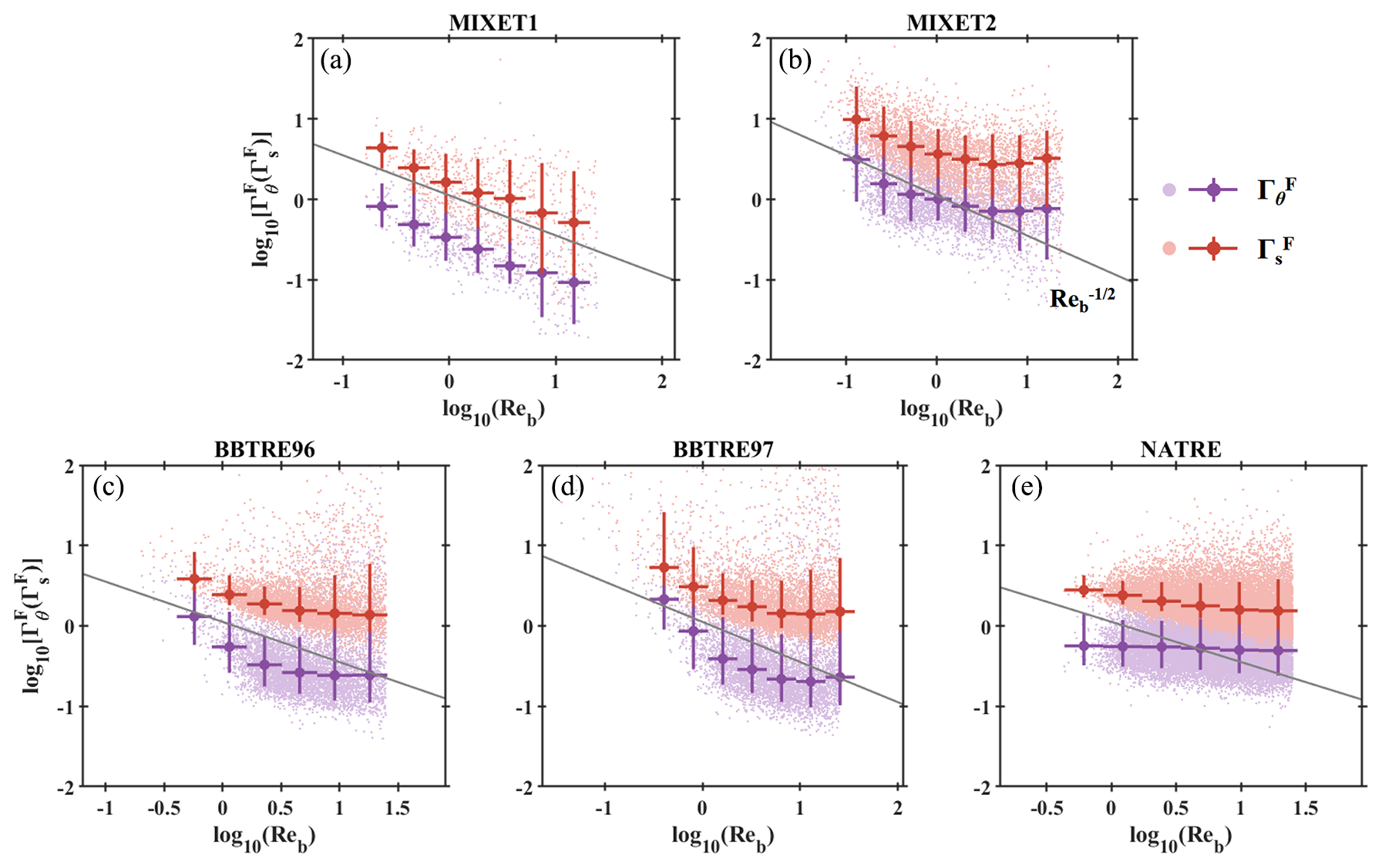
Figure 12 Relations between ${\mathrm{\Gamma }}_{\mathit{\theta }}^{\mathrm{F}}({\mathrm{\Gamma }}_{\mathrm{S}}^{\mathrm{F}}$) and Re_b for the five projects. Overlying the light-colored scatter of individual patches, the Re_b-binned median values are marked by darker large dots. The bin size and 10th–90th percentile range are denoted by the horizontal and vertical bars, respectively. The gray line in each panel marks ${\mathrm{\Gamma }}_{\mathit{\theta }}^{\mathrm{F}}\left({\mathrm{\Gamma }}_{\mathrm{S}}^{\mathrm{F}}\right)\propto R{e}_{\mathrm{b}}^{-\mathrm{1}/\mathrm{2}}$.

5 Eddy diffusivities induced by turbulence and salt fingers

5.1 Eddy diffusivities induced by turbulence

Since Γ^T deviates from the conventionally used constant of 0.2 in the Osborn relation, $K_{\mathit{\rho }}^{\mathrm{T}}$ (also $K_{\mathit{\theta }}^{\mathrm{T}}$ and $K_{\mathrm{S}}^{\mathrm{T}}$) based on Γ^T differs from K_c based on 0.2 (K_c= 0.2$\mathit{\epsilon }/N^{\mathrm{2}}$) to different extents (Fig. 13). For MIXET1, since Γ^T is only slightly larger than 0.2 in general, the magnitudes of $K_{\mathit{\rho }}^{\mathrm{T}}$ and K_c differ slightly, with mean K_c= 2.1 × 10⁻⁶ m² s⁻¹ and mean $K_{\mathit{\rho }}^{\mathrm{T}}=$ 4.6 × 10⁻⁶ m² s⁻¹. Vertically, both $K_{\mathit{\rho }}^{\mathrm{T}}$ and K_c decrease in the upper 1200 m and increase at deeper depth. Obvious differences between $K_{\mathit{\rho }}^{\mathrm{T}}$ and K_c occur at depth ranges shallower than 1200 m and deeper than 2000 m, where the mean ratios of $K_{\mathit{\rho }}^{\mathrm{T}}$ to K_c are 2.7 and 2.3, respectively. For MIXET2, the magnitude difference between $K_{\mathit{\rho }}^{\mathrm{T}}$ and K_c is larger, with the mean values being 1.3 × 10⁻⁶ and 3.9 × 10⁻⁶ m² s⁻¹, respectively. Compared with K_c that stays nearly constant in the upper 1700 m, $K_{\mathit{\rho }}^{\mathrm{T}}$ first decreases in the upper 700 m and then stays around 2 × 10⁻⁶ m² s⁻¹ between 700 and 1700 m. For BBTRE96, except for several depth bins, the difference between mean $K_{\mathit{\rho }}^{\mathrm{T}}$ and mean K_c in the upper 3700 m is small, and they share similar downward increases and similar depth-averaged median values around 2.0 × 10⁻⁵ m² s⁻¹, with $K_{\mathit{\rho }}^{\mathrm{T}}$ being about 2.5 times K_c. Although both increase at depths deeper than 3700 m, $K_{\mathit{\rho }}^{\mathrm{T}}$ is nearly 4.7 times larger than K_c, and the mean values for $K_{\mathit{\rho }}^{\mathrm{T}}$ and K_c are 5.0 × 10⁻⁴ and 1.1 × 10⁻⁴ m² s⁻¹, respectively. For BBTRE97, $K_{\mathit{\rho }}^{\mathrm{T}}$ and K_c share the same downward negative trend and magnitude in the upper 1000 m, with mean values close to 2.6 × 10⁻⁵ m² s⁻¹. Beneath 1000 m, although sharing a similar positive trend, $K_{\mathit{\rho }}^{\mathrm{T}}$ becomes larger and larger than K_c with depth. At depth between 1000 and 3700 m, $K_{\mathit{\rho }}^{\mathrm{T}}/K_{\mathrm{c}}\approx$ 2.7 with median $K_{\mathit{\rho }}^{\mathrm{T}}$ around 8.3 × 10⁻⁵ m² s⁻¹, while the corresponding values for depths deeper than 3700 m are $K_{\mathit{\rho }}^{\mathrm{T}}/K_{\mathrm{c}}\approx$8.8 and mean $K_{\mathit{\rho }}^{\mathrm{T}}\approx$ 1.2 × 10⁻³ m² s⁻¹. For NATRE, $K_{\mathit{\rho }}^{\mathrm{T}}$ is always larger than K_c at all depth ranges, and the mean values of $K_{\mathit{\rho }}^{\mathrm{T}}$ and K_c are 4.4 × 10⁻⁵ and 1.0 × 10⁻⁵ m² s⁻¹, respectively. Vertically, K_c generally fluctuates around its mean value for the whole water column. $K_{\mathit{\rho }}^{\mathrm{T}}$ also shows no clear vertical variation in the upper 2700 m, but it increases significantly from 2.6 × 10⁻⁵ m² s⁻¹ at 2700 m to 1.2 × 10⁻⁴ m² s⁻¹ at 3900 m. As a result, $K_{\mathit{\rho }}^{\mathrm{T}}$ is 13.7 times larger than K_c at 3900 m. For the five projects, taking Γ^T as a constant of 0.2 underestimates the actual eddy diffusivity induced by turbulence, and this underestimate may become more severe as Γ^T increases with depth.

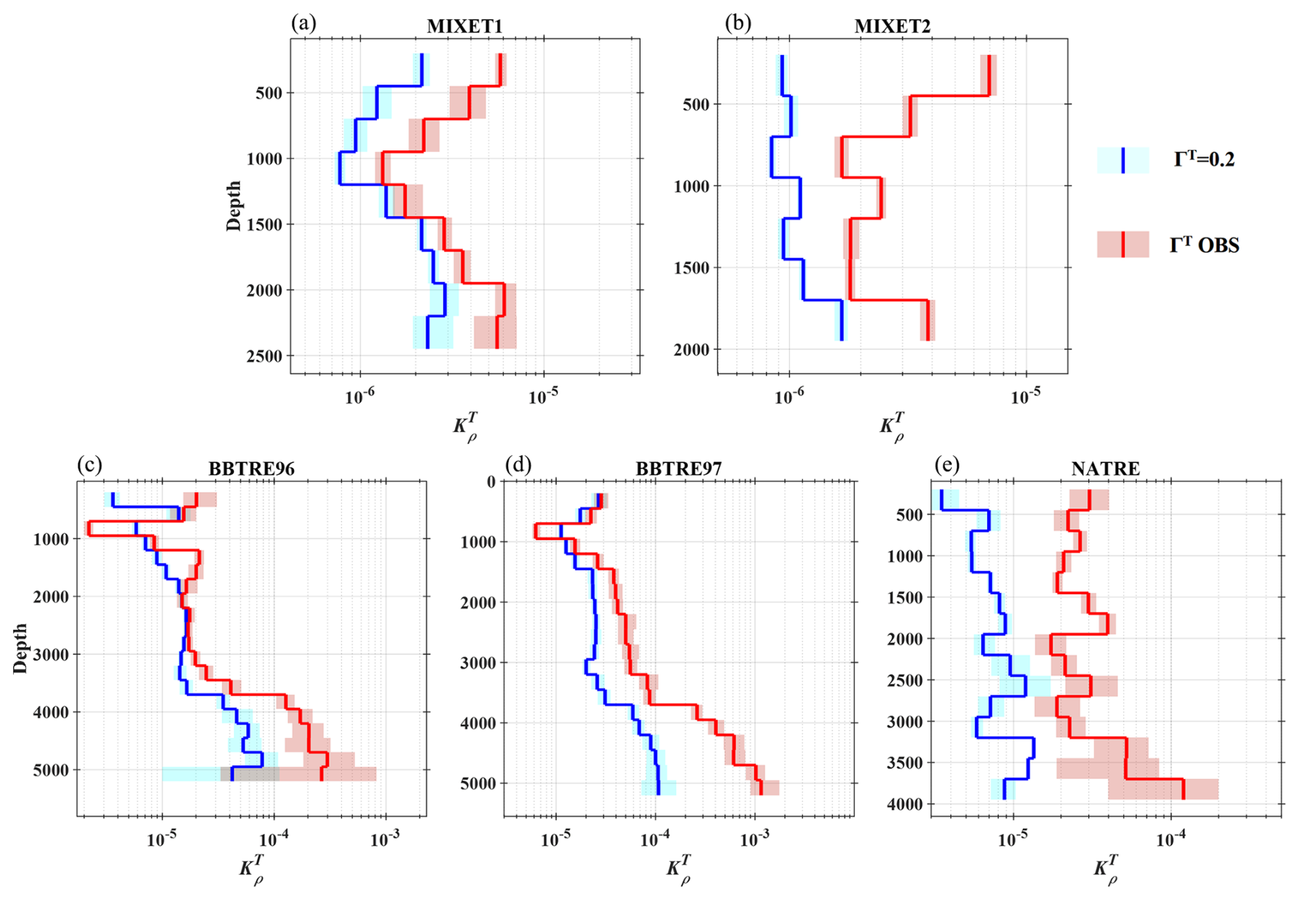
Figure 13 Vertical profiles of depth bin mean $K_{\mathit{\rho }}^{\mathrm{T}}(K_{\mathrm{c}}$) based on energetic turbulence and weak turbulence patches for the five projects. The blue curve shows K_c estimates by using Γ^T= 0.2, and the red curve shows $K_{\mathit{\rho }}^{\mathrm{T}}$ based on the measured Γ^T. The colored shading corresponds to 95 % bootstrapped confidence intervals. To exclude the influence of extreme values, we only consider patches with Γ^T between the upper and lower quartiles for each depth bin. The depth bin size is 250 m.

5.2 Eddy diffusivities induced by salt fingers

For salt-finger-induced eddy diffusivities, some studies estimated their values by taking a constant r^F of around 0.7 (0.75 in Schmitt et al., 2005; 0.6 in St. Laurent and Schmitt, 1999). Here, $K_{\mathit{\theta }}^{\mathrm{F}}$ derived from the observed r^F is compared with the r^F= 0.7 estimate, $K{}_{\mathit{\theta }\mathrm{c}}^{\mathrm{F}}$ (Fig. 14). Depending on the deviation of the observed r^F from 0.7, the five projects are distinct in terms of the difference between $K_{\mathit{\theta }}^{\mathrm{F}}$ and $K{}_{\mathit{\theta }\mathrm{c}}^{\mathrm{F}}$. For MIXET1, $K_{\mathit{\theta }}^{\mathrm{F}}$ and $K{}_{\mathit{\theta }\mathrm{c}}^{\mathrm{F}}$ both vary little with depth. But the magnitude of $K{}_{\mathit{\theta }\mathrm{c}}^{\mathrm{F}}$ is significantly greater than that of $K_{\mathit{\theta }}^{\mathrm{F}}$, with mean values being 2.2 × 10⁻⁶ and 4.6 × 10⁻⁷ m² s⁻¹, respectively. This is in line with the fact that the mean value of the measured r^F for MIXET1 is only 0.37, about one-half of 0.7. For MIXET2, with the median r^F elevated to 0.63, $K{}_{\mathit{\theta }\mathrm{c}}^{\mathrm{F}}$ is only slightly larger than $K_{\mathit{\theta }}^{\mathrm{F}}$. And they both increase with depth form O(10⁻⁶) m² s⁻¹ at 100 m to O(10⁻⁵) m² s⁻¹ at 1850 m. The median values of $K{}_{\mathit{\theta }\mathrm{c}}^{\mathrm{F}}$ and $K_{\mathit{\theta }}^{\mathrm{F}}$ are 4.4 × 10⁻⁶ and 3.2 × 10⁻⁶ m² s⁻¹, respectively. The difference between MIXET1 and MIXET2 indicates a strong seasonal variation of salt fingers in the tropical Pacific. For both BBTRE96 and BBTRE97, $K{}_{\mathit{\theta }\mathrm{c}}^{\mathrm{F}}$ is significantly larger than $K_{\mathit{\theta }}^{\mathrm{F}}$ in the upper layer with magnitudes around O(10⁻⁵) and O(10⁻⁶) m² s⁻¹, respectively, and this difference turns small as they both increase to 2 × 10⁻⁵ m² s⁻¹ with depth increasing to 2000 m. At deeper depths, although the salt finger disappears at some depth ranges, $K{}_{\mathit{\theta }\mathrm{c}}^{\mathrm{F}}$ varies little around 2.5 × 10⁻⁵ m² s⁻¹. $K_{\mathit{\theta }}^{\mathrm{F}}$ is generally larger than $K{}_{\mathit{\theta }\mathrm{c}}^{\mathrm{F}}$ between 2400 and 3400 m with $K_{\mathit{\theta }}^{\mathrm{F}}/K{}_{\mathit{\theta }\mathrm{c}}^{\mathrm{F}}$ varying between 3 and 10, and this ratio drops to less than 2 for depths deeper than 3400 m. For NATRE, both $K_{\mathit{\theta }}^{\mathrm{F}}$ and $K{}_{\mathit{\theta }\mathrm{c}}^{\mathrm{F}}$ present clear downward increases, and $K{}_{\mathit{\theta }\mathrm{c}}^{\mathrm{F}}$ is dominantly greater than $K_{\mathit{\theta }}^{\mathrm{F}}$. The difference between $K_{\mathit{\theta }}^{\mathrm{F}}$ and $K{}_{\mathit{\theta }\mathrm{c}}^{\mathrm{F}}$ is reduced with increasing depth due to the fact that $K_{\mathit{\theta }}^{\mathrm{F}}$ increases much faster with depth from about 2 × 10⁻⁶ m² s⁻¹ in the upper 500 m to 1.5 × 10⁻⁵ m² s⁻¹ at 2400 m. For all the projects, $K_{\mathit{\theta }}^{\mathrm{F}}$ is generally smaller than $K{}_{\mathit{\theta }\mathrm{c}}^{\mathrm{F}}$ since r^F is mostly smaller than 0.7, and this phenomenon is most obvious in the upper layer (upper 1000 m for BBTRE96, BBTRE97, and NATRE). At deeper depths, $K_{\mathit{\theta }}^{\mathrm{F}}$ > $K{}_{\mathit{\theta }\mathrm{c}}^{\mathrm{F}}$ can be observed in projects like BBTRE96 and BBTRE97. All of this indicates that r^F is highly variable regionally and vertically. We also explore the vertical variation of $K_{\mathrm{S}}^{\mathrm{F}}$, which is very similar to that of $K_{\mathit{\theta }}^{\mathrm{F}}$ but with a larger magnitude (Fig. 15), as a result of ${\mathrm{\Gamma }}_{\mathrm{S}}^{\mathrm{F}}$ being larger than and strongly proportional to ${\mathrm{\Gamma }}_{\mathit{\theta }}^{\mathrm{F}}$.

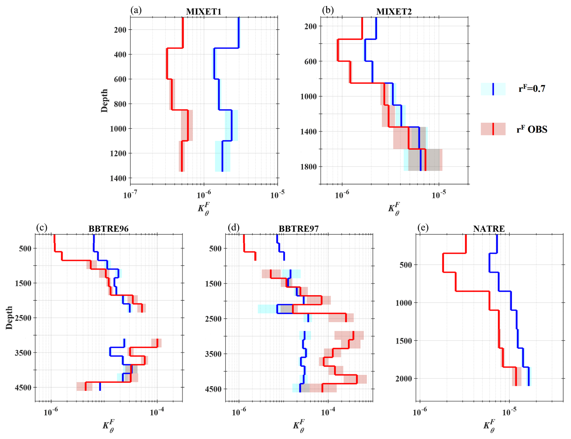
Figure 14 Vertical profiles of depth bin mean $K_{\mathit{\theta }}^{\mathrm{F}}(K{}_{\mathit{\theta }\mathrm{c}}^{\mathrm{F}}$) based on salt finger patches for the five projects. The blue curves are $K{}_{\mathit{\theta }\mathrm{c}}^{\mathrm{F}}$ estimated with r^F= 0.7, and the red ones are $K_{\mathit{\theta }}^{\mathrm{F}}$ based on the measured r^F. The colored shading corresponds to 95 % bootstrapped confidence intervals. To exclude the influence of extreme values, we only consider patches with ${\mathrm{\Gamma }}_{\mathit{\theta }}^{\mathrm{F}}$ between the upper and lower quartiles for each depth bin. The depth bin size is 250 m, and depth bins with fewer than 10 patches are excluded.

Figure 15 Same as Fig. 14, but for $K_{\mathrm{S}}^{\mathrm{F}}$.

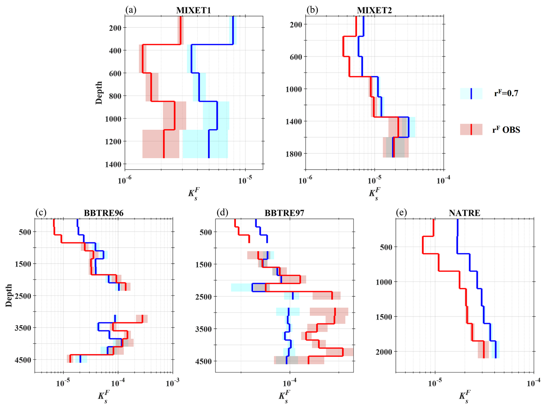
Next, we examine the vertical variation of the ratio of $K_{\mathrm{S}}^{\mathrm{F}}$ to $K_{\mathit{\theta }}^{\mathrm{F}}$ for the five projects (Fig. 16). For MIXET1, $K_{\mathrm{S}}^{\mathrm{F}}/K_{\mathit{\theta }}^{\mathrm{F}}$ generally decreases from 5.3 in the upper 400 m to 4 at 1400 m, with an averaged value of 4.5. The averaged $K_{\mathrm{S}}^{\mathrm{F}}/K_{\mathit{\theta }}^{\mathrm{F}}$ drops to 3.9 for MIXET2, and it varies between 3.7 and 4.5 except the small values shallower than 400 m and beneath 1600 m. The BBTRE projects share a similar vertical structure of $K_{\mathrm{S}}^{\mathrm{F}}/K_{\mathit{\theta }}^{\mathrm{F}}$: it has a maximum value of 6 in the upper 800 m, then sharply decreases to 2.5 at 1350 m and stays at this value until reaching 4600 m. $K_{\mathrm{S}}^{\mathrm{F}}/K_{\mathit{\theta }}^{\mathrm{F}}$ for NATRE first increases from 3.0 to 4.7 in the upper 800 m and then sharply decreases to 3 at 1100 m and remains unchanged. From the five projects, $K_{\mathrm{S}}^{\mathrm{F}}/K_{\mathit{\theta }}^{\mathrm{F}}$ generally increases with depth in the upper 1000 m with an average value about 5; then, it sharply drops to around 3 and stays at this value at deeper depths. This ratio is reported to be 2.3 in the western tropical Atlantic (Schmitt et al., 2005), slightly smaller than the result presented here. Van de Boog et al. (2021) presented a global map of $K_{\mathrm{S}}^{\mathrm{F}}$ and $K_{\mathit{\theta }}^{\mathrm{F}}$ based on Argo data and an empirical method, and their results indicate that $K_{\mathrm{S}}^{\mathrm{F}}/K_{\mathit{\theta }}^{\mathrm{F}}$ varies between 1.3 and 7.8 for R_ρ ranging from 1 to 4. These earlier works do not show the vertical variation of $K_{\mathrm{S}}^{\mathrm{F}}/K_{\mathit{\theta }}^{\mathrm{F}}$ due to indirect methods used.

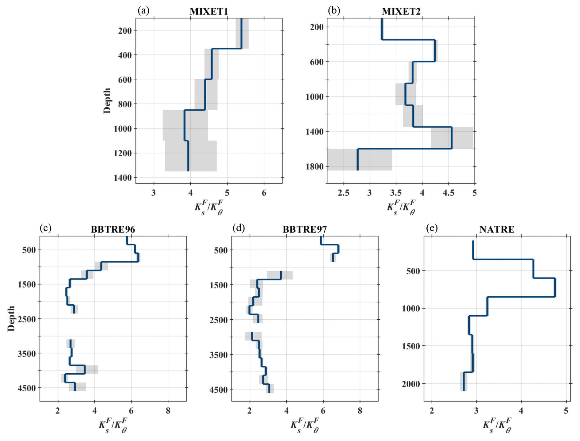
Figure 16 Vertical profiles of depth bin mean $K_{\mathrm{S}}^{\mathrm{F}}/K_{\mathit{\theta }}^{\mathrm{F}}$ based on salt finger patches for the five projects. The dark blue curves are the mean $K_{\mathrm{S}}^{\mathrm{F}}/K_{\mathit{\theta }}^{\mathrm{F}}$, and the gray shading represents 95 % bootstrapped confidence intervals. To exclude the influence of extreme values, we only consider patches with ${\mathrm{\Gamma }}_{\mathit{\theta }}^{\mathrm{F}}$ between the upper and lower quartiles for each depth bin. The depth bin size is 250 m, and depth bins with fewer than 10 patches are excluded.

5.3 “Total” eddy diffusivities under superposed salt fingers and turbulence

We examine the “total” eddy diffusivities contributed by both salt fingers and turbulence by combining the patches with weak turbulence, energetic turbulence, and salt fingers. Two different methods are used to estimate the total eddy diffusivities. The first is from McDougall and Ruddick (1992) (hereinafter MR92). MR92 does not need to differentiate salt finger and turbulent patches; it estimates the total eddy diffusivities by (i) evaluating the departure of observed Γ (Eq. 1) to a preset reasonable turbulent Γ^T (e.g., Γ^T= 0.265) and (ii) introducing a “salt flux enhancement factor”, M₀, scaled by R_ρ and r (more details are given in McDougall and Ruddick, 1992). Here, r is treated specifically depending on the mixing type – that is, r^T=R_ρ for turbulence and $r^{\mathrm{F}}=\frac{R_{\mathit{\rho }}\mathrm{\Gamma }}{R_{\mathit{\rho }}\mathrm{\Gamma }+R_{\mathit{\rho }}-\mathrm{1}}$ for salt fingers (St. Laurent and Schmitt, 1999). The second is from St. Laurent and Schmitt (1999) (hereinafter LS99), which differentiates turbulence and salt fingers first, then estimates their eddy diffusivities separately, and finally obtains the total ones as K_θ= $P^{\mathrm{T}}\cdot K_{\mathit{\theta }}^{\mathrm{T}}+P^{\mathrm{F}}\cdot K_{\mathit{\theta }}^{\mathrm{F}}$ and $K_{\mathrm{S}}=P^{\mathrm{T}}\cdot K_{\mathrm{S}}^{\mathrm{T}}+P^{\mathrm{F}}\cdot K_{\mathrm{S}}^{\mathrm{F}}$, where P^T and P^F are the number proportions of turbulence and salt finger patches to their sum, respectively. Figure 17 shows the total K_θ estimated by these two methods. Compared with BBTRE and NATRE, the results based on MR92 and LS99 present larger differences for MIXET, which may be due to fewer patches and more scattered Γ^T and Γ^F. Nonetheless, it is obvious that both estimates have a similar magnitude and vertical trend for all five projects. Comparing the total K_θ with $K_{\mathit{\theta }}^{\mathrm{T}}$ and $K_{\mathit{\theta }}^{\mathrm{F}}$ (Figs. 13, 14), we can see that K_θ, especially for the LS99 result, is obviously closer to $K_{\mathit{\theta }}^{\mathrm{T}}$ for all five projects, confirming that turbulence dominates the observed microstructures. Note that K_θ values in the upper 500 m for BBTRE and NATRE are significantly lower than $K_{\mathit{\theta }}^{\mathrm{T}}$, seemingly indicating a strong weakening of K_θ due to the prevalence of salt fingers. However, the effect of a salt finger is actually overestimated, since the dominant hybrid mixing patches at this depth range are all excluded, which should be dominated by turbulence, as indicated by the elevated Re_b. The total K_S is not shown since it is very similar to the situation of K_θ, and the only notable difference is that K_S is not significantly weakened by a salt finger in the upper 500 m for BBTRE and NATRE owing to $K_{\mathrm{S}}^{\mathrm{F}}$ being clearly greater than $K_{\mathit{\theta }}^{\mathrm{F}}$ and much closer to $K_{\mathrm{S}}^{\mathrm{T}}$ (Fig. 15).

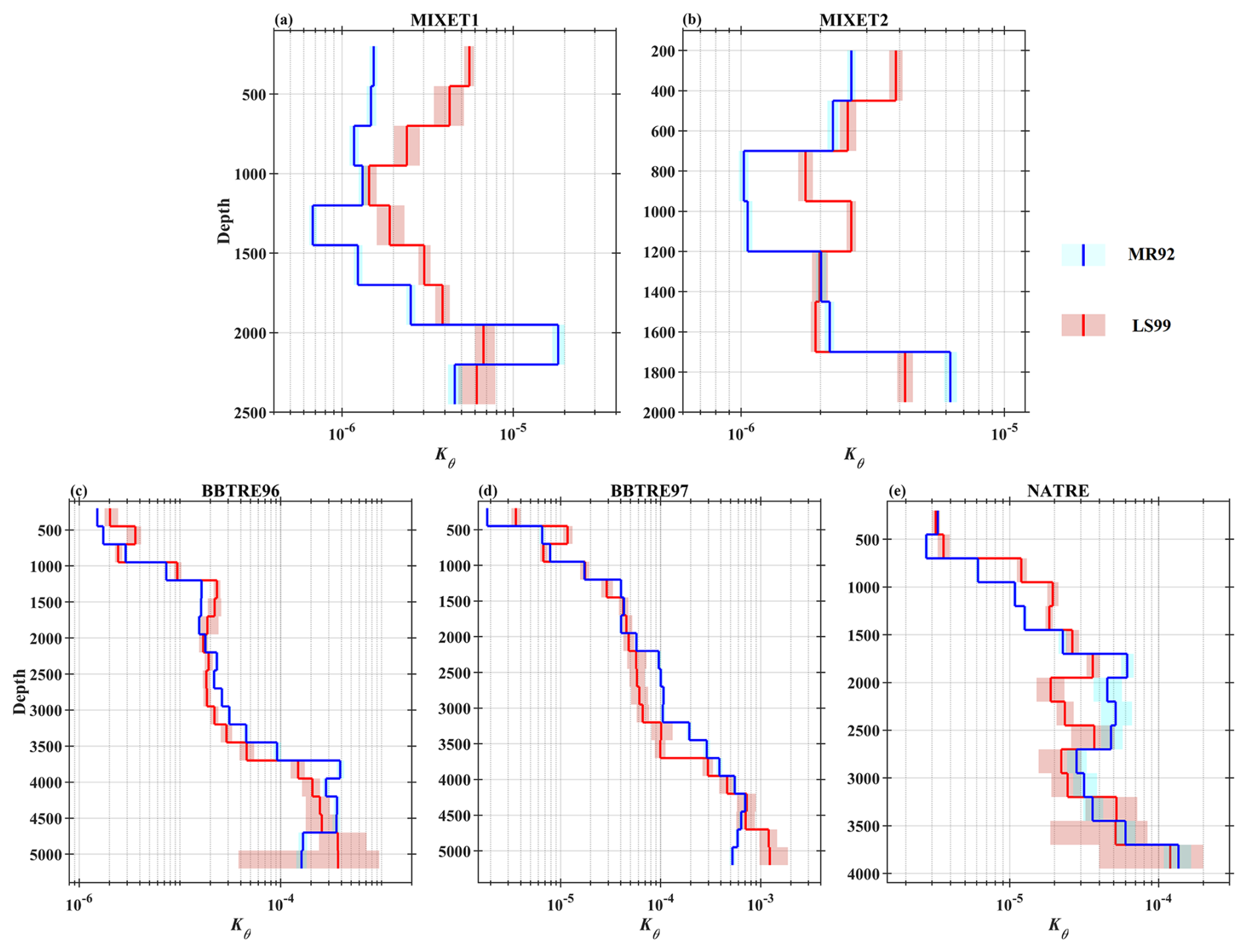
Figure 17 Vertical profiles of depth-bin-averaged total K_θ based on turbulence and salt finger patches for the five projects. The blue curves are results based on MR92, and the red ones are based on LS99. The shading corresponds to 95 % bootstrapped confidence intervals. The depth bin size is 250 m, and depth bins with fewer than 10 patches are excluded.

6 Summary

The Osborn relation is widely used to estimate vertical eddy diffusivity in practice, assuming a constant dissipation ratio of Γ^T= 0.2 without identifying the underlying mixing mechanisms. The dissipation ratios of heat, salinity, and density are equal for turbulent mixing; however, they differ for salt-finger-induced mixing. As a result, the eddy diffusivities derived from a constant dissipation ratio would inevitably depart from the actual values. In this study, we differentiated between turbulent mixing and salt finger mixing, quantified their dissipation ratios and eddy diffusivities, and examined their relations based on the datasets from the Microstructure Database.

We evaluated the variation of Γ^T and its relations to Re_b and R_OT. The observed Γ^T is scattered over orders of magnitude, typically ranging from 10⁻² to 10. The significant difference between the five projects suggests that Γ^T is highly variable with space and time. Γ^T in the western equatorial Pacific presents a weak decrease downwards, while it obviously increases in the midlatitudes in the Atlantic. Although a negative relation between Γ^T and Re_b was supported by most of the projects, further investigation of the relations of Γ^T to Re_b and R_OT suggested ${\mathrm{\Gamma }}^{\mathrm{T}}\propto R_{\mathrm{OT}}^{-\mathrm{4}/\mathrm{3}}\cdot R{e}_{\mathrm{b}}^{\mathrm{1}/\mathrm{2}}$. This indicates that Γ^T is modulated by more than one variable and explains why different relations between Γ^T and Re_b have been reported (e.g., Mashayek et al., 2017; Ijichi and Hibiya, 2018).

We compared $K_{\mathit{\rho }}^{\mathrm{T}}$ estimated using observed Γ^T with K_c estimated using Γ^T= 0.2. $K_{\mathit{\rho }}^{\mathrm{T}}$ is clearly larger than K_c. For the MIXET projects with downward weak decreasing Γ^T, $K_{\mathit{\rho }}^{\mathrm{T}}$ shares a similar vertical structure of K_c, with a magnitude elevated by about 2 or 3 times. For the rest of the projects where Γ^T increases significantly with depth, $K_{\mathit{\rho }}^{\mathrm{T}}$ generally presents a much more obvious increase than K_c, and $K_{\mathit{\rho }}^{\mathrm{T}}$ can exceed K_c by an order of magnitude. This suggests that the intensity of bottom-enhanced mixing may be underestimated when assuming Γ^T= 0.2.

For salt fingers, two effective dissipation ratios for heat (${\mathrm{\Gamma }}_{\mathit{\theta }}^{\mathrm{F}}$) and salt (${\mathrm{\Gamma }}_{\mathrm{S}}^{\mathrm{F}}$) are derived, and two artificial Osborn relations are used to calculate the corresponding eddy diffusivities. ${\mathrm{\Gamma }}_{\mathit{\theta }}^{\mathrm{F}}$ spans about 2 orders of magnitude. Both the magnitude and vertical structure of ${\mathrm{\Gamma }}_{\mathit{\theta }}^{\mathrm{F}}$ are distinct for the five projects. ${\mathrm{\Gamma }}_{\mathrm{S}}^{\mathrm{F}}$ is strongly related to ${\mathrm{\Gamma }}_{\mathit{\theta }}^{\mathrm{F}}$, and they exhibit similar vertical structures, ${\mathrm{\Gamma }}_{\mathrm{S}}^{\mathrm{F}}\approx$ 5 ${\mathrm{\Gamma }}_{\mathit{\theta }}^{\mathrm{F}}$. Data from some projects indicate a negative relation between ${\mathrm{\Gamma }}_{\mathit{\theta }}^{\mathrm{F}}$ (${\mathrm{\Gamma }}_{\mathrm{S}}^{\mathrm{F}}$) and Re_b, while others suggest no clear relation. Unlike the existing results indicating that r^F decreases and then asymptotes to a constant value with increasing R_ρ, our results suggest that r^F decreases sharply with R_ρ when it is smaller than 2.4 and grows to a larger value with R_ρ when it exceeds 2.4.

We examined salt-finger-induced $K_{\mathit{\theta }}^{\mathrm{F}}$ and $K_{\mathrm{S}}^{\mathrm{F}}$. Although a salt finger becomes rarer with depth, $K_{\mathit{\theta }}^{\mathrm{F}}$ and $K_{\mathrm{S}}^{\mathrm{F}}$ increase clearly with depth, and $K_{\mathrm{S}}^{\mathrm{F}}$ is greater than $K_{\mathit{\theta }}^{\mathrm{F}}$. In the upper 1000 m, $K_{\mathrm{S}}^{\mathrm{F}}$ is significantly greater than $K_{\mathit{\theta }}^{\mathrm{F}}$ by about 5 times for most projects, but below 1000 m, $K_{\mathrm{S}}^{\mathrm{F}}/K_{\mathit{\theta }}^{\mathrm{F}}$ generally remains around 3. $K_{\mathit{\theta }}^{\mathrm{F}}$ and $K_{\mathrm{S}}^{\mathrm{F}}$ estimated using the observed r^F are generally smaller than those using r^F= 0.7 due to most observed r^F values being smaller than 0.7 but varying more sharply with depth.

Compared with eddy diffusivity induced by turbulence, $K_{\mathit{\theta }}^{\mathrm{F}}$ is smaller than $K_{\mathit{\theta }}^{\mathrm{T}}$ in the upper 1000 m, but they become increasingly comparable with depth. $K_{\mathrm{S}}^{\mathrm{F}}$ is close to or even larger than $K_{\mathrm{S}}^{\mathrm{T}}$ at all depths for all the projects. In general, although salt finger events are much rarer than turbulence at depth (so they are incapable of significantly altering the background mixing intensity shaped by turbulence), they can play a crucial role in local, short-period mixing events, which is worth investigating and properly parameterizing in numerical models.