Decadal changes in phytoplankton functional composition in the Eastern English Channel: possible upcoming major effects of climate change

Global change is known to exert a considerable impact on marine and coastal ecosystems, affecting various parameters such as sea surface temperature (SST), runoff, circulation patterns and the availability of limiting nutrients (like nitrogen, phosphorus and silicon), with each influencing phytoplankton communities differently. This study is based on weekly to fortnightly in vivo fine-spatial-resolution (∼ 1 km) phytoplankton observations along an nearshore–offshore gradient in the French waters of the Eastern English Channel in the Strait of Dover. The phytoplankton functional composition was addressed by automated “pulse-shape recording” flow cytometry, coupled with the analysis of environmental variables over the last decade (2012–2022). This method allows for the characterization of almost the entire phytoplankton size range (from 0.1 to 800 µm width) and the determination of the abundance of functional groups based on optical single-cell signals (fluorescence and scatter). We explored seasonal, spatial and decadal dynamics in an environment strongly influenced by tides and currents. Over the past 11 years, the SST has shown an increasing trend at all stations, with nearshore waters warming faster than offshore waters (+1.05 °C vs. +0.93 °C). Changes in nutrient concentrations have led to imbalances in nutrient ratios ($\mathrm{N}:\mathrm{P}:\mathrm{Si}$) relative to reference nutrient ratios. However, a return to balanced ratios has been observed since 2019. The phytoplankton total abundance has also increased over the aforementioned decade, with a higher contribution of small-sized cells (picoeukaryotes and picocyanobacteria) and a decrease in microphytoplankton, particularly near the coast. Based on an analysis of environmental parameters and phytoplankton abundance, the winters of 2013–2014 and 2019–2020 were identified as shifting periods in this time series. These changes in the phytoplankton community, favoring the smallest groups, could lead to a reduction in the productivity of coastal marine ecosystems, which could, in turn, affect higher trophic levels and the entire food web.

1 Introduction

As the main primary producer of marine ecosystems, marine phytoplankton play a crucial role in structuring pelagic food webs and greatly influence biogeochemical cycles in the ocean. This polyphyletic group exhibits a wide range of sizes (from less than 1 µm to centimeters), shapes, single-cell or colonial forms, life stages, pigments, storage products, motility, and reproductive rates, among others (Simon et al., 2009). All of these functional traits, especially size, will determine their involvement and performance in biogeochemical cycling (e.g., carbon fixation and nutrient uptake; Hillebrand et al., 2022), their growth rate (Marañón, 2015) and their energy transfer efficiency to higher trophic levels (Mehner et al., 2018). The abundance, the community composition and the succession of different phytoplankton groups are rapidly regulated by environmental parameters (sea surface temperature, light availability and nutrient availability) and biotic interactions (Margalef, 1978; Winder and Sommer, 2012; Barton et al., 2013; Rombouts et al., 2019). Due to the rapid turnover between generations and the response of communities to environmental changes, phytoplankton are used as an indicator to assess the ecological status of pelagic marine ecosystems. In the context of the Marine Strategy Framework Directive (MSFD, 2008/56/EC), phytoplankton diversity, composition and abundance are used to assess the ecological status of pelagic habitats (Louchart et al., 2023a, b; Holland et al., 2023a) and to study marine eutrophication (Rombouts et al., 2019).

In addition to local pressures, climate change significantly influences environmental parameters in marine systems, leading to rising sea surface temperatures (SSTs), changes in light intensity, and changes in rainfall and river flow (Cooley et al., 2022). Coastal and shallow environments are particularly vulnerable to these changes (Cloern et al., 2016). While these global-scale modifications have already been observed at regional levels, they have not yet been observed at the sub-mesoscale (Capuzzo et al., 2018).

The Eastern English Channel (EEC) is a shallow marginal sea under a macrotidal regime that experiences a large anthropogenic influence. It is an exploited ecosystem with respect to fisheries, hosting major harbors such as Cherbourg, Le Havre, Boulogne-sur-Mer and Calais along the French coast. The EEC is also subjected to intense maritime traffic, particularly in the Strait of Dover, which connects the English Channel to the North Sea and ranks as the world's second-busiest strait. Furthermore, the coastline is largely covered by agricultural land, leading to potential nutrient and/or pesticide inputs into coastal waters through rainfall and runoff. In addition, the EEC coast is characterized by numerous estuaries, including the Seine, the Somme and smaller estuaries (the Authie, Canche, Liane, Wimereux and Slack), terminating in the Strait of Dover; these waterways collectively contribute to the “coastal flow” and generate significant terrigenous inputs (Brylinski et al., 1991). Over the last 150 years, the English Channel has witnessed a rise in precipitation (Scholz et al., 2022); moreover, a notable increase in SST has been observed in the Eastern English Channel since the 1990s (McLean et al., 2019; Tinker et al., 2020). Furthermore, changes in nutrient concentrations have been observed since the implementation of the European common agricultural policy (CAP), resulting in a stronger phosphorus mitigation effort compared with nitrogen and leading to an imbalanced N:P ratio (Loebl et al., 2009; Talarmin et al., 2016; Lheureux et al., 2023). These modifications are expected to have consequences for phytoplankton communities in the EEC, affecting their abundance, composition, size and bloom timing (Falkowski and Oliver, 2007; Sommer and Lengfellner, 2008; Winder and Sommer, 2012; Henson et al., 2018; Rombouts et al., 2019).

Previous time-series studies have revealed a decline in phytoplankton biomass in the EEC using chlorophyll-a measurements (Lefebvre et al., 2011; Gohin et al., 2019). Over the past decade, analysis of Continuous Plankton Recorder (CPR) data has shown a change in the phytoplankton composition in the North Sea, characterized by an increase in diatoms and dinoflagellates (Holland et al., 2023b). In the EEC, the years between 1992 and 2007 could be categorized according to the dominance of the haptophyte Phaeocystis globosa or diatoms (Lefebvre et al., 2011). Previous long-term studies in the EEC, based on satellite images, chlorophyll a, microscopy or CPR data, enable one to address some changes in phytoplankton phenology and diversity, but they neglect picophytoplankton and some nanophytoplankton. In the Western English Channel, it has been shown that small phytoplankton represented 99.98 % and 71 % of the respective phytoplankton abundance and biomass (McQuatters-Gollop et al., 2024) and that an SST increase can lead to changes in the structure and cell size of this community (Zohary et al., 2021). However, these compartments have been overlooked by microscope observations, although they play a significant role in marine ecosystems by recycling nutrients and dissolved organic matter (the microbial loop) and exporting carbon to higher trophic levels via zooplankton consumption. In a context of climate change, a modification to the balance between the pico- and nanophytoplankton community structure could increase the importance of the microbial loop and microbial food webs; reduce carbon sequestration (respiration, carbon fixation and ocean carbon export); change the trophic pathways; and, in summary, influence higher trophic levels, including fisheries (Falkowski et al., 2000; Laws et al., 2000; Hillebrand et al., 2022).

In this study, we used data acquired regularly since 2012 on the full size range of phytoplankton, including picophytoplankton, addressed in vivo by automated “pulse-shape recording” flow cytometry, coupled with environmental variables. Some previous studies applying this approach in the EEC have been performed and describe seasonal changes (Bonato et al., 2016), short interannual changes (Breton et al., 2017), and spatial and temporal variability during oceanographic cruises (Bonato et al., 2015; Louchart et al., 2020, 2024). The aim of this study was to identify and quantify changes at the sub-mesoscale and to report (for the first time) decadal trends in the entire phytoplankton community. The approach combines relatively high-frequency sampling with high spatial resolution, complementing most reference observation networks for all types of water, from inshore to offshore, in a frontal system near the Strait of Dover. To characterize these trends and assess the magnitude of the change in phytoplankton communities over a decade, we applied a functional community composition approach. This approach considered temporal changes in biomass, abundance and composition, relative to changes in environmental variables, from the single-cell level up to the community level.

2 Materials and methods

2.1 Study area and sampling strategy

Subsurface marine samples were collected weekly to fortnightly, from February 2012 to December 2022, aboard the R/V Sepia II (CNRS INSU-FOF, Centre National de la Recherche Scientifique Institut National des Sciences de l’Univers – Flotte Océanographique Française). The dataset consists of 1835 samples distributed along a longitudinal transect that were collected over 268 sampling dates. Sampling was conducted along a nearshore–offshore monitoring transect by the Strait of Dover (EEC), known as the DYPHYRAD (DYnamics of PHYtoplankton on RADiale of the Saint-Jean Bay) transect. This transect consists of nine sampling stations (Fig. 1), from R0 (50°8^′ N, 1°59^′ E) to R4 (50°8^′ N, $\mathrm{1}\mathrm{°}{\mathrm{45}}^{\prime }{\mathrm{22}}^{\prime \prime }$ E), that are spaced at a distance of between 0.8 and 1.7 km from one another. The stations characterize the following three zones (from offshore to nearshore), in order to facilitate the description of spatial phenomena, according to Brylinski et al. (1991): offshore (R4, R3 and R3^′), frontal (R2 and R1^′) and nearshore (R1, R0^′ and R0).

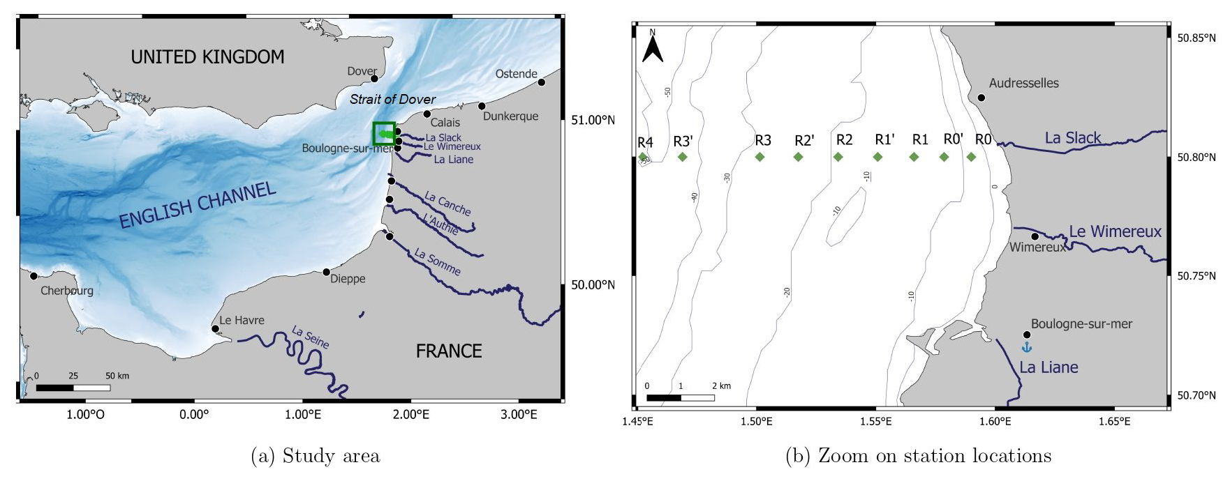
Figure 1 Map of the study area showing (a) the Eastern English Channel and (b) the location of the DYPHYRAD stations off the Slack River estuary by the Strait of Dover.

2.2 Environmental parameters

The subsurface (1–2 m depth) sea surface temperature (SST, °C) and salinity (S, PSU) were recorded at each sampling station with a conductivity–temperature–depth (CTD) probe (SBE 19plus and SBE 25, Sea-Bird Scientific, USA). Subsurface water layer (1 m depth) samples were collected using a Niskin bottle. Dissolved inorganic nutrient (${\mathrm{NO}}_{\mathrm{2}}^{-}$, ${\mathrm{NO}}_{\mathrm{3}}^{-}$, Si(OH)₄ and H₃PO₄) concentrations were measured at the main sampling points (R0, R1, R2, R3 and R4). Seawater samples were collected, kept cool and in the dark by placing them in an icebox with ice packs for up to 3 h until return to the laboratory, and were then frozen (−20 °C) upon arrival at the laboratory until analysis. This nutrient preservation process is recommended when samples cannot be analyzed on the same day (Aminot and Kérouel, 2007). Nutrient concentrations were obtained using an autoanalyzer (an Alliance Integral Futura, Italy, before 2016 and an AA3 HR AutoAnalyzer, SEAL Analytical GmbH, Germany, since 2016), following the French coastal observation network “Service d'Observation en Milieu Littoral” (SOMLIT) protocol (Garcia and Oriol, 2019; Breton et al., 2023).

2.3 Phytoplankton biomass, abundance and size

Phytoplankton biomass was approached using chlorophyll-a concentration analysis in subsurface waters, even though we acknowledge that there is a variability in the Chl:C ratio. Between 250 mL and 1 L of seawater was filtered on 47 mm diameter GF/F (Whatman) filters and then stored at −80 °C until pigment analysis, after extraction using 90 % acetone at 4 °C overnight. Chlorophyll-a and degraded-pigment (phaeopigments) concentrations were measured both before and after acidification (with HCl at 0.2 mol L⁻¹) using a Turner Designs benchtop fluorometer (10-AU field fluorometer, Turner Designs Ltd, USA), following the protocol developed by Holm-Hansen et al. (1965) and the equations developed by Lorenzen (1967).

Phytoplankton functional composition was obtained from in vivo samples using CytoSense cytometers (CytoBuoy b.v., the Netherlands). Over the 11 years of the time series, four cytometers were used. To ensure maximum comparability between the data from each instrument, the data were acquired using, to the degree possible, the same protocols and were then processed by the same person to maintain clustering consistency. In addition, only abundances were used, to avoid the risk of biasing the analysis by the inclusion of fluorescence measurements that were highly machine dependent. Abundances were compared on common samples when machines were changed. The flow cytometers are equipped with a blue laser (488 nm, 50 mW) to allow discrimination between phototrophic and non-phototrophic particles. Flow cytometers provide the counting of particle for sizes from 0.1 to 800 µm width, to consider practically the whole phytoplankton size range. The technical specifications for the flow cytometer utilized can be found in previous studies using this instrument at the Laboratory of Oceanology and Geosciences (LOG; Bonato et al., 2015, 2016; Louchart et al., 2024). Each sample underwent analysis using two separate protocols, each targeting specific size and optical parameters. The first protocol, referred to as the “Pico” protocol, used a low detection threshold (around 10 mV for red fluorescence), a low pump speed (5 µL s⁻¹) and a short sampling time (5 min). This protocol targeted cells ranging from 0.1 to 3 µm in size, characterized by low fluorescence and high abundance. The second protocol focused on nano- and microphytoplankton, using a higher detection threshold (around 25 mV for red fluorescence), a high pump speed (between 10 and 13 µL s⁻¹) and a long sampling time (8–10 min).

Manual discrimination and characterization of six main phytoplankton functional groups (PFGs) were performed on the basis of their size distribution, structure complexity and fluorescence signals, in accordance with the interoperable vocabulary of Thyssen et al. (2022). Cytogram analysis (a biplot combining scatters or fluorescence) was performed using the CytoClus 4 software (CytoBuoy b.v., the Netherlands). Several of these functional groups have previously been identified in the area, including OraPicoProk (e.g., cells of Synechococcus spp.), RedPico (e.g., picophytoplankton), RedNano (e.g., nanophytoplankton, mainly dominated by Phaeocystis globosa during the spring bloom; Bonato et al., 2015, 2016; Guiselin, 2010), HsNano (e.g., coccolithophore-type cells), OraNano (e.g., cryptophyte-type cells) and RedMicro for microphytoplankton (Fig. 2).

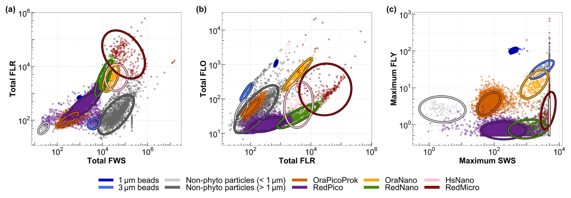
Figure 2 Cytograms of the EEC used to characterize the main phytoplankton groups: (a) total red fluorescence vs. total forward scatter for the discrimination of picoeukaryotes (RedPico), nanoeukaryotes (RedNano) and microeukaryotes (Red Micro); (b) total red fluorescence vs. total orange fluorescence for the discrimination of Synechococcus spp. (OraPicoProk) and cryptophytes (OraNano); and (c) maximum yellow fluorescence vs. maximum sideward scatter for the discrimination of the coccolithophores (HsNano). Ellipses on the graphs are calculated from a t distribution at a 95 % confidence level and aid with the accurate delineation of the respective phytoplankton groups.

For the final PFG dataset, only picoeukaryotes (RedPico) and cyanobacteria (OraPicoProk) were considered in the “Pico” protocol. The other groups (RedNano, OraNano, HsNano and RedMicro) were classified using the “Micro” protocol. To accurately perform PFG discrimination and labeling, we used 1 and 3 µm fluorescent beads, labeled with yellow and multi-fluorescence dyes using FluoSpheres carboxylate-modified microspheres (invitrogen, 1.0 µm, yellow–green fluorescent) and Sphero beads (Spherotech Inc., 3.0–3.4 µm, bright intensity), respectively.

2.4 Statistical analysis

All data analysis, graphical representations and statistical analyses were carried out using R software (R Project, CRAN), version 4.3.1. The plots were produced using the “ggplot2” package, version 3.5.0. Date management was implemented using the “lubridate” package, version 1.9.3. Multivariate statistical analyses were performed using the “vegan” package, version 2.6-4, and trend tests were performed using the “trend” package, version 1.1.6.

2.4.1 Spatial and seasonal pattern

Spatial and annual variabilities in the environmental parameters and phytoplankton communities were investigated along the DYPHYRAD transect. Stations were not uniformly sampled due to difficult weather conditions. Thus, we applied a linear time-series interpolation at each station to fill these gaps and define regular and complete sampling intervals. The abundance data were log ₁₀+1 transformed in order to reduce the weight of high abundance in the analyses. Seasonal dynamics was evaluated by applying a generalized additive model (GAM). This statistical model develops linear regression by considering nonlinear relationships between dependent and independent variables through the use of smoothing functions. In this study, the GAM facilitated the exploration of variability in PFG abundance over time using smooth spline estimation, as shown in the following formula:

$$\begin{array}{}\text{(1)}& g\left(\text{abundance}\right)=S_{\mathrm{0}}+S\left(\text{year}\right)+\mathit{ϵ},\mathit{ϵ}N(\mathrm{0},{\mathit{\sigma }}^{\mathrm{2}}),\end{array}$$

where S₀ is the intercept, S is the smoothing function, ϵ is the GAM regression and σ is the standard deviation.

This method facilitates the modeling of nonlinear relationships between the time factor and the abundance variable. We applied these GAMs individually to each PFG within every station. These relationships were created using the mgcv GAM function, without any manually imposed constraints. The smoothing of the curves corresponds to the smoothing of the GAM function in the “Smoothed conditional means” package.

2.4.2 Spatiotemporal interaction

To assess the spatiotemporal variability in PFGs over the different years, seasons and stations included in the time series, we used PERmutational Multivariate ANalysis Of VAriance (PERMANOVA). This statistical method is particularly robust because it is nonparametric and relies on permutations in the context of the Bray–Curtis distance matrix that was used. Before conducting the analysis, we standardized the abundance values using a Hellinger transformation, as proposed by Legendre and Gallagher (2001), to reduce the influence of the most dominant groups while also preserving the contribution of rare groups. This standardization is often applied to abundance data, as it preserves the proportions between groups while also reducing the effect of the extreme values maintaining the distances between samples. The strength of PERMANOVA lies in its permutation-based testing approach, making it resilient against assumptions about the data distribution. In this study, we performed 999 permutations to ensure the robustness and statistical validity of the results. In the event of a significant difference within a parameter (year, season or station), a post hoc Tukey multiple-comparison test (or Tukey's honestly significant difference) was performed (Tukey, 1949) to determine which of the possible pairs had a significant difference at a 95 % confidence interval.

2.4.3 Decadal changes and trends

The analysis of decadal changes and trends in time series was based on the processing of raw data, which were averaged on a monthly basis to establish a consistent and regular time interval. To analyze changes without eliminating the seasonal cycle, we subtracted the monthly average for each year from the monthly average for the entire period under consideration.

The cumulative sums method was used to analyze trends and patterns in the time-series dataset after checking the non-normality of the data with a Shapiro–Wilk test (Shapiro and Wilk, 1965). This method is particularly robust in the case of data series with gaps, noise or a non-normal distribution (Regier et al., 2019). The cumulative sums corresponded to the successive addition of each anomaly value in chronological order. By analyzing these cumulative sums over time, we were able to define periods of below-average values (in the case of a decreasing slope) and above-average values (in the opposite case of an increasing slope; Regier et al., 2019) and deduce phases of increasing or decreasing parameters of interest. Moreover, a change in the direction of the slope can be used to identify inflection points in the series (Regier et al., 2019).

The Mann–Kendall trend test was applied to determine the general direction of trends over time (monotonic trend; Mann, 1945; Kendall, 1948) to obtain the general sign of the slope (by summing all the signs two by two) for each parameter. The Mann–Kendall test gives no indication of the magnitude of the trend, only its sign. This was combined with a Sen slope calculation to quantify the magnitude of change within the series (Sen, 1968). This nonparametric test was used to obtain a slope value corresponding to the median of all slopes (expressed in units per decade) in the series (in pairs). These trend tests were carried out on the whole series, analyzing trends by station in order to observe small-scale spatial variations.

2.4.4 Nutrient stoichiometry

Potential nutrient limitations over the last decade were identified using a diagram of $\mathrm{Si}:\mathrm{N}:\mathrm{P}$ molar ratios where data were averaged by year. This diagram is based on the ratios Si:N $=\mathrm{1}:\mathrm{1}$, N:P $=\mathrm{16}:\mathrm{1}$ and Si:P $=\mathrm{16}:\mathrm{1}$ previously described by Redfield et al. (1963) and Brzezinski (1985). To improve visualization, the axes were transformed into a log ₁₀ scale and the graph was divided into six zones, each describing a nutrient limitation, as was previously done by Pannard et al. (2008), Schapira et al. (2008) and Akanmu (2018).

3 Results

3.1 Seasonal pattern along a nearshore–offshore gradient

The generalized additive model (GAM) modeling environmental parameters offered valuable insights into the characteristics of transect dynamics throughout a standard year (Fig. 3). The SST peaked between day 220 and day 240 (Julian day), depending on the station, preceded by minimum values between day 30 and day 60 of the year. Spatial fluctuations in SST were nuanced, with slight shifts between increases and decreases. In particular, nearshore waters showed greater reactivity than offshore waters, with an SST that was colder in winter and warmer in summer, earlier than in offshore waters. Salinity was highest in summer, showing a gradual increase from winter values and an abrupt decrease during the summer–autumn transition. Salinity revealed a distinct and contrasting spatial pattern between nearshore and offshore waters, with station R0 consistently displaying lower salinity levels (from 33.10 to 34.10) compared with others stations along the transect. Salinity levels increased progressively from coastal waters towards offshore waters, punctuated by intermittent periods of inversion, such as those observed between day 1 and day 70 (11 March) at station R4, where salinity fell below that of R3^′. The spatial difference was less marked in summer compared with winter. Nutrient concentrations also showed a seasonal pattern, starting with high values during the first months of the year (January–February), followed by a decline in spring, before increasing again from summer to autumn–winter. Silicic acid (dissolved Si) showed a sharp depletion from offshore to nearshore waters, with lower concentrations around day 110 (from 0.3 to 0.6 µmol L⁻¹) and a notable early increase observed at station R0 around day 200 (19 July) compared with a later increase at the other stations. Dissolved phosphate (dissolved P) and [${\mathrm{NO}}_{\mathrm{2}}^{-}$ + ${\mathrm{NO}}_{\mathrm{3}}^{-}$] concentrations showed similar temporal dynamics, both declining in spring, later than the dissolved Si concentration, following different trends at nearshore stations. The [${\mathrm{NO}}_{\mathrm{2}}^{-}$ + ${\mathrm{NO}}_{\mathrm{3}}^{-}$] concentration increased from offshore to nearshore areas and was almost depleted in late-spring and summer, whereas R0 showed an slightly earlier summer–autumn increase compared with offshore waters. Dissolved P showed a more complex pattern, with a higher dissolved P concentration at the nearshore R0 station in spring and an increase from day 155, earlier than the rest of the stations (increase registered from day 180 to 220).

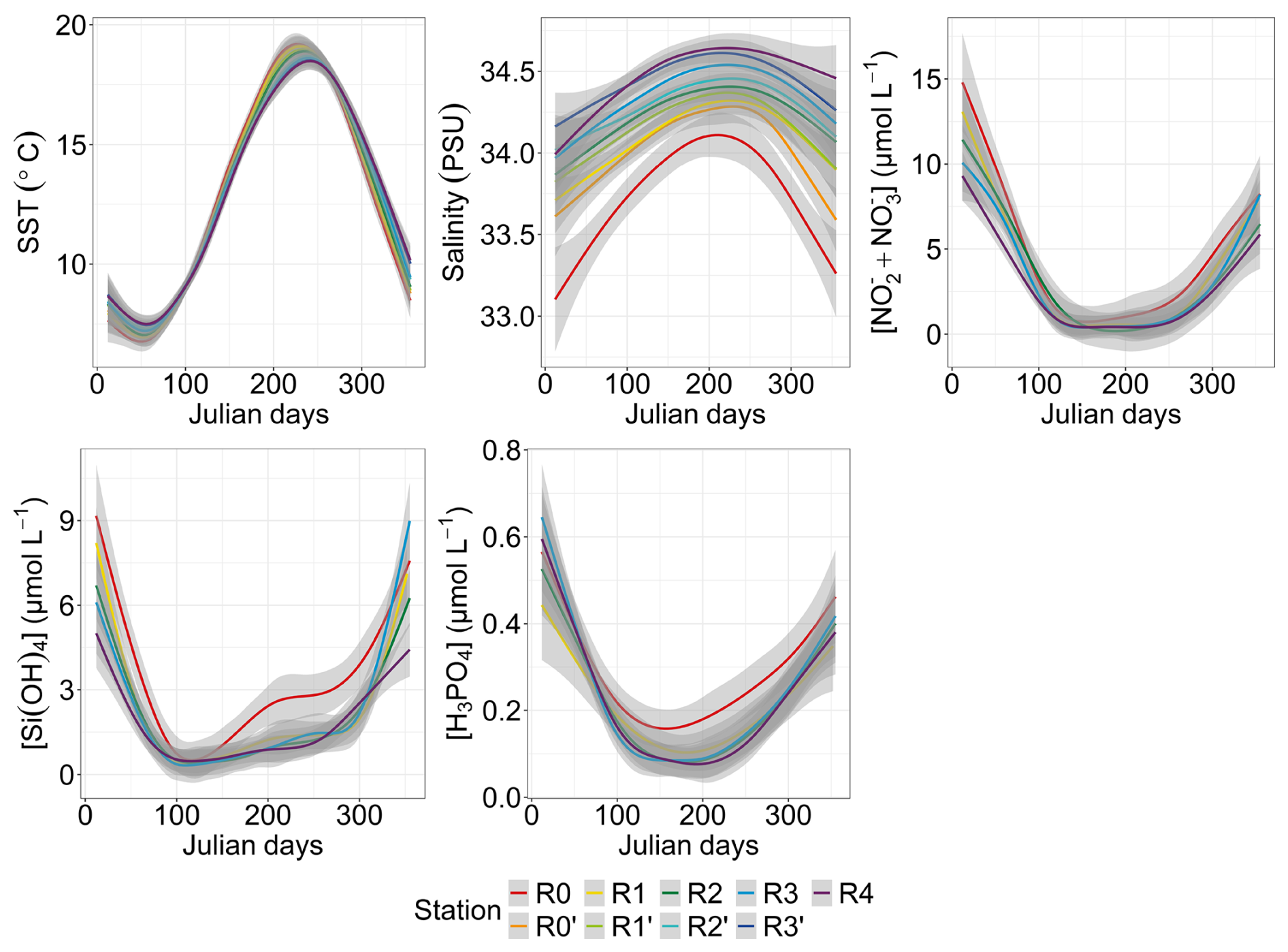
Figure 3 Seasonal and spatial variability in environmental parameters: SST (N=1766), salinity (N=1729), [${\mathrm{NO}}_{\mathrm{2}}^{-}$ + ${\mathrm{NO}}_{\mathrm{3}}^{-}$] (N=1021), dissolved Si (N=1017) and dissolved P (N=1024). The smoothed curves are modeled per Julian day using a GAM. The shaded area is the confidence interval.

The chlorophyll-a concentration showed a pronounced increase early in the year, reaching higher values (3–7.5 µg L⁻¹ during the spring bloom) from day 85 to day 95 at all stations (more particularly at station R0^′), followed by a decrease to values similar to stations R0, R1 and R1^′ (Fig. 4a). A strong spatial gradient was evident when grouping the first four nearshore stations, the two frontal stations (R2 and R2^′) and the three offshore stations (R3, R3^′ and R4). This was much more pronounced during the bloom period than during the rest of the year, with the concentration at the most coastal station (R0) decreasing to offshore levels from late spring. On the other hand, total abundance showed a pattern opposite to that of chlorophyll a, with a minimum abundance in spring and a maximum in summer (Fig. 4b). An increase in total abundance was evidenced from spring only at the two nearshore stations R0 and R0^′, whereas a marked spatial pattern was observed from late-spring and summer to early autumn, with decreasing abundance from offshore waters (R4, R3 and R3^′) to the frontal area (R2^′, R2 and R1^′), reaching the lowest cell abundance in nearshore waters (R1, R0^′ and R0).

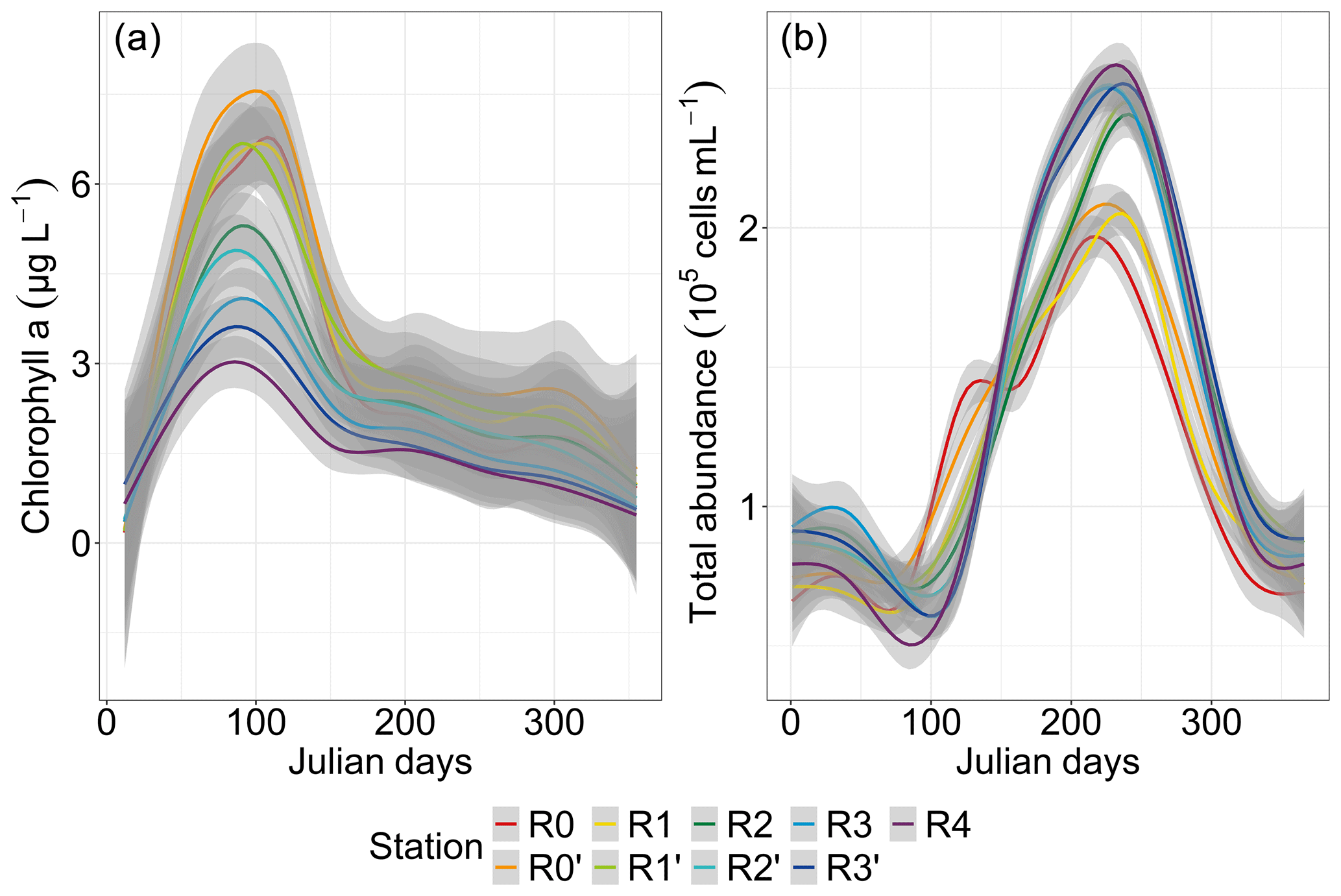
Figure 4 Seasonal and spatial variability in total phytoplankton parameters: chlorophyll a (N=1769) and total abundance (N=1522 and N interpolated = 35 712). The smoothed curves are modeled per Julian day using a GAM. The shaded area is the confidence interval.

The GAM analysis revealed a relatively high variability across space and over time for the six PFGs (Fig. 5). The seasonal heterogeneity was most striking across the PFGs, rather than across different water bodies for a single PFG. However, RedMicro and HsNano (as well as, to a lesser extent, RedNano in spring) presented a marked spatial heterogeneity. PFGs with phycobilin dominance (OraPicoProk and OraNano) reached their lowest abundance in spring (April–May) and their highest abundance during the summer–early-autumn period (July–September). The abundance of these PFGs increased along the nearshore–offshore transect. On the other hand, the abundance of PFGs with chlorophyll-a dominance (RedPico, RedNano, RedMicro and HsNano) decreased along the nearshore–offshore transect. The seasonal pattern in RedPico followed those in OraPicoProk and OraNano. The seasonality of RedNano was characterized by the highest abundance in spring (April–May) and the lowest abundance in summer, with minimum values in autumn–winter. Throughout the rise and fall of the spring bloom, the RedNano group displayed almost no apparent spatial dynamics, although there was some spatial difference when considering their total abundances. During the autumn–winter period, the nearshore–offshore pattern of RedNano disappeared and was replaced by a different spatialization, with a higher abundance in the middle of the transect and lower abundances at the extreme stations (R0 and R4). RedMicro abundance increased from January to July before dropping. Towards the end of the year (from day 250), RedMicro abundance was the highest at the R0^′ and R1^′ stations. HsNano abundance was more variable than that of any other PFG, maybe because of the low occurrence of highly scattering PFG in the study area (coccolithophores and thecate dinoflagellates).

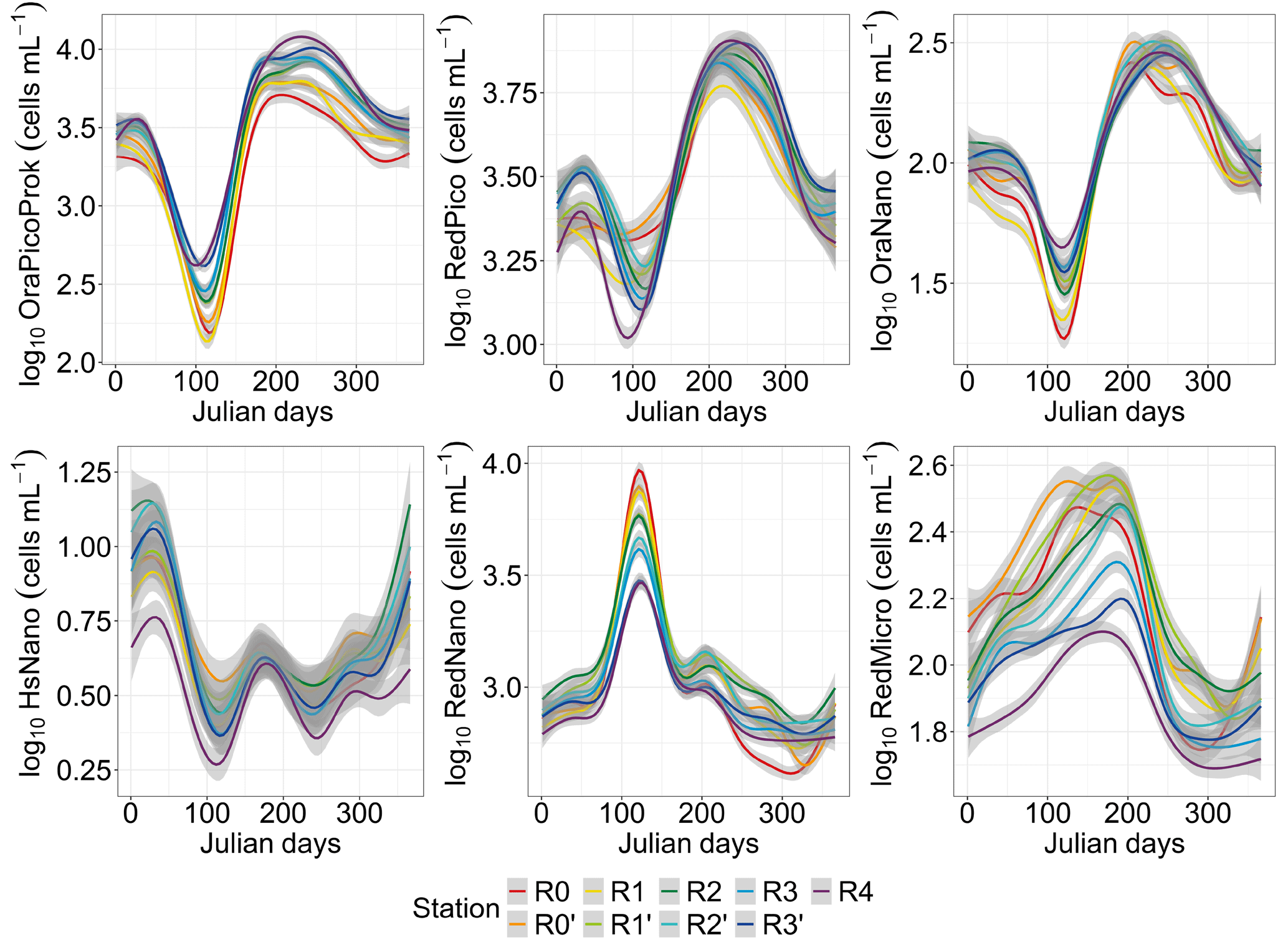
Figure 5 Seasonal and spatial variability in phytoplankton functional group abundance (N=1522 and N interpolated = 35 712). The smoothed curves are modeled per Julian day using a GAM. The shaded area is the confidence interval.

3.2 Spatial and temporal interaction in the Strait of Dover dynamics

For the last decade, the season parameter significantly explained 45 % and 39 % of the variance in the respective environmental variables and phytoplankton communities (PERMANOVA p value <0.05), with a strong difference according to the F statistic score (Tables 1 and 2). The sampling year parameter was the second-most important factor in explaining the variance and influence on phytoplankton abundance (15 %) and on environmental variables (11 %). Finally, over the whole decade, the stations' location along the transect (expressed in longitude) only explained 5 % (very little) of the variance for phytoplankton abundance and environmental variables. The combined factors of year and season explained 6.9 % of the variance for phytoplankton abundance groups and 9.8 % of the variance for abiotic parameters. Pairwise post hoc tests showed that all seasons differed significantly (p value < 0.05) from one another in terms of abiotic parameters, with the exception of autumn and winter for phytoplankton communities (Appendix B1). No significant differences were observed between stations regarding phytoplankton communities with the exception of R0, which was significantly different from all stations with respect to environmental parameters according to Tukey's post hoc test (p value <0.05). Considering the interannual variability, 2020 differed significantly from all other years (except for 2015) with respect to abiotic parameters, while it differed from 2012 and 2017 with respect to phytoplankton communities. In addition, abiotic parameters for 2015 and 2022 also differed from other years in the series (from 2012, 2013, 2017, 2021, 2022 and 2014 for 2015 and from 2015, 2019 and 2020 for 2022). Phytoplankton communities were particularly different from 2017 onwards, with 2020 and 2021 being the most different from all other years.

Table 1 PERMANOVA partitioning and analysis of environmental variables (SST, salinity, [${\mathrm{NO}}_{\mathrm{2}}^{-}$ + ${\mathrm{NO}}_{\mathrm{3}}^{-}$], dissolved P and dissolved Si) from the decadal data, based on range-transformed values and Bray–Curtis dissimilarities. “df” stands for degrees of freedom, the coefficient of determination (R²) explains the variability in the dependent variable and the F statistic evaluates the size effect (the higher the F value, the greater the variation). Bold text indicates a significant effect on variability (p value <0.05).

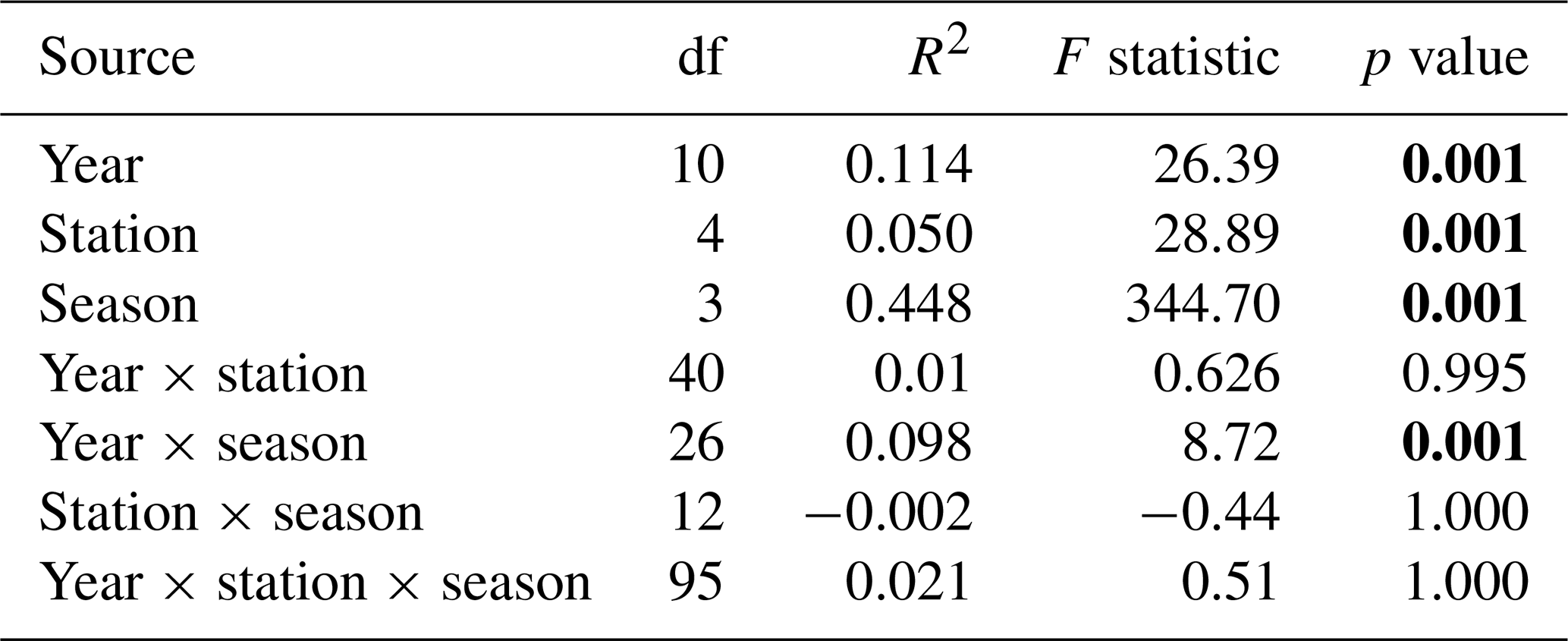
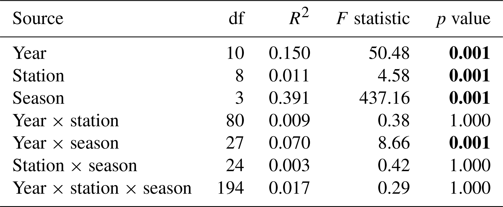
Table 2 PERMANOVA partitioning and analysis of phytoplankton abundance from the decadal data, based on Hellinger-transformed abundances and Bray–Curtis dissimilarities. “df” stands for degrees of freedom, the coefficient of determination (R²) explains the variability in the dependent variable and the F statistic evaluates the size effect (the higher the F value, the greater the variation). Bold text indicates a significant effect on variability (p value <0.05).

3.3 Long-term variability

3.3.1 Environmental decadal evolution

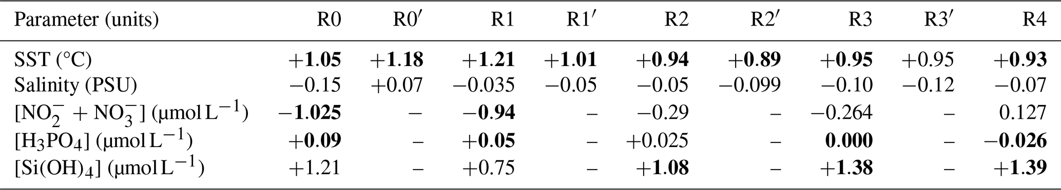
Between 2012 and 2022, the sea surface waters within the nearshore–offshore transect exhibited notable fluctuations in SST, salinity and the concentration of key nutrients (such as nitrite, nitrate, dissolved P and dissolved Si). These variations were analyzed as part of a global approach incorporating both cumulative sums and general trends for each parameter over time. At the beginning of the time series, the cumulative sum analysis for SST (Fig. 6a) indicated below-average values (negative slope) influenced by the starting value. Since 2014, an overall trend toward an SST increase was observed, with a consistently above-average SST (positive slope). Besides some fluctuations, raw data and decadal SST trend analysis corroborated this observation, revealing an overall increase ranging from +0.89 to +1.21 °C between February 2012 and December 2022 (Sen slope values, p value <0.05). Nearshore waters showed more pronounced warming compared with offshore waters (Table 3). Sea surface salinity (Fig. 6b) began with a phase of decline until winter 2013, increased until winter 2019 and then declined again until the end of the study period. Although trend tests failed to detect any significant trends in salinity values over the period (Table 3), all values were negative and in line with the fluctuations observed in both the raw data and cumulative sums. Regarding nutrient levels, the [${\mathrm{NO}}_{\mathrm{2}}^{-}$ + ${\mathrm{NO}}_{\mathrm{3}}^{-}$] concentrations (Fig. 6c) displayed a U-shaped pattern throughout the decadal period, decreasing from particularly high values during winter 2013–2014 ([${\mathrm{NO}}_{\mathrm{2}}^{-}$ + ${\mathrm{NO}}_{\mathrm{3}}^{-}$] > 20 µmol L⁻¹) and then increasing to high values in January 2018 and in winter 2021–2022 ([${\mathrm{NO}}_{\mathrm{2}}^{-}$ + ${\mathrm{NO}}_{\mathrm{3}}^{-}$] > 10 µmol L⁻¹). However, a significant decrease (Mann–Kendall trend analysis) in [${\mathrm{NO}}_{\mathrm{2}}^{-}$ + ${\mathrm{NO}}_{\mathrm{3}}^{-}$] was observed at stations R0 and R1 (nearshore waters) over the whole period (Table 3). The cumulative sum analysis of phosphate concentrations revealed a more intricate pattern (Fig. 6d), characterized by alternating phases of increase and decrease, punctuated by peaks in winter in 2015–2016 and 2019–2020. Trend analysis indicated an overall increase in the phosphate concentration at nearshore stations (R0 and R1; Table 3). Cumulative sums of the dissolved Si concentration depicted a declining trend since winter 2013–2014 except during winter 2019–2020 (Fig. 6e). Raw data highlight elevated concentrations during the winter of 2019–2020. Significant increases in the dissolved Si levels were detected from station R2 (frontal waters) to station R4 (offshore waters) (Table 3). The combined analysis of raw data and cumulative sums enabled us to identify periods of change in physicochemical variables (according to Regier et al., 2019), such as the transition between 2013 and 2014 and the change during the period from 2018 to 2020, by observing changes in the slope. On the other hand, trend tests (Mann–Kendall) and slope calculations (Sen slope estimate) facilitated trend identification and quantification.

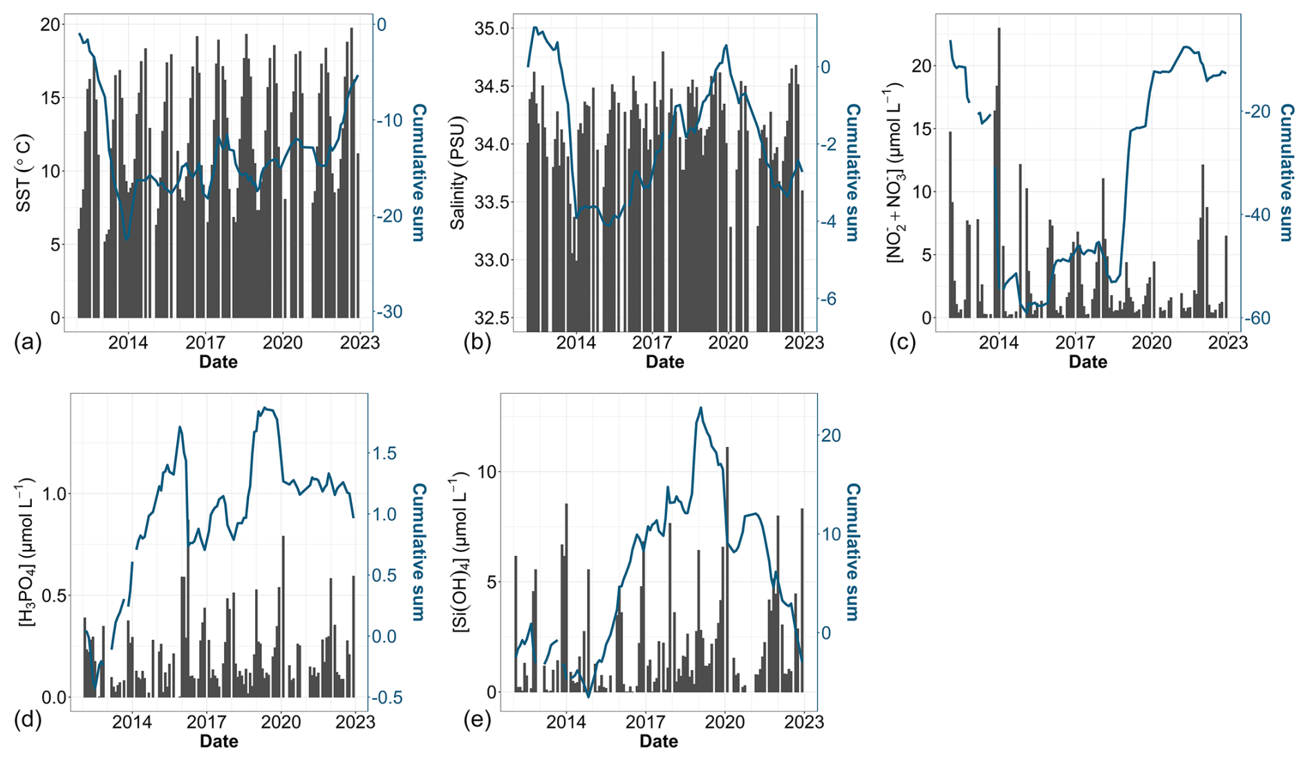
Figure 6 Time series of environmental parameters: (a) SST, (b) salinity, (c) [${\mathrm{NO}}_{\mathrm{2}}^{-}$ + ${\mathrm{NO}}_{\mathrm{3}}^{-}$], (d) [H₃PO₄] and (e) [Si(OH)₄]. Bar plots represent monthly raw data for all stations combined (left y axis). The blue lines correspond to the cumulative sum of anomalies over time (based on the difference between these monthly averages and the monthly average for the period; right y axis).

Table 3 Trends and the magnitude (slope) of change in the SST, salinity, [${\mathrm{NO}}_{\mathrm{2}}^{-}$ + ${\mathrm{NO}}_{\mathrm{3}}^{-}$], dissolved P and dissolved Si from a Mann–Kendall test and Sen slope calculation. Bold text indicates a significant trend (p value <0.05) over the period from 2012 to 2022. The values indicate the magnitude of the trend.

Fluctuations in nutrient concentration have implications with respect to the nutrient ratios and, in turn, underline potential nutrient limitation. Consequently, phytoplankton would respond to these variations through changes in their community composition, biomass and productivity. An assessment of interannual averages across all stations was conducted to investigate annual potential nutrient limitations (Fig. 7). From 2012 to 2015, the system exhibited indications of potential dissolved P limitation (Fig. 7, top part), corresponding to the elevated [${\mathrm{NO}}_{\mathrm{2}}^{-}$ + ${\mathrm{NO}}_{\mathrm{3}}^{-}$] values observed at the beginning of our time series (Fig. 6c). In 2016 and 2017, the nutrient ratios shifted towards a potential dissolved-Si-limited system (Fig. 7, bottom left). Since 2019, a trend towards potential [${\mathrm{NO}}_{\mathrm{2}}^{-}$ + ${\mathrm{NO}}_{\mathrm{3}}^{-}$] limitation has become apparent. However, since 2020, the system seems to be moving towards an equilibrium with respect to the $\mathrm{N}:\mathrm{P}:\mathrm{Si}$ ratio. These shift periods aligned with the break points identified previously with the cumulative sums of [${\mathrm{NO}}_{\mathrm{2}}^{-}$ + ${\mathrm{NO}}_{\mathrm{3}}^{-}$], dissolved P and dissolved Si (Fig. 6c, d and e, respectively). The analysis of these ratios across different seasons (see Appendix A1) reveals that, throughout our time series, winter has moved from a potential dissolved-P-limited situation towards a slightly dissolved-N-limited system. Additionally, the year 2014 exhibits indications of potential dissolved P limitation across all seasons. Furthermore, autumn 2012 and, to a lesser extent, spring 2013 and summer 2018 demonstrate signs of potential dissolved P limitation as well.

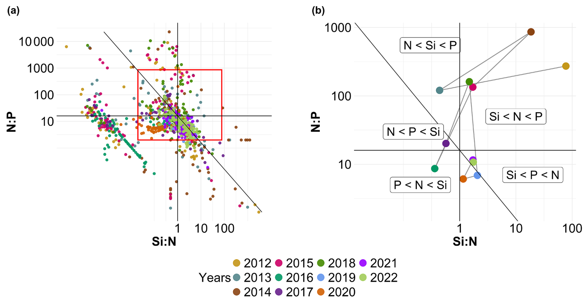
Figure 7 Evolution over time of potential $\mathrm{N}:\mathrm{P}:\mathrm{Si}$ nutrient limitations according to the nutrient ratios ($\mathrm{C}:\mathrm{N}:\mathrm{Si}:\mathrm{P}$ = $\mathrm{106}:\mathrm{16}:\mathrm{16}:\mathrm{1}$; Redfield et al., 1963; Brzezinski, 1985). The horizontal black line represents the N:P limit of 16:1, the vertical black line is the Si:N ratio of 1:1 and the diagonal black line is the Si:P ratio of 16:1. The red box in panel (a) corresponds to the zoomed-in area in panel (b). The large colored dots in panel (b) correspond to the average ratio for each year (N=11), while the small lighter dots in panel (a) correspond to the original raw data of each year (N=1015). The expression A<B means that B is potentially more limiting than A.

3.3.2 Phytoplankton interannual dynamics

Environmental changes observed during the decadal survey have directly affected the biomass, abundance and composition of phytoplankton communities. The integrated analysis, combining total chlorophyll a, as a proxy for phytoplankton biomass, and total abundance revealed distinct patterns (Fig. 8). Chlorophyll a showed a succession of increasing and decreasing phases (Fig. 8a). The initial increase in biomass was notably influenced by the peak of 10.70 µg L⁻¹ in February 2013. During the same year, phytoplankton abundance was remarkably low (Fig. 8b). After this phase, the chlorophyll-a time series showed a decline, notably due to a weak spring bloom in 2016, before moving towards higher values in 2018 and 2021. Despite these fluctuations, statistical tests on the chlorophyll-a concentration revealed no significant decadal trend (Table 4). Conversely, while total cell abundance showed interannual fluctuations, with maximum values over 4×10⁶ cells mL⁻¹ in 2019 and 2021, the analysis of raw data, cumulative sums and the Mann–Kendall test indicated a significant increase over the last decade (Fig. 8b and Table 4).

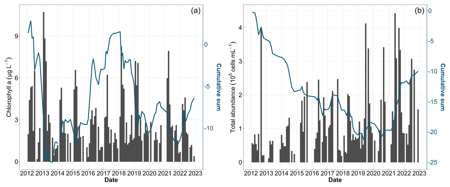
Figure 8 Time series of total phytoplankton biomass using (a) chlorophyll a and (b) total phytoplankton abundance. Bar plots represent monthly raw data for all stations combined (left y axis). The blue lines represent the cumulative sum of anomalies over time (based on the difference between these monthly averages and the monthly average for the period; right y axis).

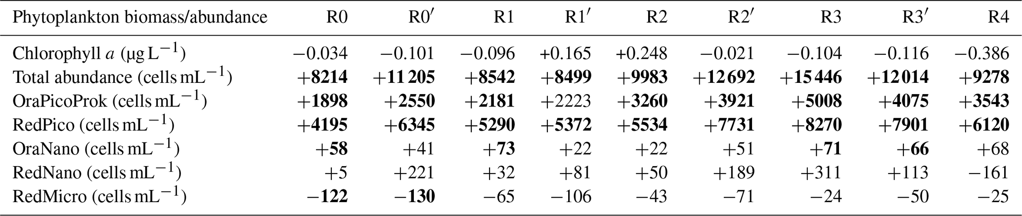
Over the past decade, notable changes in the structure of phytoplankton communities have been observed. Examination of raw data (Fig. 9, black bars) reveals pronounced seasonality, characterized by alternating periods of high and low abundance across all groups. This seasonality, broken down by group, is further presented in Fig. 5. Cumulative sums of various phytoplankton groups indicate a decadal increase in the abundance of OraPicoProk, RedPico and OraNano over the period of our study (Fig. 9a, b and c, respectively). In 2021, OraPicoProk and RedPico exhibited their highest abundance. Furthermore, the high abundance recorded since 2019 for RedPico significantly influenced the trends in these groups as well as the total phytoplankton abundance. Statistical trend analysis confirmed a significant decadal increase in abundance (as well as total abundance) for the latter two groups for all stations (Table 4). OraNano depicted a clear trend for some nearshore and offshore stations as well, whereas a nonsignificant increase characterized frontal and offshore waters. The cumulative sum for RedNano depicts successive phases of increase until 2016, notably attributed to a robust bloom in 2015, followed by a decline until the series' conclusion (Fig. 9d). In spite of a more or less important decadal increase estimated at all stations, no significant trends were evidenced for RedNano. Conversely, RedMicro showed an overall decreasing trend, which has been particularly evident since 2016, and a significant trend was further confirmed at the most coastal stations (Fig. 9e, Table 4).

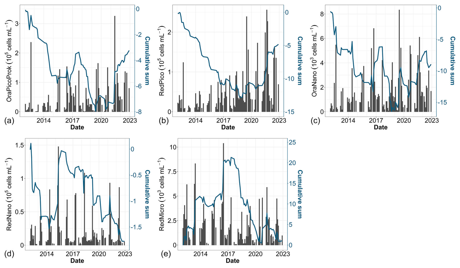
Figure 9 Time series of (a) total abundance, (b) OraPicoProk, (c) RedPico, (d) OraNano, (e) RedNano and (f) RedMicro. Bar plots represent monthly raw data for all stations combined (left y axis). The blue lines represent the cumulative sum of anomalies over time (based on the difference between these monthly averages and the monthly average for the period; right y axis).

Table 4 Trends and the magnitude (slope) of change in phytoplankton chlorophyll a and total and functional group abundance (cells mL⁻¹) determined by flow cytometry from a Mann–Kendall test and Sen slope calculation. Bold text indicates that the trend was significant (p value <0.05) over the period from 2012 to 2022.

4 Discussion

4.1 Decadal trends in physical and chemical parameters

Between 2012 and 2022, the DYPHYRAD time series showed a significant decadal increase in the SST range of between +0.93 and +1.05 °C. This increase was in line with other studies carried out on a larger temporal and/or spatial scales in the English Channel, which reported values of between +0.3 °C per decade to over +1 °C in 5 years (Saulquin and Gohin, 2010; McLean et al., 2019; Cornes et al., 2023). This general increase in SST is linked to an increase in the frequency of the occurrence of maxima. Tinker et al. (2020) highlighted specific years, such as 2014, 2015 and 2017, as amongst the hottest on record with respect to SST over the past 125 years in the EEC region. Data for the year 2022 were not included in these earlier analyses, yet Simon et al. (2023) highlighted a pronounced marine heat wave in 2022, closely associated with exceptionally high air temperatures recorded during that summer (Guinaldo et al., 2023). This phenomenon was also recorded in our time series, which could further corroborate the trend towards increasing SST. This trend is likely to be consolidated in the coming years, as 2023 ranked as the second-hottest year since 1991 (Météo-France). It is noteworthy that the influence of the Atlantic Multidecadal Oscillation (AMO), elucidated by Kerr (2000), has been acknowledged for SST variations in the English Channel (Edwards et al., 2013; Auber et al., 2017). Even though light is a key factor in phytoplankton photosynthesis and the development of phytoplankton communities (Jouenne et al., 2007), it was not taken into account in this study. Moreover, it was not considered in this work because its variability was too dependent on the time of sampling to provide a robust time series, and technical issues led to gaps in the data that were too large for reliable analysis. Regarding salinity, our study did not find any significant trends, even though the study of cumulative sums revealed a period of increasing salinity extending from winter 2014 to winter 2019, followed by a slight decrease during the last years. Salinity is a relatively stable physicochemical parameter, but even the slightest change can have significant implications for the marine environment. Station BL1 ($\mathrm{50}\mathrm{°}{\mathrm{43}}^{\prime }{\mathrm{90}}^{\prime \prime }$ N, $\mathrm{1}\mathrm{°}{\mathrm{33}}^{\prime }{\mathrm{00}}^{\prime \prime }$ E), located around 5.6 km south of our study area, has shown an increase in salinity since 1992 (Lefebvre and Devreker, 2023; Hernández-Fariñas et al., 2014). Increasing sea surface salinity can be attributed to the combined effects of rising SST and a significant reduction in river flows between 1998 and 2019, particularly of the Seine and Somme rivers (Huguet et al., 2024). In our study of the Strait of Dover, the Somme, followed by the Canche, Authie, Liane, Wimereux and Slack, are the rivers that will most influence our sampling area due to increasingly low flow rates. The decrease in river flow over time may be due to a general decrease in rainfall distribution over the last decade (Météo-France, 2025). However, over the past decade, maximum values have tended to increase, which could lead to greater runoff and, therefore, higher concentrations of dissolved phosphorus and silicon due to intense rainfall events. Indeed, dissolved silicon dynamics are linked to the weathering of rocks, 80 % of which are introduced into the ocean by rivers (Conley, 2002). Over the past decade, increasing dissolved Si levels have been noted in frontal and offshore waters (from +1.08 to +1.39 µmol L⁻¹), and an increase in dissolved P has been seen in nearshore waters (from +0.05 to +0.09 µmol L⁻¹), although these values decreased offshore (−0.026 µmol L⁻¹). A previous study at the regional nutrient monitoring (SRN) station BL1 (off the port of Boulogne-sur-Mer) also showed a significant increase in dissolved Si concentrations between 1992 and 2021 but a decrease in dissolved P (Lefebvre and Devreker, 2023). Our study showed a decrease in [${\mathrm{NO}}_{\mathrm{2}}^{-}$ + ${\mathrm{NO}}_{\mathrm{3}}^{-}$] in nearshore waters, thereby confirming the consistent decrease in [${\mathrm{NO}}_{\mathrm{2}}^{-}$ + ${\mathrm{NO}}_{\mathrm{3}}^{-}$] over the 2-decade period (2000–2020; Lheureux et al., 2023). The dominant forms of dissolved nitrogen in the EEC are nitrite and nitrate, and these species are strongly influenced by continental inputs as well as Atlantic offshore inputs and atmospheric deposition (Dulière et al., 2019). The greater reduction in dissolved nitrogen in nearshore compared with offshore waters could be explained by a reduction in continental inputs due to lower river flows along the French coast (Huguet et al., 2024), combined with the implementation of European directives (the Water Framework Directive, WFD, and the MSFD), the latter of which are aimed at reducing inputs of nitrogen and phosphorus into aquatic systems (Vigiak et al., 2023). Conversely, rising SST may lead to increased phosphate release from sediments, which could explain the rise in dissolved phosphorus concentrations despite attenuation efforts (Wu et al., 2014; Vigiak et al., 2023). Added to these long-term trends are occasional events. Winter 2013–2014 emerged as a remarkable period during which the [${\mathrm{NO}}_{\mathrm{2}}^{-}$ + ${\mathrm{NO}}_{\mathrm{3}}^{-}$] concentration was the highest. This is especially meaningful in the context of the extreme weather events of winter 2013–2014, characterized by strong storm events and unprecedented rainfall, resulting in remarkably high turbidity levels (Matthews et al., 2014; Gohin et al., 2015; Masselink et al., 2016). The high dissolved P concentration was particularly notable in the winters of 2015 and 2019. These changes in temperature and nutrient concentration over the decade can modify stoichiometric ratio values (Redfield et al., 1963; Brzezinski, 1985) and lead to different potential resource limitations in the environment, thereby affecting the composition and dynamics of phytoplankton communities.

4.2 Consequences on phytoplankton functional groups

Rising SSTs, decreasing annual river flows, nitrogen depletion and modification of nutrient stoichiometry can lead to a decline in phytoplankton biomass, primary production and certain phytoplankton communities (such as diatoms), as shown in recent studies in the North Sea and English Channel (Capuzzo et al., 2018; Breton et al., 2022; Holland et al., 2023b). This phenomenon of microphytoplankton abundance decreasing to the benefit of small cells, in particular Synechococcus spp. cyanobacteria, has been described by Schmidt et al. (2020) in the Western English Channel (L4 station, 2007–2018). Despite the natural oscillations, the overall rise in the SST may directly impact the physicochemical characteristics of water masses along the DYPHYRAD transect and affect their resident phytoplankton organisms (Richardson and Schoeman, 2004). Increasing temperature has a significant effect on the cell size of phytoplankton communities and their shift to small species (Zohary et al., 2017; Sommer et al., 2017b; Zohary et al., 2021). Combined with a decrease in nutrient availability, this phenomenon is amplified from 4.7 % °C⁻¹ to 46 % °C⁻¹ (Peter and Sommer, 2013). El Hourany et al. (2021) showed the same behavior of phytoplankton communities (constant chlorophyll-a concentration, decrease in diatom abundance and increase in cyanobacteria abundance) in the Mediterranean when faced with a 0.4°C per decade increase in the mean surface temperature. Analysis of these annual limitations over time (Fig. 7) has shown that the ecosystem is not limited by nitrogen, unlike temperate coastal regions where nitrogen generally limits primary production (Blomqvist et al., 2004). Indeed, Lefebvre et al. (2011) described dissolved Si and P as the main limiting nutrients in the EEC. This limitation varies greatly with season and has consequences for the succession of the phytoplankton communities. Notably, diatoms, a key phytoplankton group, have shown a strong positive association with dissolved Si availability and dissolved inorganic nitrogen (DIN; Leynaert et al., 2002; Hernández-Fariñas et al., 2014). Over the past decade, we observed similar trends in nutrient ratios to those observed for the SOMLIT (South of Boulogne-sur-Mer, National Observation Service of the Research Infrastructure ILICO) coastal station, with a decrease in the N:P, Si:P and Si:N ratios (Lheureux et al., 2023). Under these nutrient conditions, small cells become more competitive due to lower resource requirements and a higher surface : volume ratio (Sommer et al., 2017a). However, they are less nutritious primary producers of higher-food-web organisms, which can lead to a decline in higher trophic levels (Schmidt et al., 2020; Holland et al., 2023b). Sommer et al. (2017b) also predict that, with a smaller phytoplankton community, a greater proportion of primary production will benefit the microbial food web, to the detriment of the classic grazing food chain.

4.3 Phytoplankton variability dominated by seasonality

Our study showed that season explained more than 50 % of the variability observed in phytoplankton communities. This seasonality has been described in numerous studies, notably in regards to the spring bloom of Phaeocystis globosa, which can account for up to 80 % of the total phytoplankton biomass in the EEC (Bonato et al., 2016; Guiselin, 2010). The rest of the time, phytoplankton biomass determined by microscope observation (thus excluding picophytoplankton and small nanophytoplankton) is mainly dominated by diatoms and can reach 85 % of total phytoplankton biomass (Breton et al., 2000; Lefebvre et al., 2011; Hernández-Fariñas et al., 2014). In terms of abundance, cyanobacteria, picoeukaryotes and Phaeocystis globosa dominate the area (Bonato et al., 2016). Winter and summer periods are dominated, in terms of abundance, by Synechococcus spp. and picoeukaryotes (Bonato et al., 2016); these species may not share the same niches/habitats (Louchart et al., 2024), allowing them to bloom at the same period (Fig. 5). Other groups are also present in lower abundances, such as cryptophytes, coccolithophores and dinoflagellates (Hernández-Fariñas et al., 2014; Bonato et al., 2016). A spatial gradient is present for most groups, and it is strongly marked for nano- and microphytoplankton, with abundances sometimes 3 times higher at the coast, especially during bloom periods, because there are more resources available nearshore (due to riverine inputs). During the autumn–winter period, changes in the spatial community structure were observed, with the lower abundance of dominant chlorophyll-a nanophytoplankton at nearshore (R0) and offshore (R4) stations compared with frontal stations (R1^′ and R2). This spatial conformation can be explained by the action of coastal flow on water bodies, as well as by the action of tides, wind speed and wind direction (Brylinski et al., 1991; Sentchev and Yaremchuk, 2007). This accumulation of nanophytoplankton in the frontal zones has already been shown (in the southern North Sea) to be linked to the greater presence of nutrients in these structures than in other bodies of water (Gieskes et al., 2007). Our study has also highlighted the importance of bottom-up control on phytoplankton abundance and biomass distribution, but other parameters, such as zooplankton predation (Cotonnec et al., 2001; Breton et al., 2021) and seasonal bacterial/microbial and viral interactions, can play a significant role in phytoplankton community variability (Brussaard, 2004; Lamy et al., 2009).

4.4 General discussion, limitations and perspectives

The sampling strategy within DYPHYRAD surveys allowed for the acquisition of additional phytoplankton-related data at higher sampling frequencies and finer spatial scales than other such monitoring networks (SOMLIT, SRN-REPHY and PHYTOBS). Although our approach is also characterized by a fine spatial resolution, its temporal resolution is lower than the high-frequency moorings or automated stations of the French national Coast-HF network (the MAREL Carnot automated station off Boulogne-sur-Mer; Halawi Ghosn et al., 2023). Moreover, our surveys made it possible to decouple stations in order to account for the entire coast–offshore gradient – a frontal zone separating waters influenced by desalination from river inputs and offshore waters under a macrotidal regime, thereby considering tidal variability. Most long-term studies on the evolution of phytoplankton communities over time are either based on the evolution of chlorophyll a, as a proxy for phytoplankton biomass to explain changes linked to environmental parameters, or on taxonomical phytoplankton counts by microscopy. However, this kind of approach does not seem sufficient, as it neglects the influence of smaller groups (e.g., picoeukaryotes, cyanobacteria and small nanophytoplankton; McQuatters-Gollop et al., 2024) that play an essential role in food webs. The advantage of automated pulse-shape flow cytometry is that the methodology is the same for the analysis of the entire phytoplankton size range (Dubelaar et al., 2004), in vivo, avoiding any damage or effect of fixatives. The optical characteristics of each particle can then be used to monitor not only abundance but also functional traits specific to each phytoplankton functional group (Fontana et al., 2018; Fragoso et al., 2019; Louchart et al., 2020). Although this method enables us to study all phytoplankton, it is not a taxonomic technique (except in the case of microphytoplankton via CytoSense photo acquisition) and could be combined with approaches enabling finer identification. In order to exploit these features and upscale such results over the long term, it remains essential to improve standard operating procedures for better intercomparability and interoperability between machines; such work is still in progress in the framework of current international projects such as JERICO-S3 and OBAMA-NEXT.

5 Conclusions

This local-scale study showed an increase in SST, nearshore dissolved P and offshore dissolved Si as well as a decrease in the [${\mathrm{NO}}_{\mathrm{2}}^{-}$ + ${\mathrm{NO}}_{\mathrm{3}}^{-}$] concentration in nearshore water over the last decade. Pulse-shape flow cytometry time series allowed for the exploration of the spatiotemporal in vivo dynamics of almost the whole phytoplankton community. A significant increase in small phytoplankton (including cyanobacteria) and a decrease in microphytoplankton abundance (in coastal water) were evidenced. While our time series is too short to draw definitive conclusions about long-term and complex climate change impacts, it allows us to make an initial assessment of change within phytoplankton communities in the EEC by the Strait of Dover. Recent studies have increasingly indicated that climate change is a driver of major alterations in oceanic and coastal ecosystems, particularly through increases in the SST and nutrient availability (Pörtner et al., 2022). Such environmental transformations influence the phytoplankton community size by favoring smaller phytoplankton species and cyanobacteria, which are more adaptable to warmer and nutrient-variable conditions (Sommer et al., 2017b; Zohary et al., 2017, 2021). The reduction in microphytoplankton observed here could signify a broader shift toward smaller phytoplankton sizes in response to these pressures, impacting trophic dynamics by influencing size-grazing, nutrient consumption and sedimentation as well as limiting the energy transfer efficiency within the food web. As climate models predict continued warming and nutrient shifts (Pörtner et al., 2022), these initial changes observed in the Strait of Dover may signal a broader trend, making sustained monitoring and high-resolution data critical to anticipate long-term impacts on marine biodiversity and ecosystem stability. It is crucial to sustain sampling efforts using automated techniques like flow cytometry to exhaustively monitor the evolution of phytoplankton dynamics. This monitoring should be integrated as a complement of existing low-frequency reference national and regional observation networks and incorporated into high-frequency survey efforts, as carried out in previous short-term studies on automated stations (Thyssen et al., 2014; Robache et al., 2025), ships of opportunity (Marrec et al., 2021) and oceanographic cruises (Bonato et al., 2016; Louchart et al., 2020, 2024). Supported by a more comprehensive characterization of PFGs, this approach will greatly enhance our understanding of the impacts of global and anthropogenic changes on phytoplankton functional diversity. Moreover, when coupled with productivity measurements (Aardema et al., 2019) and integrated into predictive models, it becomes possible to evaluate the potentialities of food web evolution and overall ecosystem function.

Appendix A: Seasonal nutrient limitation

To study the evolution of nutrient limitation in more detail within the annual evolution, we analyzed seasonal $\mathrm{N}:\mathrm{P}:\mathrm{Si}$ (dissolved nitrogen : dissolved phosphorus : dissolved silicon) ratios (Fig. A1). This representation shows near constancy in winter seasons with little or no potential dissolved Si limitation and only slight dissolved P or dissolved N limitation. Spring shows a potential dissolved P limitation for the years 2013, 2014, 2015 and 2018, whereas the other years do not seem to be limited or are only slightly limited by dissolved Si or dissolved N. Autumn 2015 and 2020 appear to be potentially limited by dissolved Si, whereas 2012 and 2014 show a clear dissolved P limitation. Summer 2014 and 2018 tend to be slightly potentially limited by dissolved P, while summer 2013, 2015 and 2016 tend to be potentially limited by dissolved Si. The other summer seasons do not appear to be limited or are only slightly potentially limited by dissolved N, according to the data presented here.

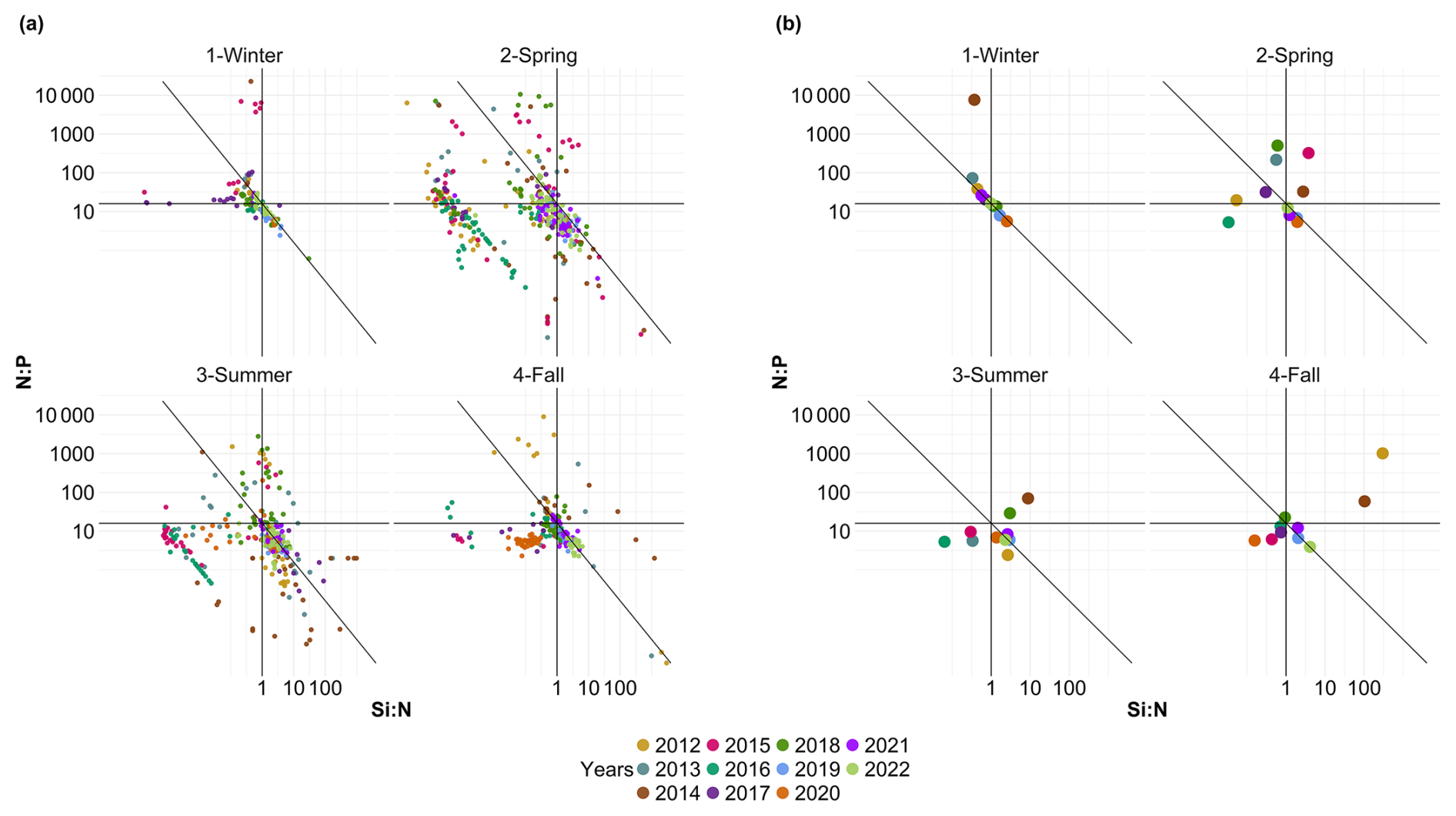
Figure A1 Evolution of potential $\mathrm{N}:\mathrm{P}:\mathrm{Si}$ nutrient limitations over the seasons according to the nutrient ratios ($\mathrm{C}:\mathrm{N}:\mathrm{Si}:\mathrm{P}$ = $\mathrm{106}:\mathrm{16}:\mathrm{16}:\mathrm{1}$; Redfield et al., 1963; Brzezinski, 1985). The horizontal line represents the N:P limit of 16:1, the vertical line is the Si:N ratio of 1:1 and the diagonal line is the Si:P ratio of 16:1. Small dots in panel (a) correspond to original raw data of each year (N=1015), whereas the colored dots in panel (b) correspond to the average ratio for each year and season (N=44).

Appendix B: The Tukey post hoc test results

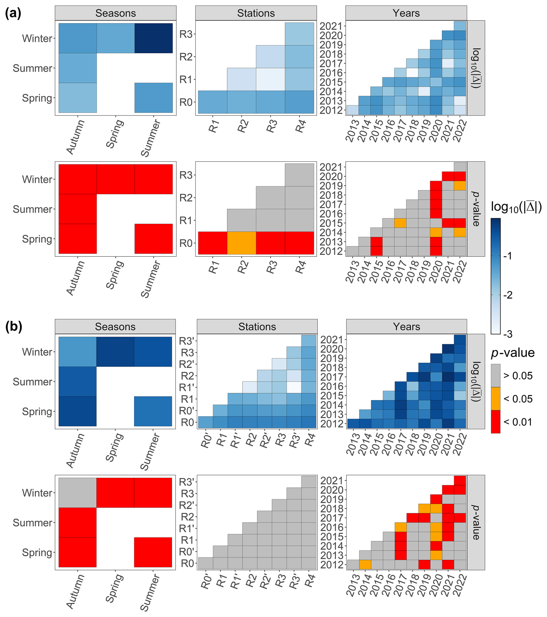
Figure B1 The Tukey post hoc results for (a) environmental data and (b) phytoplankton abundance data. The absolute value of the mean difference provided by the test (noted $\left|\stackrel{\mathrm{‾}}{\mathrm{\Delta }}\right|)$ and the associated p value are provided.