Turbulent heat flux dynamics along the Dotson and Getz ice-shelf fronts (Amundsen Sea, Antarctica)

In coastal polynyas, where sea-ice formation and melting occur, it is crucial to have accurate estimates of heat fluxes in order to predict future sea-ice dynamics. The Amundsen Sea Polynya is a coastal polynya in Antarctica that remains poorly observed by in situ observations because of its remoteness. Consequently, we rely on models and reanalysis that are un-validated against observations to study the effect of atmospheric forcing on polynya dynamics. We use austral summer 2022 shipboard data to understand the turbulent heat flux dynamics in the Amundsen Sea Polynya and evaluate our ability to represent these dynamics in ERA5. We show that cold- and dry-air outbreaks from Antarctica enhance air–sea temperature and humidity gradients, triggering episodic heat loss events. The ocean heat loss is larger along the ice-shelf front, and it is also where the ERA5 turbulent heat flux exhibits the largest biases, underestimating the flux by up to 141 W m⁻² due to its coarse resolution. By reconstructing a turbulent heat flux product from ERA5 variables using a nearest-neighbor approach to obtain sea surface temperature, we decrease the bias to 107 W m⁻². Using a 1D model, we show that the mean co-located ERA5 heat loss underestimation of 28 W m⁻² led to an overestimation of the summer evolution of sea surface temperature (heat content) by +0.76 °C (+8.2×10⁷ J) over 35 d. By obtaining the reconstructed flux, the reduced heat loss bias (12 W m⁻²) reduced the seasonal bias in sea surface temperature (heat content) to −0.17 °C (−3.30 × 10⁷ J) over the 35 d. This study shows that caution should be applied when retrieving ERA5 turbulent flux along the ice shelves and that a reconstructed flux using ERA5 variables shows better accuracy.

1 Introduction

Among other properties such as momentum, gas, and moisture, the atmosphere and the ocean exchange heat, which maintains the Earth's energy balance (Yu, 2019). The climate is highly controlled by the ocean, notably because the ocean has the ability to absorb heat from the atmosphere and to redistribute it poleward (Bigg et al., 2003). The ocean is thus the largest heat sink on Earth, absorbing 91 % of the excess heat due to greenhouse gases (Forster et al., 2021). The exchange of heat between the ocean and the atmosphere – or air–sea heat flux – is therefore a crucial process to predict the current and future weather (through heat and moisture released into the atmosphere), upper-ocean physics (sea surface temperature (SST) variability, sea-ice formation and melting, heat content (HC) in the mixed layer), climate (e.g., teleconnections such as El Niño), and the ensuing impacts on society (e.g., agriculture, health, water resources) (Cronin et al., 2019). Because of the importance of air–sea heat fluxes, the scientific community calls for reducing uncertainties to have better flux estimates (Cronin et al., 2019). By increasing the number of observations, our understanding of fluxes can be enhanced and the associated uncertainties reduced (Cronin et al., 2019; Swart et al., 2019; Yu, 2019; Bourassa et al., 2013).

Polar regions are poorly observed because of their remoteness and harsh conditions, which implies that we have a particular lack of understanding of the flux dynamics there. In particular, the Southern Ocean south of 60° S has been identified by Swart et al. (2019) as a targeted observation region for the ongoing decade. The Amundsen Sea, West Antarctica (Fig. 1), is a shelf sea south of 60° S seasonally covered by sea ice and with few historical observations. However, scientific efforts have been concentrated there recently, for example, through the International Thwaites Glacier Collaboration (Turner et al., 2017; Scambos et al., 2017) due to adjacent melting glaciers and one of the most biologically productive coastal polynyas (the Amundsen Sea Polynya, ASP) in the Antarctic (Arrigo and van Dijken, 2003).

Polynyas are defined based on their opening mechanism. The ASP is a wind-driven latent heat polynya that forms along the coastline. It has a mean open-water area in the austral summer of 27 333 km²± 8749 km² and an average duration of 131.9 ± 17.5 d over 1997–2010 (Arrigo et al., 2012). In comparison to the surrounding sea ice that acts as a lid, the polynya operates as an open window that enables direct exchange with the atmosphere (Smith and Barber, 2007). During winter, shelf water latent heat polynyas like the ASP usually gain the “sea-ice factory” nickname (Morales Maqueda et al., 2004; Ohshima et al., 1998) because sea ice is continually created and conveyed away by winds or currents. On the other hand, in summer the latent heat polynyas are “ice-melting factories”, as the low albedo of open water compared to the surrounding sea ice favors solar heating, resulting in melting sea ice. To be able to better predict sea-ice formation and melting in the Amundsen Sea, we therefore need to improve our knowledge of heat exchange in the ASP region.

Air–sea heat fluxes must also be considered in the context of the broader atmospheric circulation. In the Southern Ocean near the polar front at 54° S, 89° W, Ogle et al. (2018) show that the advection of cold and dry air triggers ocean heat loss. In the Amundsen Sea, Papritz et al. (2015) showed from ERA-Interim data that the Amundsen Sea is a hotspot for cold-air outbreaks (CAOs), which contribute to the turbulent loss. CAOs are the equatorward intrusion of cold air over the warmer ocean (Papritz et al., 2015). The large-scale atmospheric system also impacts sea ice: in 2022, the Amundsen Sea Low (ASL), a quasistationary low-pressure center, enhanced sea-ice melting (Turner et al., 2022; Yadav et al., 2022).

Without available air–sea heat flux observations, previous studies in the Amundsen Sea or other Antarctic coastal seas have relied on global reanalysis products (e.g., Kumar et al., 2021; Zhou et al., 2022; Yu et al., 2023; Papritz et al., 2015). A global climate reanalysis product combines observations and past forecasts through data assimilation, providing gridded data with a regular temporal resolution. The ERA5 reanalysis, produced by the European Centre for Medium-range Weather Forecasts (ECMWF;  Hersbach et al., 2020) and its predecessor (ERA-Interim) are considered the most robust reanalyses in Antarctica (Bromwich et al., 2011; Bracegirdle and Marshall, 2012) and in the Amundsen Sea (Jones et al., 2016; Jones, 2018). However, ERA5's ability to reproduce the flux magnitude and variability in the Amundsen Sea, particularly near important boundaries such as ice-shelf fronts, has not been validated.

The air–sea heat flux has two components: the radiative flux (sum of the shortwave and longwave radiation) and the turbulent flux (sum of the sensible and latent fluxes). The turbulent heat flux is the main air–sea heat flux component during winter, whereas the radiative component dominates during summer (Morales Maqueda et al., 2004). Despite the importance of the radiative component in summer, key atmospheric conditions could set the scene for important episodic heat loss events. We hypothesize that the Amundsen Sea has high potential for turbulent loss due to cold, dry air and relatively warm SST in summer (above freezing temperature). We perform the first study of the turbulent heat flux (THF) in the Amundsen Sea based on austral summer in situ observations, and we (i) identify the temporal and spatial variability in the 2022 THF from shipboard observations, (ii) assess ERA5's accuracy at representing these fluxes, and (iii) investigate the relative importance of THF on the summer evolution of SST. Our findings provide evidence of the synoptic-scale air–sea interactions in the ASP and their impact on the summer evolution of SST.

2 Data and methods

2.1 Data

2.1.1 Observations – shipboard and glider data

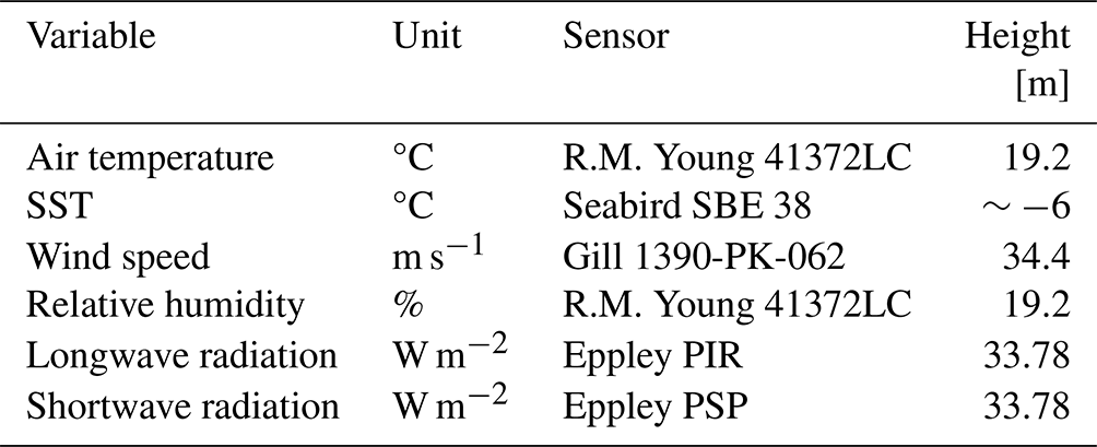
The meteorology system and thermosalinograph of the research vessel (RV) Nathaniel B. Palmer recorded the variables listed in Table 1 over 57 d. We use these observations to compute the bulk THF; the computation method is described in Sec. 2.2.1. The ship departed Punta Arenas (Chile) on 6 January 2022, reaching the Amundsen Sea (72° S, 117° W) on 15 January 2022. It then entered the polynya region and spent 31 d within 20 km of the Dotson or Getz ice shelves and finally left the polynya region on 25 February 2022 (Fig. 1b). To determine the THF and be consistent with ERA5's temporal resolution, we compute hourly means of the variables in Table 1. The initial resolution was 1 min. The hourly position of the ship is used to create a classification: Southern Ocean, open ocean in the polynya region (ship more than 20 km away from the coastline), in front of the Dotson or Getz ice shelves (ship within 20 km), and in a sea-ice-covered region (where the sea-ice concentration (SIC) is larger than 0.15). The RV Nathaniel B. Palmer presumably avoided regions of higher sea-ice concentration on its transit to the Amundsen Sea. Airflow distortion of the wind speed values caused by the superstructure of the RV Nathaniel B. Palmer was negligible (Appendix A, Fig. A1); we therefore did not perform any correction. Several conductivity, temperature, and depth (CTD) casts were taken during the research campaign. In the present study we use one, taken at 74.02° S, 113° W in front of Dotson Ice Shelf (Fig. 1a, blue square) to initialize the 1D PWP (Price–Weller–Pinkel) model (see the model description in Sect. 2.2.2).

Table 1 Sensors installed and variables used in this study recorded by the RV Nathaniel B. Palmer.

We use Conservative Temperature, Absolute Salinity, and pressure from an ocean profiling Seaglider that was deployed during the ship campaign to compute the daily HC in the upper 40 m of the water column. The glider was deployed on 17 January 2022 in front of Dotson Ice Shelf (73.8° S, 112.6° W). It sampled to the seabed, with a maximum of 901 m, surfacing between each dive. The glider then headed south towards the ice shelf and returned north along the Dotson–Getz trough before being recovered on 4 February 2022 (red transect, Fig. 1a). A total of 286 profiles were collected. The data are gridded horizontally per profile and vertically with a resolution of 2 m.

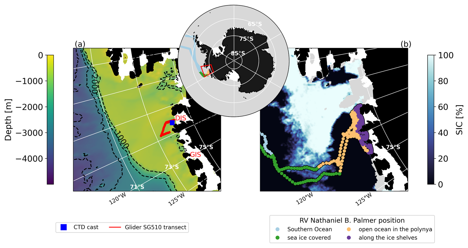
Figure 1 (a, b) Antarctica in black, with ice shelves from BedMachine (Morlighem et al., 2020) in white. (a) The background is bathymetry from RTopo (Schaffer et al., 2016); the blue square is the CTD cast location used to force the 1D model, and the glider transect is in red. Dotson and Getz ice shelves (DIS; GIS) are indicated in red. (b) Sea-ice concentration from the ARTIST sea ice (ASI) algorithm on 19 February 2022 (downloaded from https://data.seaice.uni-bremen.de, last access: 13 January 2025; Spreen et al., 2008); the RV transect is indicated by the points colored by the location classification. The red box on the zoomed-out map is the Amundsen Sea plotted on (a) and (b).

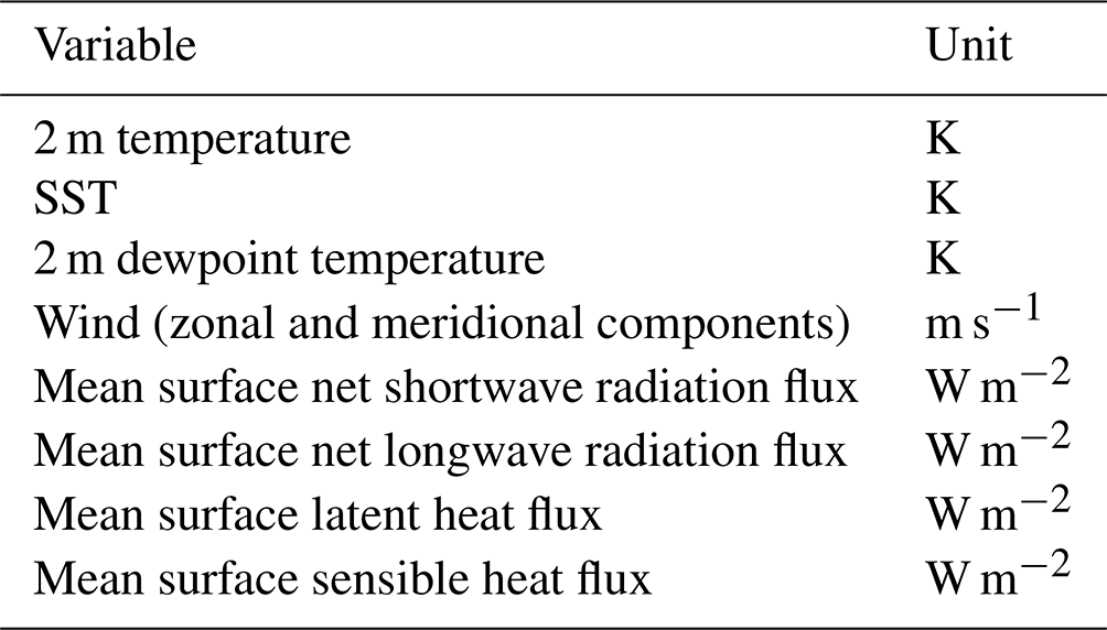
2.1.2 Reanalysis dataset – ERA5

In this study, we assess ERA5 by comparing its hourly mean THF with the THF computed from the observations. We also use some of ERA5's hourly mean meteorological and sea surface variables to recalculate the THF (Table 2). ERA5 is a global reanalysis product that provides “maps without gap” of atmospheric and sea surface variables (Hersbach et al., 2020). It has a hourly temporal resolution and a regular 0.25° latitude–longitude grid. To co-locate its variables to the ship data, we use the nearest-neighbor grid cell and the corresponding hour (as the ship data have been hourly averaged).

Table 2 ERA5 variables used in this study.

2.1.3 Satellite-based data – sea-ice concentration from the ARTIST sea-ice algorithm

We use sea-ice concentration to determine when the research vessel was surrounded by sea ice (15 % threshold) for the location classification (Fig. 1b). We select the satellite-based sea-ice product ARTIST sea ice (ASI) created by Bremen University (Spreen et al., 2008, data downloaded from https://data.seaice.uni-bremen.de/amsr2). The ASI algorithm takes input data from the Advanced Microwave Scanning Radiometer 2 (AMSR2, Level 1B) – a sensor operating on the JAXA satellite GCOM-W1 – and outputs gridded data (Level 3, grid space is 3.125 or 6.25 km). The temporal resolution is daily; the selected output grid space for this study is 3.125 km. The ASI algorithm has been validated against observations and shows good performance (Spreen et al., 2008). It should be noted that during the research cruise, the sea ice gradually melted, so from February 2022 onwards, we can no longer really speak of a polynya, as only a tongue of ice attached to Thwaites Ice Shelf remains visible in the satellite-derived product (https://data.seaice.uni-bremen.de/databrowser/, last access: 13 January 2025). We therefore refer to the polynya region.

2.2 Methods

2.2.1 Turbulent heat flux computation and analyses – COARE 3.5 algorithm, Reynolds decomposition, and indices of contribution

The THF is the sum of the latent heat flux (LHF) and the sensible heat flux (SHF). The LHF is related to the air–sea heat exchange originating from the sea surface evaporation, whereas the SHF arises from the air–sea temperature gradient. We use the Coupled Ocean–Atmosphere Response Experiment (COARE) 3.5 algorithm (Edson et al., 2013) through AirSeaFluxCode (Biri et al., 2023) to compute the THF from the observations. The COARE 3.5 algorithm relies on bulk parameterizations: the LHF and SHF are computed as a function of air density (ρ_air), wind speed measured at height z_u ($U_{z_u}$), the transfer coefficient corresponding to the measured height z_m of humidity and temperature, and the measured height z_u of the wind speed (C_q(z_m,z_u) or C_t(z_m,z_u)). For the SHF (Eq. 1), the specific heat capacity (C_p) and air–sea temperature gradient $(T_{\mathrm{air},z_{\mathrm{m}}}-T_{\mathrm{skin}})$ are calculated; for the LHF (Eq. 2), the latent heat of vaporization (L_v) and air–sea humidity gradient $(q_{\mathrm{air},z_{\mathrm{m}}}-q_{\mathrm{sat}})$ are calculated.

$$\begin{array}{}\text{(1)}& {\displaystyle }\mathrm{SHF}={\mathit{\rho }}_{\mathrm{air}}{C}_{\mathrm{p}}{C}_{\mathrm{t}}(z_{\mathrm{m}},z_u)U_{z_u}(T_{\mathrm{air},z_{\mathrm{m}}}-T_{\mathrm{skin}})\text{(2)}& {\displaystyle }\mathrm{LHF}={\mathit{\rho }}_{\mathrm{air}}{L}_{\mathrm{v}}{C}_q(z_{\mathrm{m}},z_u)U_{z_u}(q_{\mathrm{air},z_{\mathrm{m}}}-q_{sat})\end{array}$$

The AirSeaFluxCode applies a logarithmic correction to the transfer coefficient definitions (C_t(z_m,z_u) and C_q(z_m,z_u)) to account for the height z_u of wind speed and z_m of air temperature and humidity measurements (Biri et al., 2023). Atmospheric stability is accounted for in the definition of the transfer coefficients C_t and C_q through stability functions. The measured relative humidity is converted to saturated humidity using the saturation vapor pressure function from Buck (2012). Warm-layer and cool-skin corrections are applied to convert the measured SST (Table 1) to skin SST, as is required in Eq. (1). These corrections follow Fairall et al. (1996). The COARE 3.5 algorithm requires wind speed relative to the ocean surface. Here, we assume that the ocean currents are low in comparison to the wind speed and neglect them. We find this reasonable, as Kim et al. (2016) have shown from recording current meters installed on a 2-year mooring that the coastal surface current in the Amundsen Sea is about 0.2 cm s⁻¹, which is 0.03 % of the mean wind speed (7.9 m s⁻¹; Fig. 2a) in our dataset. The flux convention is downward, which means that a negative (positive) flux corresponds to a heat loss (gain) for the ocean surface.

To account for the insulating effect of sea ice, we scale the turbulent fluxes by the sea-ice concentration (SIC) when SIC ≥ 15 % (Eqs. 3, 4, and 5). We acknowledge that this is a simplified method to account for the sea-ice effect on turbulent fluxes but accept this, considering the small amount of time spent by the RV in a sea-ice-covered area (3 d out of 57 d) and the low importance of the flux variability in sea ice for the results of this study.

$$\begin{array}{}\text{(3)}& {\displaystyle }\mathrm{LHF}=(\mathrm{1}-\mathrm{A})\mathrm{LHF},\text{(4)}& {\displaystyle }\mathrm{SHF}=(\mathrm{1}-\mathrm{A})\mathrm{SHF},\end{array}$$

where

$$\begin{array}{}\text{(5)}& \mathrm{A}=\left\{\begin{array}{ll}\mathrm{SIC}& \mathrm{if}\mathrm{SIC}\ge \mathrm{0.15}\\ \mathrm{0}& \mathrm{if}\mathrm{SIC}<\mathrm{0.15}\end{array}\right..\end{array}$$

We perform a Reynolds decomposition to analyze the flux variability. We decompose SHF and LHF into the sum of their average (denoted by an overline) and their anomaly (denoted by ^′): SHF = $\stackrel{\mathrm{‾}}{\mathrm{SHF}}$ + SHF^′ and LHF = $\stackrel{\mathrm{‾}}{\mathrm{LHF}}$ + LHF^′. We follow the same method as in Tanimoto et al. (2003), Chuda et al. (2008), and Yang et al. (2016) except that we do not neglect the contributions of $C_q^{\prime }$ and $C_{\mathrm{t}}^{\prime }$, as they are more than 5 % of their mean values (not shown; criteria following Cayan, 1992). We replace the variables $U_{z_u}$, $\mathrm{\Delta }T=T_{\mathrm{air},z_{\mathrm{m}}}-T_{\mathrm{skin}}$, $\mathrm{\Delta }q=q_{\mathrm{air},z_{\mathrm{m}}}-q_{\mathrm{sat}}$, C_q, and C_t in Eqs. (1) and (2) with the sum of their mean and anomaly (details in Appendix B). Finally, we obtain

$$\begin{array}{}\text{(6)}& {\displaystyle }\begin{array}{rl}& {\mathrm{SHF}}^{\prime }=\mathrm{SHF}-\stackrel{\mathrm{‾}}{\mathrm{SHF}}=\\ & {\mathit{\rho }}_{\mathrm{air}}{C}_{\mathrm{p}}[\underset{\text{t term}}{\underbrace{\mathrm{\Delta }{T}^{\prime }\stackrel{\mathrm{‾}}{U}\stackrel{\mathrm{‾}}{C_{\mathrm{t}}}}}+\underset{\text{u term}}{\underbrace{\stackrel{\mathrm{‾}}{\mathrm{\Delta }T}{U}^{\prime }\stackrel{\mathrm{‾}}{C_{\mathrm{t}}}}}+\underset{\text{ct term}}{\underbrace{\stackrel{\mathrm{‾}}{\mathrm{\Delta }T}\stackrel{\mathrm{‾}}{U}{C}_{\mathrm{t}}^{\prime }}}+\underset{\text{t–u term}}{\underbrace{\stackrel{\mathrm{‾}}{C_{\mathrm{t}}}(\mathrm{\Delta }{T}^{\prime }{U}^{\prime }-\stackrel{\mathrm{‾}}{\mathrm{\Delta }{T}^{\prime }{U}^{\prime }})}}\\ & +\underset{\text{t–ct term}}{\underbrace{\stackrel{\mathrm{‾}}{U}(\mathrm{\Delta }{T}^{\prime }{C}_{\mathrm{t}}^{\prime }-\stackrel{\mathrm{‾}}{\mathrm{\Delta }{T}^{\prime }{C}_{\mathrm{t}}^{\prime }})}}+\underset{\text{u–ct term}}{\underbrace{\stackrel{\mathrm{‾}}{\mathrm{\Delta }T}(U^{\prime }{C}_{\mathrm{t}}^{\prime }-\stackrel{\mathrm{‾}}{U^{\prime }{C}_{\mathrm{t}}^{\prime }})}}\\ & +\underset{\text{cov term}}{\underbrace{\mathrm{\Delta }{T}^{\prime }{U}^{\prime }{C}_{\mathrm{t}}^{\prime }-\stackrel{\mathrm{‾}}{\mathrm{\Delta }{T}^{\prime }{U}^{\prime }{C}_{\mathrm{t}}^{\prime }}}}]\end{array}\text{(7)}& {\displaystyle }\begin{array}{rl}& {\mathrm{LHF}}^{\prime }=\mathrm{LHF}-\stackrel{\mathrm{‾}}{\mathrm{LHF}}=\\ & {\mathit{\rho }}_{\mathrm{air}}{L}_{\mathrm{v}}[\underset{\text{q term}}{\underbrace{\mathrm{\Delta }{q}^{\prime }\stackrel{\mathrm{‾}}{U}\stackrel{\mathrm{‾}}{C_q}}}+\underset{\text{u term}}{\underbrace{\stackrel{\mathrm{‾}}{\mathrm{\Delta }q}{U}^{\prime }\stackrel{\mathrm{‾}}{C_q}}}+\underset{\text{cq term}}{\underbrace{\stackrel{\mathrm{‾}}{\mathrm{\Delta }q}\stackrel{\mathrm{‾}}{U}{C}_q^{\prime }}}+\underset{\text{q–u term}}{\underbrace{\stackrel{\mathrm{‾}}{C_q}(\mathrm{\Delta }{q}^{\prime }{U}^{\prime }-\stackrel{\mathrm{‾}}{\mathrm{\Delta }{q}^{\prime }{U}^{\prime }})}}\\ & +\underset{\text{q–cq term}}{\underbrace{\stackrel{\mathrm{‾}}{U}(\mathrm{\Delta }{q}^{\prime }{C}_q^{\prime }-\stackrel{\mathrm{‾}}{\mathrm{\Delta }{q}^{\prime }{C}_q^{\prime }})}}+\underset{\text{u–cq term}}{\underbrace{\stackrel{\mathrm{‾}}{\mathrm{\Delta }q}(U^{\prime }{C}_q^{\prime }-\stackrel{\mathrm{‾}}{U^{\prime }{C}_q^{\prime }})}}\\ & +\underset{\text{cov term}}{\underbrace{\mathrm{\Delta }{q}^{\prime }{U}^{\prime }{C}_q^{\prime }-\stackrel{\mathrm{‾}}{\mathrm{\Delta }{q}^{\prime }{U}^{\prime }{C}_q^{\prime }}}}]\end{array}.\end{array}$$

LHF^′ and SHF^′ are the flux variability around the mean. We establish indices of contribution for each term in Eqs. (6) and (7), following Yang et al. (2016). To quantify the contribution of a term X (X has to be substituted by one of the terms defined in Eqs. (6) and (7)) to the flux anomaly Y (Y= L for the LHF^′ and Y= S for the SHF^′), we compute the absolute value of the X term and divide it by the sum of the absolute values of the seven terms (Eq. 8).

$$\begin{array}{}\text{(8)}& C_Y\left(X\right)={\displaystyle \frac{\left|\text{X term}\right|}{\sum \left|\mathrm{all}\mathrm{terms}\right|}}\end{array}$$

Therefore, the contribution indices C_Y(X) have values between 0 and 1, and their sum equals 1. The closer to 1 C_Y(X) is, the larger the contribution of the term X is to the flux anomaly SHF^′ or LHF^′.

2.2.2 Turbulent heat flux impact on the sea surface temperature and the heat content – 1D model

The 1D mixed-layer model PWP (Price–Weller–Pinkel; Price et al., 1986) is used to investigate the relative impact of the different THF estimates, produced using observations and ERA5, on the SST and HC. The model needs two input files: one contains the initial ocean state (temperature and salinity profiles), and the other contains a time series of the atmospheric forcing (radiative flux, turbulent flux, freshwater flux, and momentum flux). The initial ocean profile (Fig. C1) comes from a CTD cast in front of Dotson Ice Shelf (74.0° S, 113° W; Fig. 1a, blue square). We carry out four simulations with forcings from the observations and ERA5 that differ only in the THF (Fig. C2e, g) in order to isolate its effect. The input freshwater flux only contains precipitation and evaporation; freshwater input from melting sea ice was not considered in this study. We consider this reasonable, as 2022 was a record-low sea-ice year (Turner et al., 2022; Yadav et al., 2022), and most of the sea-ice melt had already occurred in the polynya region (https://data.seaice.uni-bremen.de/databrowser/, last access: 31 January 2025). The four simulations are further detailed in Sect. 3.3. We remove the Southern Ocean data to focus on the polynya region. The simulations are accomplished with the aim of (i) evaluating if the ERA5 flux co-location/computation method is important, (ii) verifying if any bias was induced by a moving ship, and (iii) retrieving daily changes in SST and HC due to THF and comparing them to the observations from the glider and the ship. We compute the ocean HC (Eq. 9) across the upper 40 m of the water column because all four simulations converge below 40 m (Fig. 9g). ρ₀ is the mean potential density in the first 40 m, computed from Absolute Salinity and Conservative Temperature; c_p is the mean specific heat capacity in the first 40 m, computed from Absolute Salinity, in situ temperature, and sea pressure; and C_T is the Conservative Temperature.

$$\begin{array}{}\text{(9)}& \mathrm{HC}={\mathit{\rho }}_{\mathrm{0}}{c}_p\underset{z=\mathrm{0}}{\overset{z=\mathrm{40}}{\int }}{C}_T\mathrm{d}z\end{array}$$

3 Results

3.1 In situ observations – turbulent heat flux characteristics in the Amundsen Sea

3.1.1 Turbulent heat flux variability – the leading component in the Amundsen Sea

First, we analyze the THF computed from the ship observations (Fig. 2) to understand the heat flux magnitude and variability in the Amundsen Sea (Fig. 3).

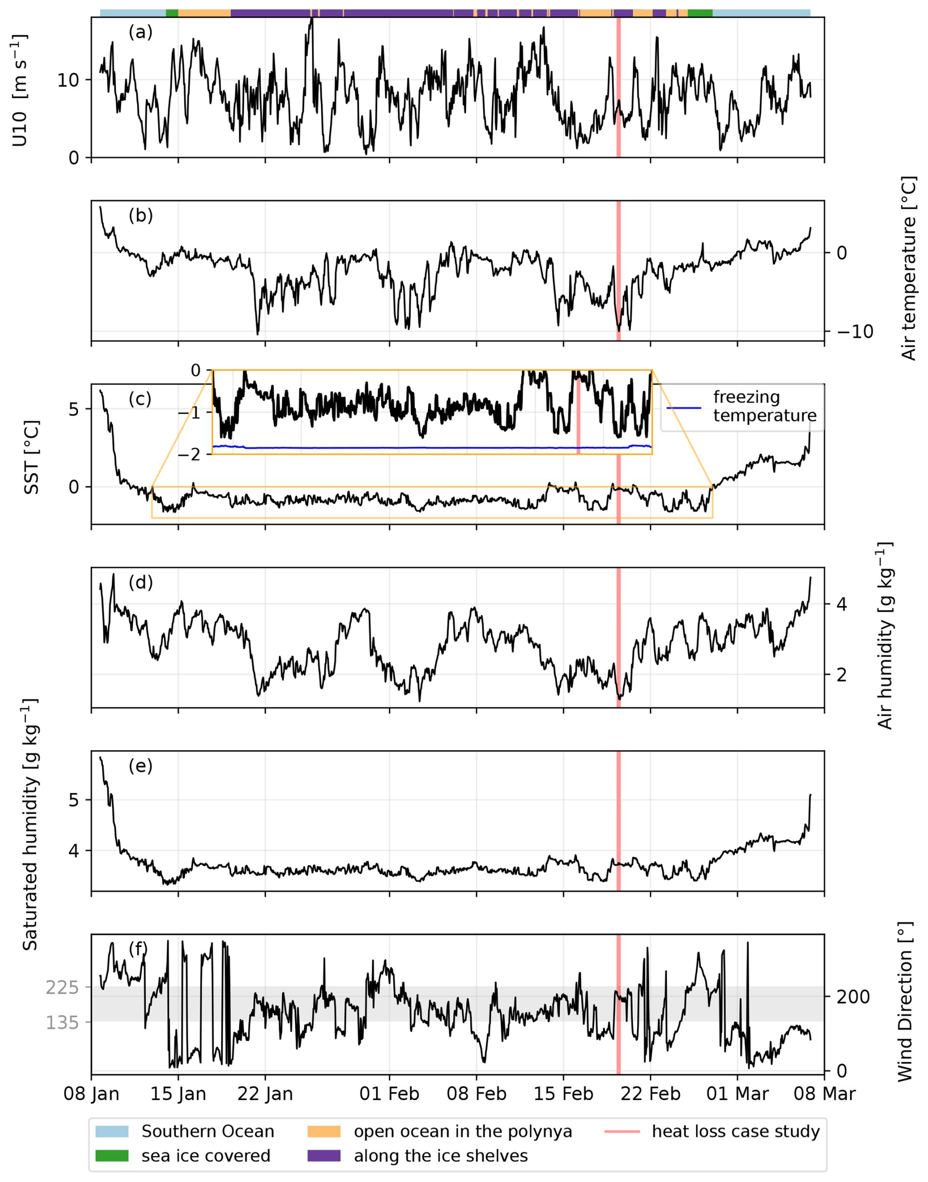
Figure 2 Main sea surface and atmospheric variables. The colors on top of the first time series are the classification of the position of the RV Nathaniel B. Palmer. Note that no sea ice was found near the ice-shelf front. The red area is the heat loss event selected for the case study (Sect. 3.1.3). The gray area in (f) represents the wind direction when blowing from 135 to 225°, i.e., blowing from the southwest, south, and southeast.

The Amundsen Sea (comprising the polynya region and along the ice shelves in the classification) lost on average more turbulent heat (−52 W m⁻², SD = 51 W m⁻²) than the Southern Ocean region (−30 W m⁻², SD = 26 W m⁻²; Fig. 3e). The largest instantaneous heat loss events were also observed in the Amundsen Sea (the maximum is −230 W m⁻² versus −145 W m⁻² in the Southern Ocean). In particular, more than 97 % of the turbulent heat loss events larger than 150 W m⁻² occurred when the ship was within 20 km of the Dotson or Getz ice shelves (purple classification, Fig. 3).

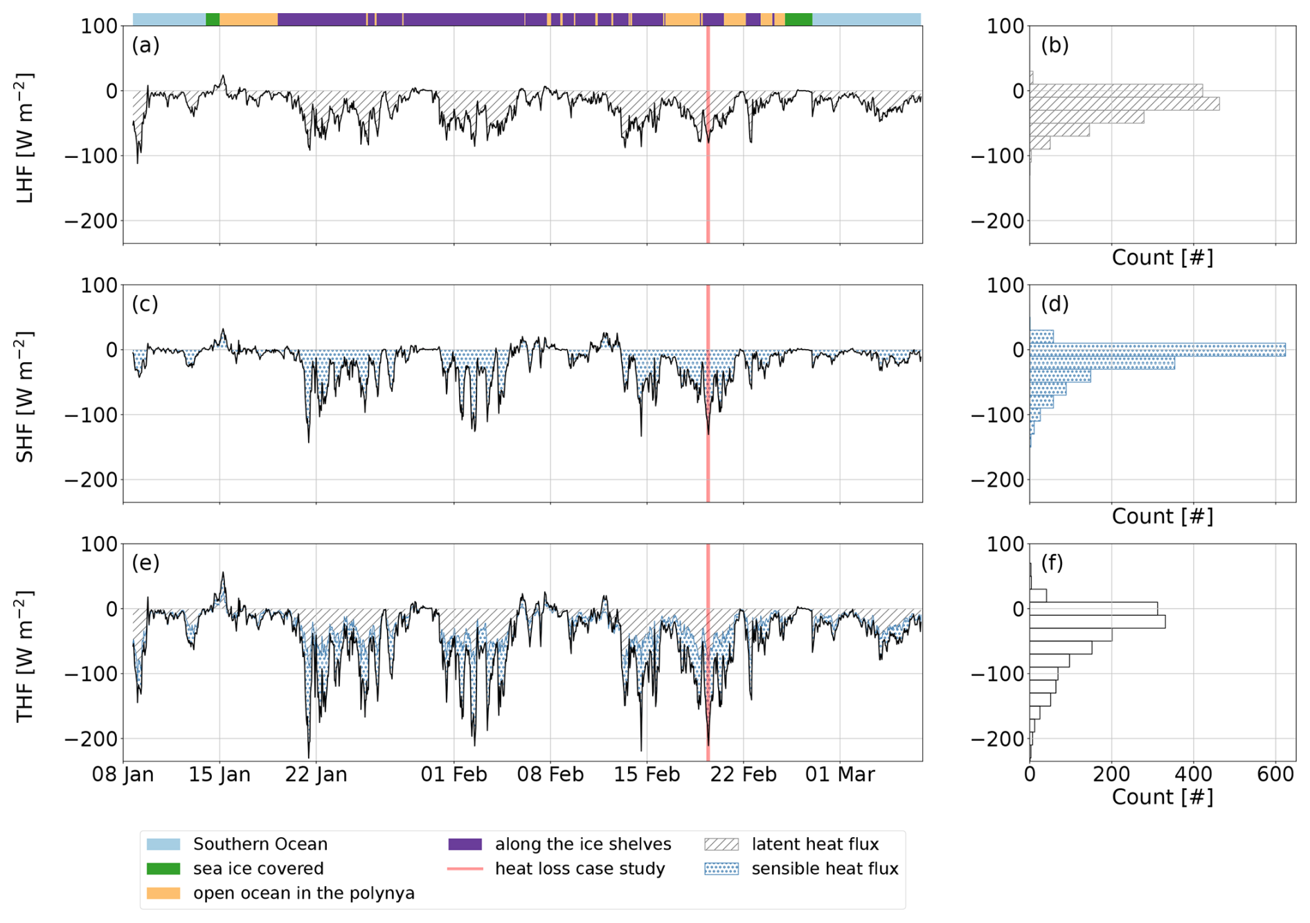
Figure 3 Ship observations of (a, b) latent heat flux, (c, d) sensible heat flux, and (e, f) the sum of the two: the turbulent heat flux. A positive heat flux is a gain by the ocean (downward convention). The colors on top of the first time series and the red area are as in Fig. 2.

Within the polynya region, the THF variations (Fig. 3e) were linked to short-scale SHF loss between −90 and −140 W m⁻² (Fig. 3c), while in the Southern Ocean, the largest turbulent heat loss events (Fig. 3e) were driven by the LHF loss (Fig. 3a).

Throughout the time series, the LHF contributed most to the net THF loss, accounting for an average of 57 % of the THF. This is evidenced by the mode of both the LHF and THF being between −30 and −10 W m⁻², whilst for the SHF, the mode is between −10 and 10 W m⁻² (Fig. 3b, d, f). Thus, while the LHF contributed the most to the total THF, the most significant short-term (days to weeks) THF loss events were imputed to large SHF losses.

3.1.2 Turbulent heat flux decomposition – enhanced air–sea temperature and humidity gradients responsible for large episodic heat loss events

Below, we investigate the key drivers of the variability in the THF. We decompose the flux anomalies into different terms (Eqs. 6, 7). These terms indicate the contributions to SHF^′ and LHF^′ of the temperature gradient (t term), humidity gradient (q term), wind speed (u term), transfer coefficients (ct term and cq term), and the cross-contribution of the following variables: second-order terms (t–u term, q–u term, u–cq term, etc.) and a third-order term or residual (covariance term) (Fig. 4).

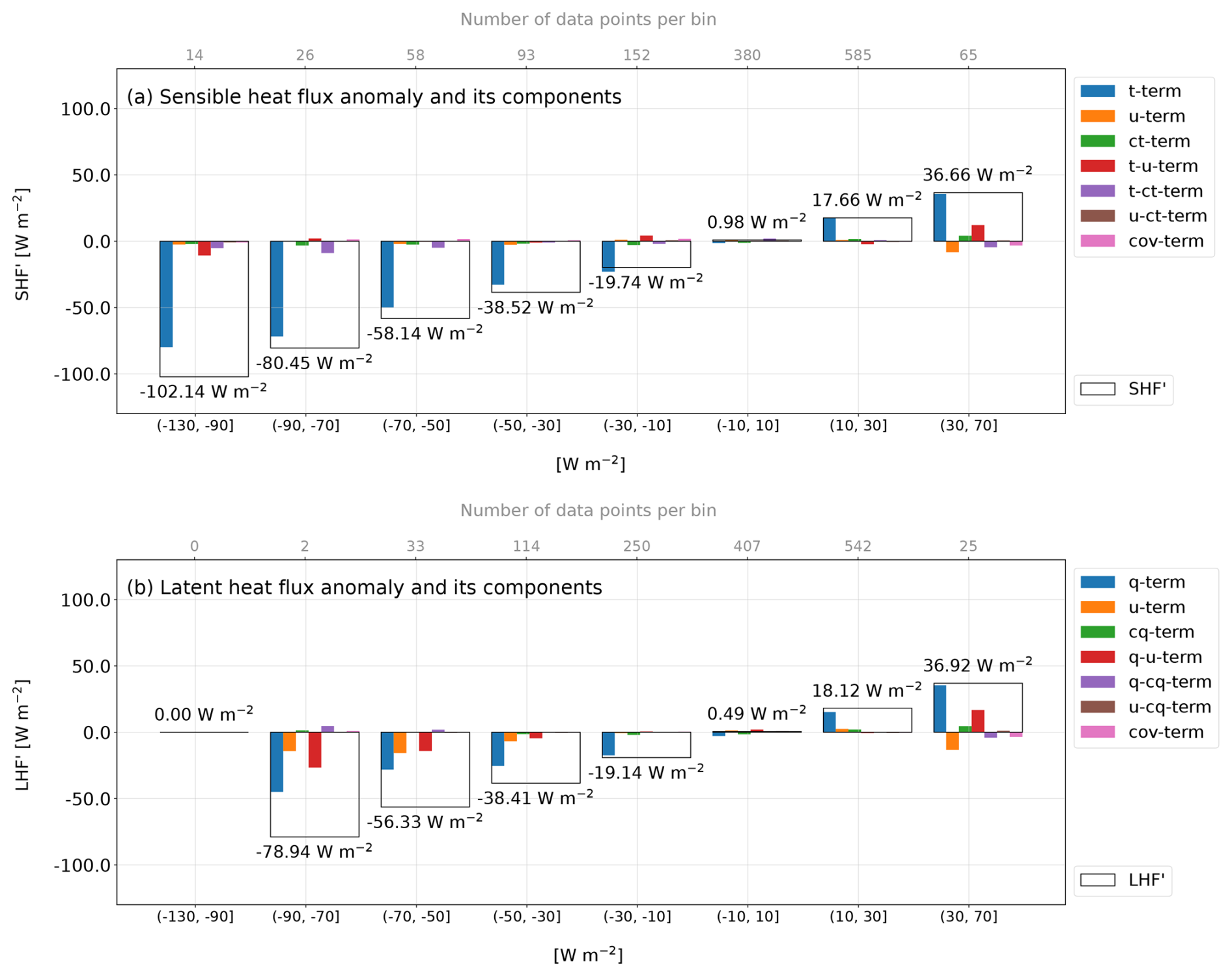
Figure 4 (a) Mean SHF^′ and (b) mean LHF^′ in black rectangles binned by 20 or 40 W m⁻² (for the first and the last bins). The numbers outside of the black rectangles are the mean values of the SHF^′ (a) and LHF^′ (b) for the corresponding bin. The colored bars inside the black rectangles are the different terms from Eqs. (6) and (7). Their sum gives SHF^′ and LHF^′.

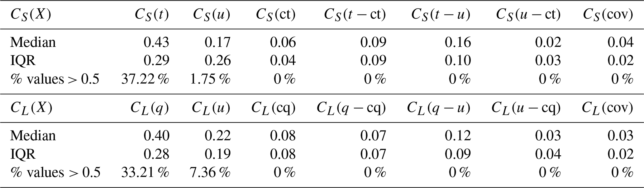
The t term (associated with the anomalous air–sea temperature gradient) was larger than the sum of all the other terms (Fig. 4a, blue color bars dominate). The indices of contribution of the terms (Table 3) were calculated for each hourly data point and range between 0 and 1 to show the relative importance of one term compared to another. The t term was the most frequent dominating factor: 37 % of C_S(t) values were above 0.5 (Table 3). This indicates that in 37 % of the data, air–sea temperature gradients were responsible for more than 50 % of SHF^′. Following the same arguments, the q term (the anomalous air–sea humidity gradient) contributed the most to LHF^′ (Fig. 4b, blue color bars) but to a slightly lesser extent: above 33 % of LHF^′ values had C_L(q) as the strict dominant factor.

Table 3 Median and interquartile range (IQR) of the indices of contribution for the seven terms of the Reynolds decomposition. C_L(X) is the contribution of the variable anomaly X to LHF^′; C_S(X) is the contribution of the variable anomaly X to SHF^′. An index of contribution higher than 0.5 means that the term is the strict dominant factor.

The decomposition indicates that the variability in the air–sea property gradient was the dominant factor impacting the variations in the THF. Further investigations show that the atmospheric variables (air temperature and humidity) control the air–sea property gradients. Indeed, the variability in the air temperature is higher (standard deviation (SD) = 2.62 °C) than the variability in the SST (SD = 1.13 °C; Fig. 2b, c). The same statement holds for the humidity: the air humidity has a higher variability (SD = 0.70 g kg⁻¹) than the saturated humidity (SD = 0.32 g kg⁻¹; Fig. 2d, e). The difference in SD is even larger when we remove the Southern Ocean data (not shown). These results indicate the importance of cold, dry air masses driving large heat loss events.

3.1.3 Case study of the heat loss mechanism in the Amundsen Sea – cold and dry southerlies trigger the heat loss

To further analyze the heat loss mechanism in the Amundsen Sea, we investigate the relationship between the turbulent heat loss and the broader-scale synoptic variability (Fig. 5).

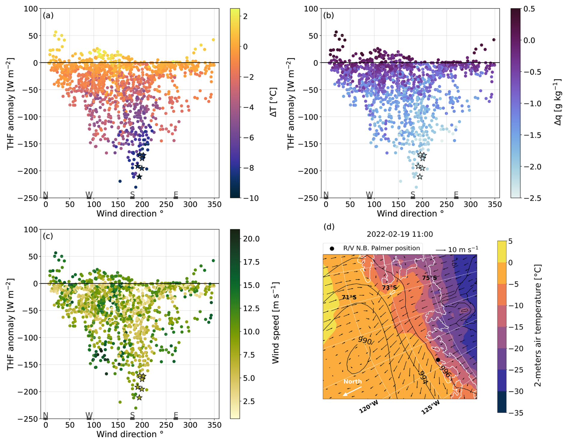
Figure 5 (a–c) THF plotted by the wind direction and colored according to (a) the temperature gradient, (b) the humidity gradient, or (c) the wind speed. The stars correspond to the heat loss event studied and depicted in (d). Panel (d) is the Amundsen Sea; the coastline is in white. The black dot is the research vessel position on 19 February 2022. The 10 m wind speed and direction (arrows), the 2 m air temperature (background), and the isobars (black contour) are plotted for the same day at 11:00 GMT and from ERA5.

The large turbulent heat losses were associated with winds blowing from the south (Fig. 5a, b, c), with large temperature (Fig. 5a) and humidity (Fig. 5b) gradients. We focus on one heat loss event that lasted 6 h on 19 February 2022 from 08:00 to 13:00 GMT (stars in Fig. 5). The THF remained below −170 W m⁻² (Fig. 3, red area), reaching its peak of −211 W m⁻² at 11:00 GMT. The mean value over the 6 h was −186 W m⁻². The wind was directed from the continent (Fig. 5d wind vectors and Fig. 2f) and brought cold (on average −9.4 °C; Fig. 2b) and dry (1.4 g kg⁻¹; Fig. 2d) air on top of the warmer (on average −0.1 °C; Fig. 2c) and moister (3.7 g kg⁻¹; Fig. 2e) sea, triggering the heat loss event. A low-pressure center was also visible on the map (Fig. 5d). It may have enhanced the heat loss event. This weather system (cold and dry continental winds) has been observed for all the major turbulent loss events occurring during this research cruise (not shown). On the contrary, the instances when the THF was significantly positive (> 30 W m⁻²) are consistent with warm and moist northerlies blowing over the Amundsen Sea (Figs. 3e and 2f).

This indicates the role of large-scale atmospheric variability on the local flux events. Next, we review the state-of-the-art reanalysis to understand the ability of numerical weather models to represent these key processes.

3.2 ERA5 reanalysis – revealing the product bias in the Amundsen Sea

3.2.1 Turbulent heat flux bias at land–sea boundaries

The research vessel spent 72 % of its time in the polynya region and along the Dotson and Getz ice shelves, where few validations of ERA5 have been conducted. First, we analyze the THF from ERA5 by comparing it to the observed fluxes, which were calculated using the COARE 3.5 algorithm (Fig. 6).

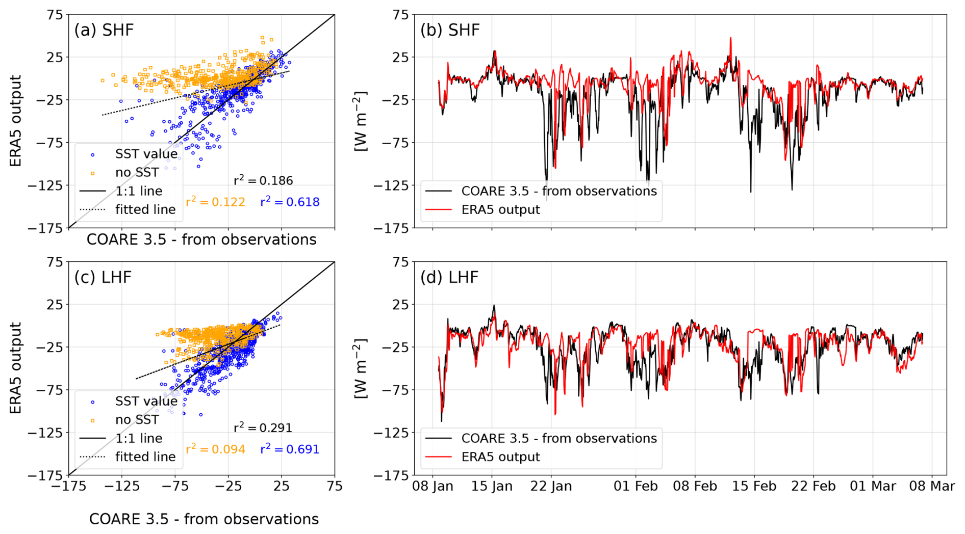
Figure 6 (a, b) SHF and (c, d) LHF. Panels (a) and (c) are colored by an SST mask (the data points where the ERA5 cell has an SST value are in blue, and where SST is NaN (not a number), the data points are in yellow: these points are then classed as ice shelf). The r² in black is the coefficient of determination for all the data points; the r² in blue and in yellow are the coefficients of determination of the data points corresponding to the SST mask. (b, d) The black lines are the fluxes computed from the research vessel measurements using the COARE 3.5 algorithm; fluxes from ERA5 are in red. ERA5 fluxes are co-located to the research vessel position by selecting the nearest ERA5 value.

The agreement between the THF product from ERA5 and the THF calculated from in situ data via COARE 3.5 was low: r² = 0.186 for the SHF (Fig. 6a) and r² = 0.291 for the LHF (Fig. 6c). Additionally, ERA5 was positively biased in comparison to the observations: the mean SHF and LHF were higher by 13 and 3 W m⁻² (Table 4, first and second rows). Similarly, hourly episodic heat loss events were not well represented by ERA5 (Fig. 6b, d): the difference between the two time series was up to 141 W m⁻² for the SHF and 81 W m⁻² for the LHF (Table 4, second row).

Table 4 Comparison of the different flux products. The LHF and SHF max diff. are the maximum absolute differences between the flux from the in situ observations and from another flux product (either the ERA5 fluxes or the ERA5 hybrid fluxes). RMSE is the root-mean-square error.

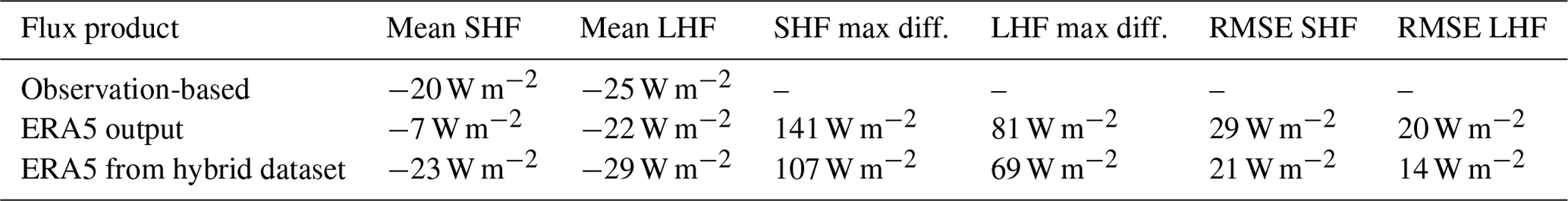
The low agreement between the two flux products is explained by the coarse resolution of ERA5 at land–sea boundaries. The research vessel was often stationed along the ice shelves where the closest ERA5 grid cell was considered ice shelf and as such does not have an SST value (Fig. 7). The correlation between ERA5 and the COARE 3.5 fluxes improved when only comparing instances where the nearest ERA5 grid cell had an SST value not set to NaN (not a number) (r² = 0.618 for the SHF and r² = 0.691 for the LHF; Fig. 6a and c, blue points). For instances where there is no SST, the correlation is weak (r² = 0.122 for the SHF and r² = 0.094 for the LHF; Fig. 6a and c, yellow points). Thus, the ERA5 reanalysis THF product underestimates the turbulent losses at the land–sea boundary formed by the ice shelves due to missing SST values. These results illustrate the importance of careful analysis when investigating ice-shelf processes in reanalyses.

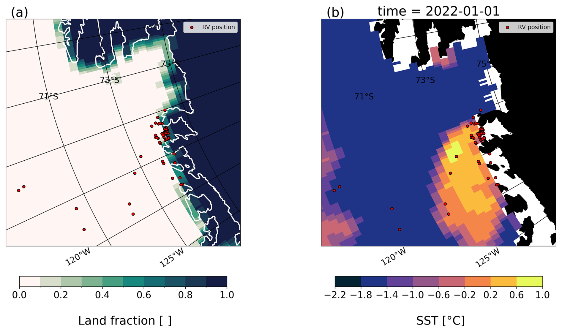
Figure 7 (a) Land–sea mask from ERA5 and (b) SST from ERA5. The research vessel position is plotted every 18 h (red data points).

3.2.2 A hybrid dataset to reduce the bias

As shown above, the dominant mechanism impacting the THF was the variations in air temperature and humidity. As such, to make use of all available ship-based observations to compare with ERA5, we require a more suitable method to reduce the SST-based biases identified. We considered using the nearest THF that is an ocean point, but this method was not chosen, as this would introduce a bias into the THF magnitude caused by an overestimation of air temperature (not shown).

We create an ERA5 dataset with the atmospheric variables (wind, air temperature, dewpoint temperature, pressure) co-located using the closest ERA5 value and with the SST co-located using the closest cell that has an SST value. We found this reasonable, as the SST variability is less important (range = 1.9 °C) than the air temperature (range = 12.2 °C) in the polynya region during the research cruise (Fig. 2b, c). Therefore the gradient of temperature in Eq. (1) mainly depends on the air temperature. The COARE 3.5 algorithm was then applied to compute turbulent fluxes using the new dataset as input (Fig. 8). We refer to the original ERA5 THF product as the nearest-neighbor product, which suffers from an inaccurate landmass, and the new product calculated from the ERA5 atmospheric variables and valid SST as the hybrid product (hybrid because of the differences in the co-location method between the SST and the other variables).

Figure 8 (a, b) SHF and (c, d) LHF from the COARE 3.5 algorithm with input from the ERA5 hybrid dataset (in red) and input from RV Nathaniel B. Palmer measurements (in black).

The SHF correlation between ERA5 and the observations was higher with the ERA5 hybrid dataset (r² = 0.576; Fig. 8a) than the original nearest-neighbor dataset (r² = 0.186; Fig. 6a). The same statement holds for the LHF: r² = 0.658 for the hybrid dataset (Fig. 8c) versus r² = 0.291 for the nearest-neighbor flux (Fig. 6c). The hybrid SHF was on average closer to the observation-based fluxes (lower by 3 W m⁻²; Table 4) but with a negative bias because of colder air temperature (Fig. D1c). Regarding the mean LHF, the hybrid dataset did not bring a clear improvement: the mean hybrid SHF is lower by 4 W m⁻² than the SHF from observations, whereas the mean ERA5 SHF output was higher by 3 W m⁻². The instantaneous heat loss was slightly better represented (Fig. 8b, d in comparison to Fig. 6b, d), with a maximum difference between the time series of 107 W m⁻² for the SHF and 69 W m⁻² for the LHF (Table 4).

3.3 1D model simulations and glider data – determining the importance of an accurate turbulent heat flux estimate

We presented the characteristics of the heat loss events in the Amundsen Sea (Sect. 3.1) and evaluated ERA5 in this region (Sect. 3.2). We found an underestimation of the turbulent heat loss from ERA5 THF output, and we created a hybrid ERA5 dataset that overestimates the heat loss but fits the observations better. In this last section we evaluate the impact of the THF on the SST and HC variability. More specifically, we determine whether the overestimation (or underestimation) of ERA5 fluxes is critical for estimates of SST and HC. We use a 1D model to answer these questions. We ran four PWP simulations with different atmospheric forcing that differed only in their THFs (Figs. C2e, g and 9a). Out of the four THF products, three were used earlier in this study: the THF computed from the research vessel via COARE 3.5 (observation dataset), the ERA5 THF co-located using the nearest-neighbor approach (suffering from the land-mask issue), and the THF computed from the ERA5 hybrid dataset via COARE 3.5. The last THF is obtained directly from ERA5 at a single ocean grid cell so as to represent the time-varying dynamics and exclude any lateral processes associated with a moving ship. We call this the stationary dataset.

3.3.1 Turbulent heat flux effect on sea surface temperature

The PWP model predicted a warming of the water column over the 35 d for all four simulations (Fig. 9g), which is in agreement with the seasonal warming expected during the austral summer. However, the SSTs of the four PWP simulations diverge (Fig. 9c). At the end of the 35 d run (the duration of the expedition in the polynya region), the nearest-neighbor SST (yellow line) was higher (0.76 °C; Fig. 9e) than in the other three simulations. The hybrid (blue line) and stationary (pink line) simulations were colder (−0.17 and −0.14 °C) than the observation simulation (dark-green line in Fig. 9c). This is in agreement with the ERA5 overestimation of heat loss for the hybrid dataset and underestimation for the nearest-neighbor dataset. The HC in the 40 m upper layer was higher by 8.2 × 10⁷ J at the end of the 35 d for the nearest-neighbor simulation and lower by −3.30 × 10⁷ and −2.98 × 10⁷ J for the hybrid and stationary simulations (Fig. 9f) in comparison to the observation-based simulation.

Figure 9 (a) THF input for the PWP model. (b) THF difference for the observation-based simulation minus one of three other simulations. (c) SST model output and (d) HC in the upper 40 m layer computed from the model's output. Panels (e) and (f) are the differences in SST and HC between the observation-based run and the other runs. Panel (g) shows the initial temperature profile (dotted line) and the final temperature profiles. The gray-shaded area in all the panels corresponds to a 2 d period that we examine in the results.

The observation and the nearest-neighbor simulations had large THF differences (on average 28 W m⁻² and instantaneously up to 200 W m⁻²; Fig. 9b, yellow points) that led to an increase in the slope of the difference in SST (Fig. 9e) and HC (Fig. 9f) between the two simulations. For example, from day 13.5 to day 15.5 (gray-shaded area), the nearest-neighbor THF was on average 82 W m⁻² warmer than the observed THF. This difference explained an SST increase of 0.20 °C and an HC increase of 1.4×10⁷ J (yellow line; Fig. 9e, f) in the nearest-neighbor simulation in comparison to the observation-based simulation. The cumulative effect of such events is critical to set the SST and HC differences between the simulations throughout the 35 d simulations (Fig. 9e, f).

We note that the daily change in SST (ΔSST; Table 5) has the same order of magnitude between the stationary-dataset-based simulation (mean = 0.003 °C d⁻¹, SD = 0.042 °C d⁻¹) and the hybrid-dataset-based simulation (mean = 0.002 °C d⁻¹, SD = 0.040 °C d⁻¹), which gives us confidence in the credibility of using the PWP model with data that are not stationary (i.e., biases introduced when comparing datasets from moving vessels).

Thus, the four simulations diverge because of the different THF inputs (indeed all the other atmospheric forcings are identical). The resulting difference in evolution of SST (HC) of 0.76 °C (8.2 × 10⁷ J) over a month is not negligible for a coastal polynya region where sea-ice formation and melting, ice-shelf melting and primary production are dominant processes.

3.3.2 A sea surface temperature and heat content bias as large as the spatial-scale variability

In this final subsection, we look at ship-based thermosalinograph (TSG) data (for the SST) and nearby glider data (for the HC) to understand how the temperature change in the PWP simulations compares to the change in temperature in the observations.

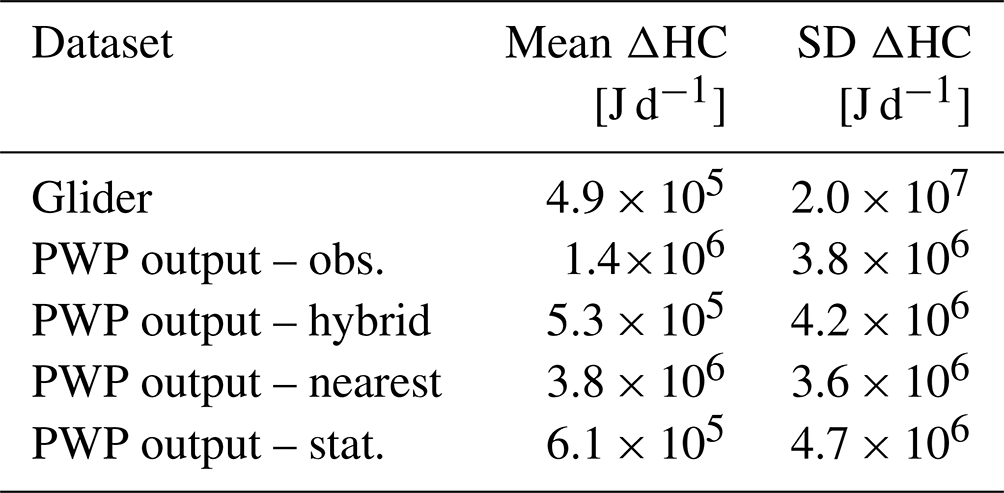
ΔSST from the PWP model output (solid lines, Fig. 10a) and from the TSG observations (dotted line) showed a similar average change (Table 5; mean = O(10⁻³) °C d⁻¹), except for the nearest-neighbor PWP output, which has a higher mean (0.029 °C d⁻¹). Regarding the HC, the nearest-neighbor simulation exhibits a higher mean as well, even though the difference is smaller than for the SST (Table 6). SDs of the daily change in SST and HC are 1 order of magnitude higher for the observations (0.140 °C d⁻¹, 2.0 × 10⁷ J d⁻¹) than for the model outputs (O(10⁻²) °C d⁻¹, O(10⁶) J d⁻¹; Tables 5 and 6). The larger spread in the observations can be explained by the horizontal processes that are assumed to be non-negligible in a sea-shelf environment and that were not represented in the 1D model.

It is thus reasonable to assume that the horizontal processes average out (as seen by the comparison of the means); the 35 d evolution of SST and HC in the observations was well represented by the PWP simulations when the nearest-neighbor simulation was set aside.

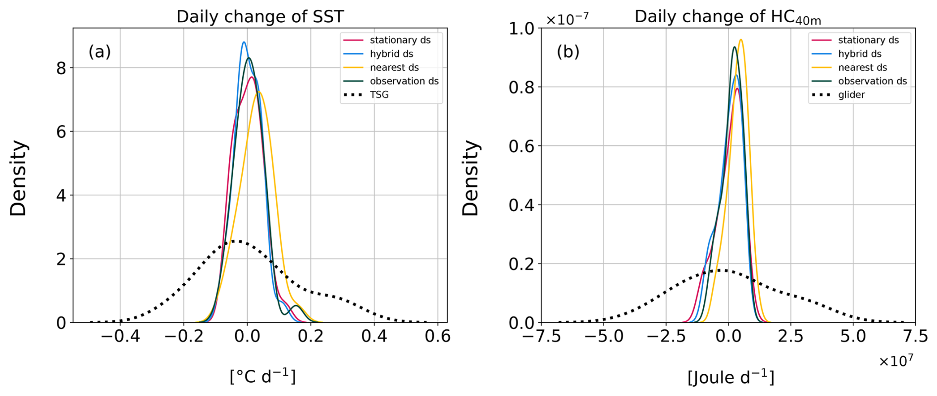
Figure 10 Distribution of (a) the daily change in SST and (b) the daily change in HC in the upper 40 m layer for the four PWP simulations (continuous line) and the observations (dotted line). For the observations, we used ship-based data at 6 m for the SST and glider data for the HC.

Table 5 Statistics of the change in temperature $\mathrm{\Delta }\mathrm{SST}={\mathrm{SST}}_{t_{i+\mathrm{1}}}-{\mathrm{SST}}_{t_i}$, with $t_{i+\mathrm{1}}-t_i=\mathrm{1}$ d. SD is the standard deviation. The SST is taken at a depth of 6 m for the PWP model to match the depth of the TSG measurements.

Table 6 Same as the previous table but for statistics of the daily change in heat content in the upper 40 m layer.

Coming back to the 2 d example of the previous section, according to the PWP model, we see a misrepresentation of the THF of about 80 W m⁻² (Fig. 9b) that leads to an SST increase of 0.2 °C (Fig. 9e) and an HC increase of 1.4 × 10⁷ J (Fig. 9f). Across this particular heat loss event, the SST and HC increases were on the same order of magnitude as the spatiotemporal variability scale observed in the 35 d ship-based SST observation (SD = 0.140 °C d⁻¹; Table 5, Fig. 10a) and 18 d glider data (SD = 2.0 × 10⁷ J d⁻¹; Table 6, Fig. 10b) that were imputed to horizontal processes. Therefore, the cumulative effect of small differences in the mean ΔSST and ΔHC due to a bias in the THF is critical for the temporal-scale variability in SST and HC in the Amundsen Sea. The 1D processes alone cannot explain the change in SST and HC that we see in the observations. However, our work highlights the fact that a consequent bias in the THF can lead to errors in the estimation of the 35 d evolution of the SST and HC that are on the same order of magnitude as the variability due to horizontal processes.

4 Discussion and conclusions

This work provides the first air–sea THF-observation-based study in the Amundsen Sea. Large-scale cold and dry winds moving from the Antarctic continent over the sea enhance the air–sea temperature and humidity gradients and trigger turbulent heat loss events up to 230 W m⁻². We show that THFs from ERA5 are inaccurate at ice-shelf boundaries (mean underestimation of the heat loss of 28 W m⁻² over the 35 d of the research survey in the polynya region). This can be improved by recalculating fluxes from ERA5 sea surface and atmospheric variables, with vigilance regarding the SST that is sometimes set to NaN due to the ERA5 land–sea mask. The THF obtained overestimates the heat loss by 12 W m⁻² on average in the polynya region. As a result of misrepresenting the THF, we show that the seasonal evolution of the modeled SST would be overestimated (+0.76 °C at the end of the 35 d PWP simulation) with ERA5 THF or underestimated (−0.17 °C) with ERA5 recalculated flux. Therefore, caution has to be taken when selecting turbulent fluxes for modeling studies in a coastal polynya where, for example, sea-ice formation and melting and primary production are important processes.

4.1 Polynya turbulent flux system

4.1.1 The role of the broader atmospheric system

Antarctica is known for its strong surface winds. It might be plausible that the wind contributes significantly to the heat loss by increasing turbulent mixing, yet we did not observe any pattern of increasing wind intensity related to the heat loss (Figs. 4 and 5c). A systematic positive bias in the residuals was observed in Fig. A1, meaning that either ERA5 underestimates the wind speed or the measurements overestimate it. We imputed the residual bias to ERA5, as it has been shown that the wind speed along the Antarctic coastline is underestimated by ERA5 (Caton Harrison et al., 2022). The properties of the air (cold and dry) transported by the winds are more important for the THF variability than the wind speed itself. As shown, the atmospheric system is thought to be a key component in the Amundsen Sea. Indeed, Jones (2018) used the MetUM model to perform episodic (2 to 3 d) high-heat-flux case studies in the eastern Amundsen Sea and found that strong easterlies and southeasterlies associated with cyclones are typically linked to heat loss. The importance of low-pressure systems in cold-air outbreaks is a result that has also been found in the Ronne Polynya (Weddell Sea) from aircraft observations (Fiedler et al., 2010). The Amundsen Sea is known for being a cyclogenesis region, and we indeed saw recurring low-pressure centers in our study area (Fig. 5d). In particular, the Amundsen Sea Low (ASL) is a quasistationary low-pressure center that oscillates between the Ross Sea (to the west) and the Bellingshausen Sea (to the east). Hosking et al. (2013) showed that the ASL influences the meridional component of the large-scale atmospheric circulation. When the ASL is positioned to the west, it enhances the southerly flow. The ASL was located at the edge of the Ross and Amundsen seas (to the west) in January and March 2022 and in front of Thurston Island, in the Amundsen Sea, in February 2022 (the ASL index position was downloaded from https://github.com/scotthosking/amundsen-sea-low-index, last access: 31 January 2025). The ASL had, therefore, likely enhanced the southerly (continental) winds over the time span of the research vessel's presence in the Amundsen Sea and consequently increased the turbulent heat loss through enhanced air–sea temperature and humidity gradients. It would be interesting in future studies to investigate the longer-term air–sea THF variability associated with ASL location.

4.1.2 Spatial variability in the fluxes

In this study, the largest heat losses occurred in front of the ice shelves. This result could indicate that the heat loss is larger along the ice shelves than in the open water in the polynya but could also be explained by the fact that the research vessel spent 27 d out of 41 d in front of the ice shelves when in the polynya region. However, it has been shown by modeling studies in other coastal polynyas (Renfrew et al., 2002, for the polynya that forms off Ronne Ice Shelf (Weddell Sea) and Jones, 2018,  for the Pine Island Glacier Polynya, Pope Smith Kohler Polynya, and Thurston Polynya (eastern Amundsen Sea)) that the THF decreases with fetch. When continental cold (dry) air is advected on top of the sea, it gains heat (moisture) from the ocean as it travels offshore, which reduces the gradient of temperature (humidity) and, as a consequence, the SHF (LHF). This result gives us confidence regarding the spatial variability observed in our dataset and illustrates the key mechanisms for driving heat loss in regions of ice-shelf dynamics.

4.2 Assessing ECMWF turbulent heat flux in the Amundsen Sea

From ERA-Interim data, Papritz et al. (2015) created a CAO climatology. They found that the CAO summer frequency is under 3 % and consequently focused on the nonsummer months. In autumn, winter, and spring, they found that the CAOs contribute to the turbulent heat loss enhancement. Their study focused on the region of the Amundsen Sea off the ice shelves and therefore was not affected by the along-shelf dynamics assessed in our study. Yet, we found the same result regarding the importance of CAOs along the ice shelves, as the air was cold and dry enough to enhance the air–sea temperature and humidity gradients despite it being summertime. Jones et al. (2016) evaluated the performance of four reanalysis products in the Amundsen Sea and showed that ERA-Interim has a cold bias in the air temperature and a dry bias in the specific humidity, which are greater near the ice shelves and weaker far from the coast. As a consequence, they hypothesize that the heat loss would be overestimated. This hypothesis has been verified in our work, with the bias found (Table 4) in ERA5 hybrid fluxes (computed from the atmospheric and sea surface ERA5 variables). This bias indeed arises from cold and dry biases in ERA5 air and humidity (Fig. D1b, c). However, the ERA5 nearest-neighbor THF underestimates the heat loss: this result indicates the importance of careful choice regarding the method used to retrieve estimates of turbulent flux in the Amundsen Sea from ERA5.

4.3 Implications

The Amundsen Sea is a dynamic shelf sea with horizontal processes such as coastal currents. Therefore the 1D PWP model does not aim to reproduce the observed temperature changes. However, we use the PWP model to give an insight into the potential effects of an air–sea THF misrepresentation on the monthly evolution of SST in the Amundsen Sea. The stationary heat flux simulation and the hybrid simulation show similar results. This indicates that the large-scale nature of the CAOs, which drive the strongest fluxes, negates any bias that might have been induced by simulating a 1D model using flux data from a moving ship. In the nearest-neighbor simulation, which includes the strongly biased THF, there is a non-negligible impact on the overestimation of SST (+0.76 °C) and HC (8.2 × 10⁷ J) at the end of the 35 d simulation. Yu et al. (2023) have shown that the climatological January SST ranges between −0.8 and −0.2 °C in the Amundsen Sea Polynya (it has an internal spatial variability), with an interannual standard deviation between 0.35 and 0.45 °C. The SST from the hybrid, stationary, and observation simulations are therefore in the expected range, unlike the nearest-neighbor simulation (Fig. 9c). This could have a major impact on sea-ice-formation or primary production studies, as the sea-ice concentration variability is influenced by the SST in summer (Kumar et al., 2021), and the chlorophyll-a concentration is correlated with the SST in the Amundsen Sea (Garcia et al., 2021).

The Amundsen Sea Polynya has high rates of primary production that are driven by both the polynya duration and the iron supplied from melting ice shelves and glaciers (Arrigo et al., 2012). The polynya duration is the length of the open-water season. The sea-ice-retreat season (when the polynya opens) and advance season (when the polynya closes) are bound by a positive feedback loop: early sea-ice retreat in spring/summer implies more solar input at the sea surface since the albedo of seawater is lower than that of sea ice. More solar input subsequently leads to later and lower sea-ice formation in the advance season (autumn) (Nihashi and Ohshima, 2001; Stammerjohn et al., 2012). It is worth noting that 2022, when the in situ data of this study were collected, was a year of record-breaking-low summer Antarctic sea-ice extent (even though this record was then broken in 2023; Purich and Doddridge, 2023). Turner et al. (2022) and Yadav et al. (2022) showed that a deep ASL in spring associated with the Southern Annular Mode in a positive phase enhanced the sea-ice melting during this anomalously low summer sea-ice year. However the effect of the ASL on the air–sea fluxes is twofold and opposite. On one hand, a deeper ASL enhances the southerly flow, pushing the sea ice away from the shore, widening the polynya, and therefore allowing more shortwave radiation to enter the upper ocean, leading to radiative heat gain by the ocean. While on the other hand, we show in our study that the southerly winds bring cold and dry continental air, leading to turbulent heat loss. While the main component of the net air–sea heat flux in summer remains the radiative heat flux, we show that synoptic-scale events can set in motion large episodic turbulent fluxes that reduce the net heat flux. Given that the Antarctic sea ice seems to have reached a new state in recent years (Purich and Doddridge, 2023), it is important to deepen our understanding of the complex atmosphere–ice–sea system. For instance, Stewart et al. (2019) show near the Ross Sea Polynya that the ice-shelf basal melting from surface heating is more important than what was traditionally thought, and it is expected to increase in the future. Based on our results, we propose that the dynamics controlling turbulent heat fluxes in these climate-sensitive regions should be considered as well.

4.4 Outlook

A number of potential avenues of work became clear during the course of this study. (i) As mentioned earlier, it would be interesting to have THF observations when the ASL is further east, to better understand the dependence of flux variability on the ASL. This corresponds to the austral winter or autumn (Hosking et al., 2016), seasons where we currently lack observations. (ii) The air–sea heat flux is the sum of the turbulent and the radiative components. We hypothesize that the bias in ERA5 THF induced by the land–sea boundary would affect the radiative fluxes as well, with a misrepresentation of the albedo. (iii) Finally, we could expect numerical models with higher spatial resolution than ERA5 to better capture the THF magnitude and variability along the ice shelves. We could, therefore, compare the observations to some high-resolution regional climate models (e.g., MetUM, RACMO) to evaluate their accuracy on a coastal shelf sea such as the Amundsen Sea.

Appendix A: Data processing – investigating the wind distortion effects

The anemometers on a ship can be positioned in a place where they experience airflow distortion from the superstructure of the research vessel (Yelland et al., 1998; Moat et al., 2005; Landwehr et al., 2020). The consequence is a bias in the wind speed values that depends on the location of the anemometers and the shape of the research vessel (Moat et al., 2005). We use ERA5 to analyze the residuals (i.e., the research vessel minus ERA5 wind speed) and to validate the in situ wind measurements (Fig. A1).

We observe a decreasing residual with wind blowing from the stern, which could be explained by the openness of the superstructure over the back half of the ship (Fig. A1b). The residuals are positive for each bin; this is possibly an overestimate of the measured wind speed but could also be a bias from ERA5. We assume that the bias is from ERA5, as it has been shown that it is biased low along the Antarctic coast (Caton Harrison et al., 2022). The mean residuals (blue lines, Fig. A1a) are low: the minimum is 0.40 m s⁻¹ for the bin (120, 135]°, and the maximum is 1.70 m s⁻¹ for the bin (0, 15]° (winds blowing from the bow); we therefore decide to keep the data, as the bias is not large.

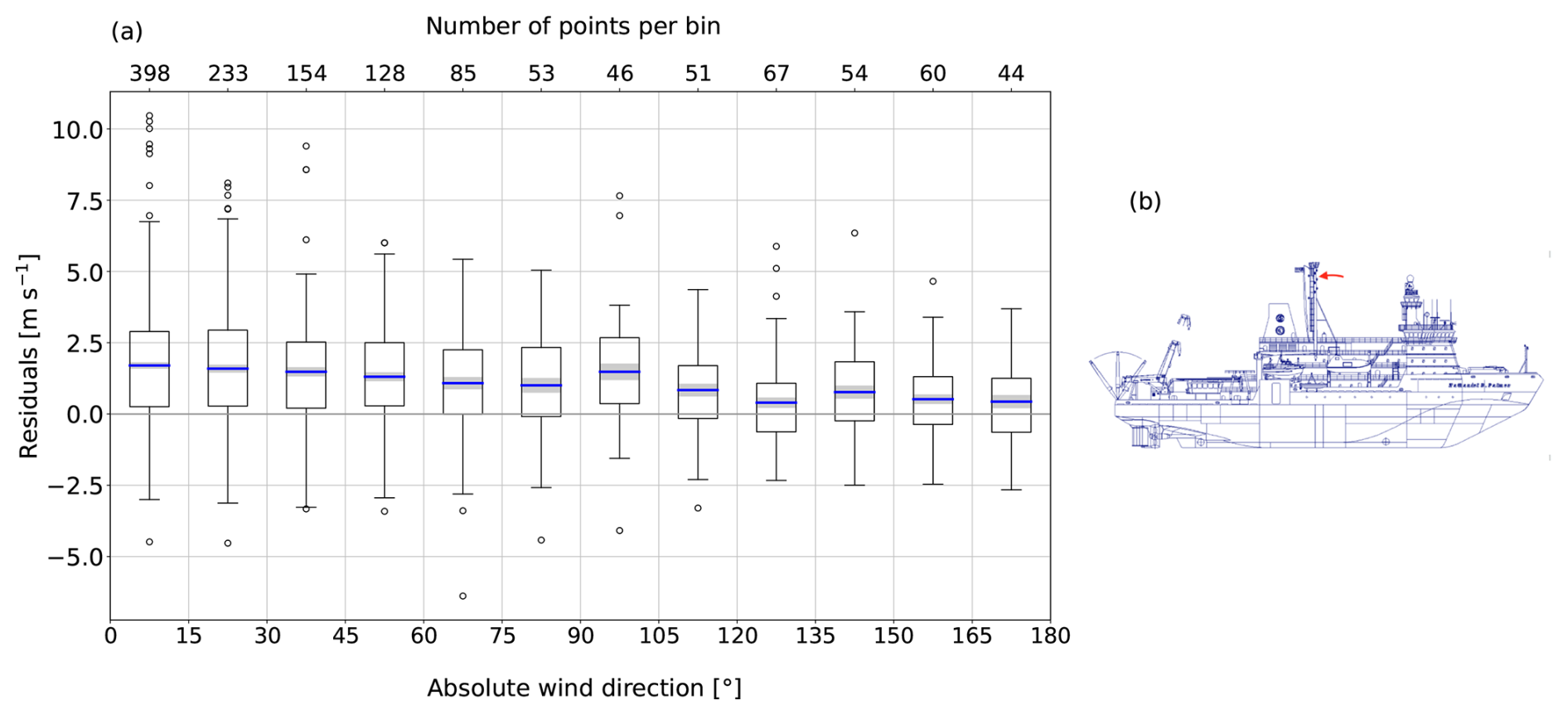
Figure A1 (a) Residuals (10 m wind speed[ship minus ERA5]) binned into 15° relative absolute wind direction. Relative means relative to the ship; the convention is the following: a 0° relative wind direction means the wind is blowing bow-on. Absolute refers to the assumption that the flow is symmetrically distorted on the port and starboard sides; e.g., the wind coming from (75, 90]° and from (−90, −75]° is distorted in the same way and is therefore placed into the same bin. The boxes extend from the lower to the upper quartile values, the whiskers represent the range of the data, and the black empty circles are outliers. The outliers are defined as data points lying outside the interval [Q1 − 1.5(Q3–Q1), Q3 + 1.5(Q3–Q1)]. The blue lines are the mean per bin. The gray-shaded areas indicate the standard error in the mean. Panel (b) is RV Nathaniel B. Palmer (adapted from https://www.usap.gov/USAPgov/vesselScienceAndOperations/documents/NBP_Guide.pdf, last access: 31 January 2025); the red arrow indicates the position of the anemometers.

Appendix B: Reynolds decomposition

The Reynolds decomposition consists of the decomposition of a variable X into the sum of its average ($\stackrel{\mathrm{‾}}{X}$) and anomaly (X^′). We applied this decomposition to the turbulent flux; the following are the mathematical steps that led to the formulation of Eqs. (6) and (7).

$$\begin{array}{}\text{(B1)}& {\displaystyle }\mathrm{SHF}={\mathit{\rho }}_{\mathrm{air}}{C}_{\mathrm{p}}(\stackrel{\mathrm{‾}}{C_{\mathrm{t}}}+C_{\mathrm{t}}^{\prime })(\stackrel{\mathrm{‾}}{U}+U^{\prime })(\stackrel{\mathrm{‾}}{\mathrm{\Delta }T}+\mathrm{\Delta }{T}^{\prime })\text{(B2)}& {\displaystyle }\mathrm{LHF}={\mathit{\rho }}_{\mathrm{air}}{L}_{\mathrm{v}}(\stackrel{\mathrm{‾}}{C_q}+C_q^{\prime })(\stackrel{\mathrm{‾}}{U}+U^{\prime })(\stackrel{\mathrm{‾}}{\mathrm{\Delta }q}+\mathrm{\Delta }{q}^{\prime })\end{array}$$

We expand these equations and average them (overline). We use the following averaging rules:

$$\begin{array}{}\text{(B3)}& {\displaystyle }\stackrel{\mathrm{‾}}{X^{\prime }}=\mathrm{0}\text{(B4)}& {\displaystyle }\stackrel{\mathrm{‾}}{\stackrel{\mathrm{‾}}{X}\stackrel{\mathrm{‾}}{Y}}=\stackrel{\mathrm{‾}}{X}\stackrel{\mathrm{‾}}{Y}\text{(B5)}& {\displaystyle }\stackrel{\mathrm{‾}}{\stackrel{\mathrm{‾}}{X}{Y}^{\prime }}=\stackrel{\mathrm{‾}}{X}\stackrel{\mathrm{‾}}{Y^{\prime }}=\stackrel{\mathrm{‾}}{X}\times \mathrm{0}=\mathrm{0}.\end{array}$$

We obtain

$$\begin{array}{}\text{(B6)}& {\displaystyle }\begin{array}{rl}\stackrel{\mathrm{‾}}{\mathrm{SHF}}& ={\mathit{\rho }}_{\mathrm{air}}{C}_{\mathrm{p}}[\stackrel{\mathrm{‾}}{C_{\mathrm{t}}}\stackrel{\mathrm{‾}}{U}\stackrel{\mathrm{‾}}{\mathrm{\Delta }T}+\stackrel{\mathrm{‾}}{C_{\mathrm{t}}}\stackrel{\mathrm{‾}}{U^{\prime }\mathrm{\Delta }{T}^{\prime }}+\stackrel{\mathrm{‾}}{U}\stackrel{\mathrm{‾}}{C_{\mathrm{t}}^{\prime }\mathrm{\Delta }{T}^{\prime }}\\ & +\stackrel{\mathrm{‾}}{\mathrm{\Delta }T}\stackrel{\mathrm{‾}}{U^{\prime }\mathrm{\Delta }{C}_{\mathrm{t}}^{\prime }}+\stackrel{\mathrm{‾}}{\mathrm{\Delta }{T}^{\prime }{C}_{\mathrm{t}}^{\prime }{U}^{\prime }}]\end{array}\text{(B7)}& {\displaystyle }\begin{array}{rl}\stackrel{\mathrm{‾}}{\mathrm{LHF}}& ={\mathit{\rho }}_{\mathrm{air}}{L}_{\mathrm{v}}[\stackrel{\mathrm{‾}}{C_q}\stackrel{\mathrm{‾}}{U}\stackrel{\mathrm{‾}}{\mathrm{\Delta }q}+\stackrel{\mathrm{‾}}{C_q}\stackrel{\mathrm{‾}}{U^{\prime }\mathrm{\Delta }{q}^{\prime }}+\stackrel{\mathrm{‾}}{U}\stackrel{\mathrm{‾}}{C_q^{\prime }\mathrm{\Delta }{q}^{\prime }}\\ & +\stackrel{\mathrm{‾}}{\mathrm{\Delta }q}\stackrel{\mathrm{‾}}{U^{\prime }\mathrm{\Delta }{C}_q^{\prime }}+\stackrel{\mathrm{‾}}{\mathrm{\Delta }{q}^{\prime }{C}_q^{\prime }{U}^{\prime }}]\end{array}.\end{array}$$

We then subtract the averaged $\stackrel{\mathrm{‾}}{\mathrm{SHF}}$ ($\stackrel{\mathrm{‾}}{\mathrm{LHF}}$) from the total SHF (LHF) to retrieve the anomalous SHF^′ (LHF^′) of Eq. (6) (Eq. 7).

Appendix C: PWP model input

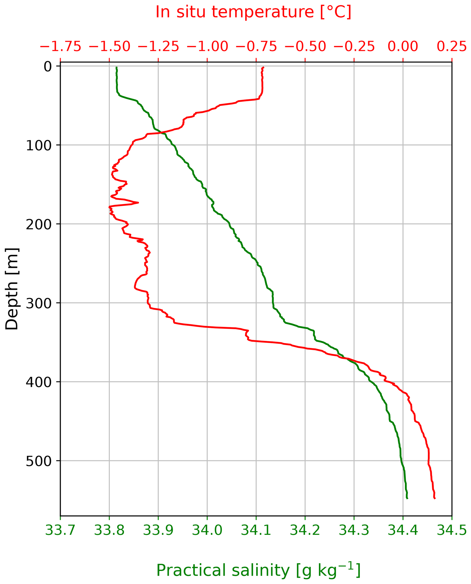
Figure C1 Oceanic forcing – initial temperature and salinity profiles for the PWP simulations from the CTD cast taken at 74.02° S, 113° W.

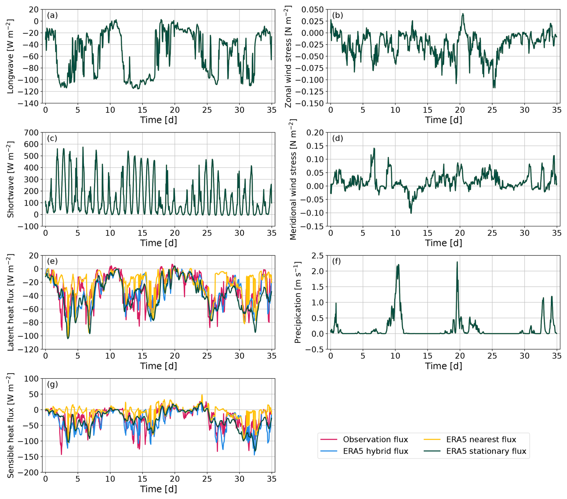
Figure C2 Atmospheric forcing – four runs were performed; only the latent and sensible heat fluxes differ. The shortwave, longwave, and wind stress come from the research vessel observations. The precipitation comes from the ERA5 stationary dataset because there was no observation of precipitation from the research vessel.

Appendix D: Comparison of in situ observations and ERA5 sea surface variables

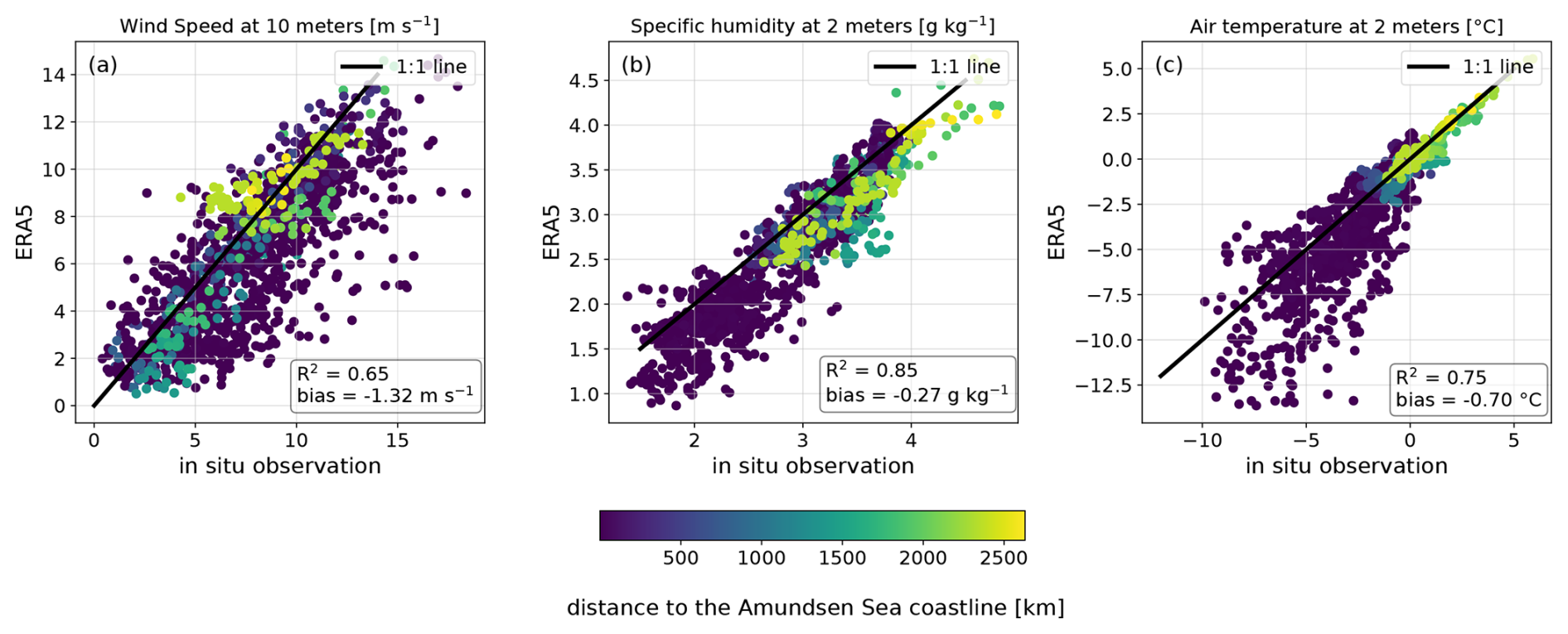
Figure D1 Comparison of (y axis) ERA5 and (x axis) in situ observations for (a) wind speed at 10 m, (b) specific humidity at 2 m, and (c) air temperature at 2 m. The in situ observations were adjusted down to 10 and 2 m, thanks to AirSeaFluxCode, which applies a logarithmic adjustment and stability functions to account for atmospheric stability. To determine specific humidity from ERA5, we convert the dewpoint temperature to specific humidity using the saturation vapor pressure function from Buck (2012). The points are colored according to the distance to the Amundsen Sea coastline in kilometers, which we defined as the closest coastal point to the ship position in the region 73.66–75.27° S, 108.10–122.64° W.