Benefits of a second tandem flight phase between two successive satellite altimetry missions for assessing instrumental stability

Five successive reference missions, TOPEX/Poseidon, Jason-1, Jason-2, Jason-3, and more recently Sentinel-6 Michael Freilich, have ensured the continuity and stability of the satellite altimetry data record. Tandem flight phases have played a key role in verifying and ensuring the consistency of sea level measurements between successive altimetry reference missions and thus the stability of sea level measurements. During a tandem flight phase, two successive reference missions follow each other on an identical ground track at intervals of less than 1 min. Observing the same ocean zone simultaneously, the differences in sea level measurements between the two altimetry missions mainly reflect their relative errors. Relative errors are due to instrumental differences related to altimeter characteristics (e.g., altimeter noise) and processing of altimeter measurements (e.g., retracking algorithm), precise orbit determination, and mean sea surface. Accurate determination of systematic instrumental differences is achievable by averaging these relative errors over periods that exceed 100 d. This enables for the precise calibration of the two altimeters. The global mean sea level offset between successive altimetry missions can be accurately estimated with an uncertainty of about ±0.5 mm ([16 %–84 %] confidence level). Nevertheless, it is only feasible to detect instrumental drifts in the global mean sea level exceeding 1.0 to 1.5 mm yr⁻¹ due to the brief duration of the tandem phase (9 to 12 months). This study aims to propose a novel cross-validation method with a better ability to assess the instrumental stability (i.e., instrumental drifts in the global mean sea level trends). It is based on the implementation of a second tandem flight phase between two successive satellites a few years after the first one. Calculating sea level differences during the second tandem phase provides an accurate evaluation of relative errors between the two successive altimetry missions. With a second tandem phase that is long enough, the systematic instrumental differences in sea level will be accurately reevaluated. The idea is to calculate the trend between the systematic instrumental differences made during the two tandem phases. The uncertainty in the trend is influenced by the length of each tandem phase and the time intervals between the two tandem phases. Our findings show that assessing the instrumental stability with two tandem phases can achieve an uncertainty below ±0.1 mm yr⁻¹ ([16 %–84 %] confidence level) at the global scale for time intervals between the two tandem phases that are higher than 4 years or more and where each tandem phase lasts at least 4 months. On regional scales, the gain is greater, with an uncertainty of ±0.5 mm yr⁻¹ ([16 %–84 %] confidence level) for spatial scales of about 1000 km or more. With regard to the scenario foreseen for the second phase between Jason-3 and Sentinel-6 Michael Freilich planned for early 2025, 2 years and 9 months after the end of the first tandem phase, the instrumental stability could be assessed with an uncertainty of ±0.14 mm yr⁻¹ on the global scale and ±0.65 mm yr⁻¹ for spatial scales of about 1000 km ([16 %–84 %] confidence level). In order to achieve a larger benefit from the use of this novel cross-validation method, this involves regularly implementing double tandem phases between two successive altimetry missions in the future.

1 Introduction

The altimetry sea level data record has been continuously calculated using multiple satellite altimetry missions since January 1993. The five successive reference missions, TOPEX/Poseidon (TP), Jason-1, Jason-2, Jason-3, and more recently Sentinel-6 Michael Freilich (S6-MF), have ensured the continuity and stability of the sea level data record. The upcoming launches of the Copernicus Sentinel-6B and Sentinel-6C satellites in the next decade are expected to maintain this continuity and stability. It is crucial to maintain the stability of the sea level data record to effectively monitor the effects of current climate change, including sea level rise and acceleration Meyssignac et al. (2023, test), oceanic heat uptake, and the Earth's energy imbalance (Hakuba et al., 2021; Marti et al., 2022, 2024).

The main sources of error in the stability of the sea level data record have been identified, and their uncertainty has been characterized by Ablain et al. (2019), Guérou et al. (2023), and Prandi et al. (2021). First, they are attributed to short-term time-correlated errors (<1 year) in altimeter measurements (altimeter range and altimeter-related corrections, such as sea state bias and ionosphere effects), precise orbit determination (POD), and geophysical and atmospheric corrections. Second, they arise from long-term time-correlated errors (>5 years) in POD, in wet troposphere correction, and in glacial isostatic adjustment (GIA). They are also related to uncertainties in the estimate of the sea level offset between two successive reference missions. These different sources of error reveal an uncertainty in the trend of global mean sea level (GMSL) around ±0.7 mm yr⁻¹ ([5 %–95 %] confidence level, CL) over a 10-year period and down to ±0.4 mm yr⁻¹ ([5 %–95 %] CL) over a 20-year period and beyond (Guérou et al., 2023). The uncertainty in the acceleration of the GMSL is estimated to be close to 0.07 mm yr⁻² over a 25-year period ([5 %–95 %] CL) (Guérou et al., 2023). On a regional scale of a few hundred kilometers, uncertainties in mean sea level trends range from 0.7 to 1.3 mm yr⁻¹ ([5 %–95 %] CL) (Prandi et al., 2021). This stability performance exceeds the requirements of altimetry missions (Donlon et al., 2021).

Tandem flight phases (hereafter named “tandem phase”) have played a key role in verifying and ensuring the consistency of sea level measurements between successive reference missions. The tandem phases have been implemented after the launch of each new reference mission: TP and Jason-1 (2002), Jason-1 and Jason-2 (2008), Jason-2 and Jason-3 (2016), and Jason-3 and S6-MF (2021–2022). During a tandem phase, the two successive reference missions follow each other on an identical ground track at intervals of less than 1 min. Upon completion of each tandem phase, the older reference mission is moved over an alternative orbit to enhance sea level observations (Dibarboure et al., 2012).

Donlon et al. (2017, 2029) clearly explain the scientific justification and mission benefits of the tandem phase based on the recommendations of the Global Climate Observing System (GCOS). During a tandem phase, we can reasonably assume that the ocean and atmosphere at the scales we are interested in do not vary significantly between measurements made by the two altimetry missions. Therefore, by comparing the sea level measurements from the two altimeters, the geophysical and atmospherical effects are canceled out. We can therefore accurately determine the relative errors made by both altimetry missions, which are made up of several effects. The first effect arises from the instrumental differences related to the altimeter characteristics (e.g., altimeter noise, how a radar pulse interacts with the ocean surface; see Dibarboure et al., 2014) and the processing of the altimeter measurements (e.g., algorithm retracking, sea-state bias correction). The second effect stems from differences in the precise orbit determination (POD) (Couhert et al., 2015; Rudenko et al., 2023). The last effect is due to the differences in the mean sea surface (MSS) in areas of strong geoid gradients (Schaeffer et al., 2023) because the two satellites are not exactly on the ground track (± 1 km).

The systematic instrumental differences are obtained after averaging the short-term time-correlated effects on the relative errors (e.g., instrumental noise, differences in the POD and the MSS) over a period of at least 100 d (CNES, 2008). Tandem phases allowed the precise calibration of the two altimeters, with the detection of systematic instrumental differences of a few millimeters to a few centimeters at different spatial scales from a few hundred kilometers to the global scale (e.g., Dorandeu et al., 2004; Ablain et al., 2010; Cadier et al., 2024). Specifically, they allowed the accurate estimation of the GMSL offset between two successive altimetry missions on the order of a few millimeters to a few centimeters (depending on the altimetry missions). The low level of uncertainty in the GMSL offset, close to ±0.5 mm ([16 %–84 %]) (Ablain et al., 2019), allows us to accurately link the GMSL time series and thus reduce the uncertainty in the GMSL trend by less than ±0.05 mm yr⁻¹ ([16 %–84 %] CL) over a 10-year period (Zawadzki and Ablain, 2016).

However, it is only feasible to detect instrumental drifts in the global mean sea level exceeding 1.0 to 1.5 mm yr⁻¹ due to the brief duration of the tandem phase (9 to 12 months). Other methods have been developed and used for more than 30 years to verify the long-term stability of altimeter measurements within the scope of altimetry validation activities. These methods are based on cross-comparisons of altimetry missions (e.g., crossover comparisons, along-track comparisons), comparisons with independent measurements (e.g., ocean model reanalysis and in situ data, such as tide gauge measurements), and assessments of the sea level budget closure (Dieng et al., 2017; Barnoud et al., 2021). Each validation method has a specific uncertainty and the potential to detect drift in the sea level data record. For example, comparison of altimetry measurements and tide gauge data allows for the detection of a trend in GMSL differences with an uncertainty of approximately ±0.7 mm yr⁻¹ ([5 %–95 %] CL) over a 10-year period (Ablain et al., 2018; Watson et al., 2021). An instrumental drift in the TOPEX-A GMSL of about 1.5 mm yr⁻¹ from 1993 to 1999 was detected with this method (Watson et al., 2015; Ablain et al., 2018). Another example is the direct comparison of the along-track sea level measurements between two altimetry missions on different orbits. It allows for the detection of trends in sea level differences with an uncertainty of about ±0.3 mm⁻¹ ([5 %–95 %] CL) on the global scale and ±1.2 mm⁻¹ ([5 %–95 %] CL) at regional scales over a 10-year period (Jugier et al., 2022). A drift in the Sentinel-3A GMSL of approximately 1.2 mm yr⁻¹ ± 0.6 m⁻¹ ([5 %–95 %] CL) from 2016 to 2021 was detected due to an error in the processing of altimeter measurements (Jugier et al., 2022). For all of these methods, the ocean is not observed at the same location and/or at the same time. As a consequence, sea level differences include part of the oceanic variability and additional errors (geophysical and atmospheric corrections, POD) not canceled out by sea level differences. Both of these effects limit our ability to detect a drift in the altimeter measurements. The situation would be different if the satellite altimeter system and commensurate in situ fiducial measurement reference system were capable of fully sampling the same ocean variability (e.g., the same tides, waves, ocean dynamics, and their regional geographic patterns).

This study aims to propose a novel cross-validation method with a better ability to assess instrumental stability. We propose the realization of a second tandem phase between two successive altimetry missions to evaluate the relative stability of two successive altimetry missions. The fundamental concept is illustrated in Fig. 1. This entails relocating the previous altimetry mission back to its initial orbit several years after the first tandem phase. The two consecutive altimetry missions will once more be positioned less than a minute apart in identical orbit. With a long enough second tandem phase and two tandem phases separated by a long enough time, the systematic instrumental differences between the two altimetry missions will be reassessed. We can then analyze how systematic instrumental differences have changed between the first and second tandem phases by calculating the trend of sea level differences over the period that includes both tandem phases (blue line in Fig. 1).

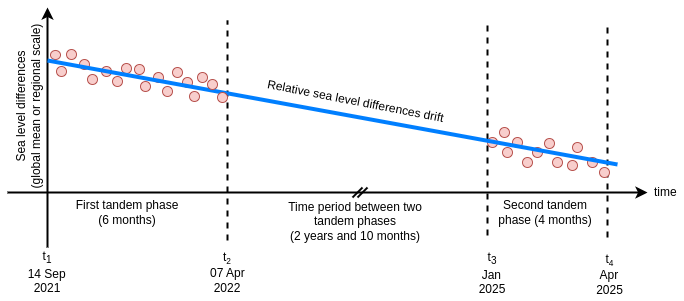
Figure 1 Basic principle of the two-tandem-phase method applied to the Jason-3 and S6-MF altimetry satellites.

In this paper, we demonstrate the ability of the two-tandem-phase method to assess instrumental stability. We explain the method developed to quantify the uncertainty in the two-tandem-phase method in Sect. 2. We assess the global uncertainty in the two-tandem-phase method, which varies depending on the length of the second tandem phase and the interval between the two phases in Sect. 3. Additionally, we evaluate the method's uncertainty at regional scales by examining its sensitivity to spatial scales ranging from several hundred to a thousand kilometers. Finally, we compare the uncertainty obtained with other validation methods to highlight the benefits of the second tandem phase for assessing the instrumental stability in Sect. 4. We also discussed the results with regard to the scenario foreseen for the second tandem phase between Jason-3 and S6-MF (Ferrier, 2023) planned for early 2025 for a duration of 4 months, i.e., 2 years and 9 months after the end of the first tandem phase.

2 Methodology for estimating uncertainty in the two-tandem-phase method

This section presents the methodology developed in this study to estimate the uncertainty associated with the two-tandem-phase method. The uncertainty in the two-tandem-phase method is characterized by the uncertainty in sea level trends over the duration of both tandem phases (depicted by the blue line in Fig. 1). Our method is based on the framework established by Ablain et al. (2019) and Prandi et al. (2021), which evaluates uncertainties in trends at both global and regional scales.

2.1 Uncertainty budget assessment during a tandem phase

Initially, the methodology involves establishing an uncertainty budget for sea level differences within a tandem phase. The uncertainty budget for the global mean sea level (GMSL), as described in Ablain et al. (2019), pinpoints various error sources in altimetry data, such as environmental corrections, precise orbit determination (POD), instrumental noise, and instrumental drift and offset, which contribute to the uncertainties in the GMSL series. The uncertainty budget also provides the statistical properties of these errors, including the temporal correlation and standard deviation for each error source. During a tandem phase, the uncertainty budget for sea level differences is significantly simplified since most uncertainties included in the mean sea level uncertainty budget are canceled out (e.g., geophysical and atmospheric corrections, long-term time-correlated effects in POD). It only covers uncertainties arising from short-term time-correlated effects previously stated in Sect. 1, which result from sea level differences in altimeter measurements, the POD, and the mean sea surface between two altimeter missions.

2.1.1 Mean sea level difference calculations during the tandem phase

We calculate the sea level estimates over the three tandem phases between Jason-1 and Jason-2 (August 2008–January 2009), between Jason-2 and Jason-3 (February 2016–October 2016), and between Jason-3 and S6-MF (September 2021–April 2022). It should be mentioned that the tandem phase between Jason-3 and S6-MF started on 17 December 2020 and ended on 4 April 2022. However, an instrumental anomaly was detected on side A of the S6-MF altimeter (Poseidon-4) a few months after the launch of S6-MF. Thus, on 14 September 2021 a switch was operated on side B of the S6-MF altimeter (Dinardo et al., 2022). Therefore, the data of the first tandem phase between S6-MF and Jason-3 can be used after the side B change from 14 September 2021 to 4 April 2022. For Jason-1, Jason-2, and Jason-3, the altimeter products used are the non-time-critical (NTC) along-track level-2+ (L2P) products from the Copernicus Marine Service under CNES responsibility. These products are downloaded from the AVISO FTP website (http://ftp-access.aviso.altimetry.fr/uncross-calibrated/open-ocean/non-time-critical/l2p/sla/, last access: 15 January 2025) and contain the along-track sea level anomaly data at 1 Hz (SLA; see Eq. 1) calculated after applying a validation process that is fully described in the product handbook of each altimetry mission (Along-track Level-2+ (L2P) Sea Level Anomaly Sentinel-3/Jason-CS-Sentinel-6 Product Handbook, 2022). We use version 03_00, which is the current product version of Sentinel-3 and S6-MF L2P, with reprocessing from Baseline Collection 004 (PB2.61) and Baseline Collection F05, respectively. The along-track SLA provided in the L2P products is derived from the following equation:

$$\begin{array}{}\text{(1)}& \begin{array}{rl}\mathrm{SLA}& =\text{Orbit}-\text{Range}-{\mathrm{\Sigma }}_i{\text{Correction}}_i\\ & -\text{Mean}\text{Sea}\text{Surface},\end{array}\end{array}$$

where “Orbit” is the radial distance between the satellites and the geoid, “Range” the distance between the satellite and the sea surface, Σ_iCorrection_i is the sum of the geophysical and atmospheric corrections to be applied (e.g., ocean, polar and earth tides, wet and dry troposphere corrections, sea state bias correction), and “Mean Sea Surface” is the mean of the sea surface height from which sea level anomalies are derived. The geophysical corrections applied in L2P products for the SLA calculation are already homogenized for each altimetry mission and identical during a tandem phase. We have also verified that the sea level estimates remain consistent during a tandem phase regardless of whether geophysical and atmospheric corrections are applied. It should also be noted that the wet troposphere correction derived from microwave radiometers has not been applied to the sea level calculation to avoid the introduction of instrumental errors not related to the altimeter measurements.

We have calculated the GMSL differences between two altimeter missions during a tandem phase applying the GMSL AVISO method described in Henry et al. (2014). In summary, the along-track 1 Hz SLA measurements have first been averaged within grid cells for each orbital cycle (≈9.91 d for reference altimetry missions). We have made this computation for each altimeter mission separately. As recommended by Henry et al. (2014), cells of 1° latitude by 3° longitude have been applied to optimize the effect of sea level variability observed by reference altimeter missions in the GMSL. We then calculated the SLA differences at regional scales for each cycle of the tandem phase, directly calculating the differences between the SLA grids of each altimeter mission. The time series of GMSL differences has then been obtained after spatially averaging the grids of SLA differences at each cycle with a weighting that accounts for the relative ocean area covered.

2.1.2 Uncertainty budget on the global scale

To characterize uncertainties arising from short-term time-correlated effects, we analyzed GMSL differences during tandem phases of Jason-1 and Jason-2, Jason-2 and Jason-3, and Jason-3 and Sentinel-6 Michael Freilich (S6-MF) (over the side B period). This involved calculating the standard deviation and time correlation of the GMSL differences. We plotted these differences in the middle panel of Fig. 2. During the Jason-3 and S6-MF tandem phase, the GMSL differences exhibit a 2-month periodic signal. Cadier et al. (2024) recently identified that this signal arises from beta-prime dependencies in the Centre National d'Études Spatiales (CNES) POD solution used for S6-MF. Furthermore, Cadier et al. (2024) demonstrated that using Jet Propulsion Laboratory (JPL) POD solutions substantially reduces this signal. Assuming that the identified beta-prime dependencies will be fully corrected in the updated S6-MF CNES POD, we removed this 2-month periodic signal before calculating the standard deviation of the GMSL differences. This reduced the standard deviation from 0.99 to 0.48 mm, providing a more realistic value. The GMSL differences before removing this periodic signal are shown by the dashed line in Fig. 2f. The standard deviations derived from the three tandem phases are within 0.07 mm for Jason-2 and Jason-3 (0.41 mm) and Jason-3 and S6-MF (0.48 mm). However, the standard deviation is slightly higher for Jason-1 and Jason-2 (0.69 mm), most likely due to additional errors in the precise orbit calculation of Jason-1.

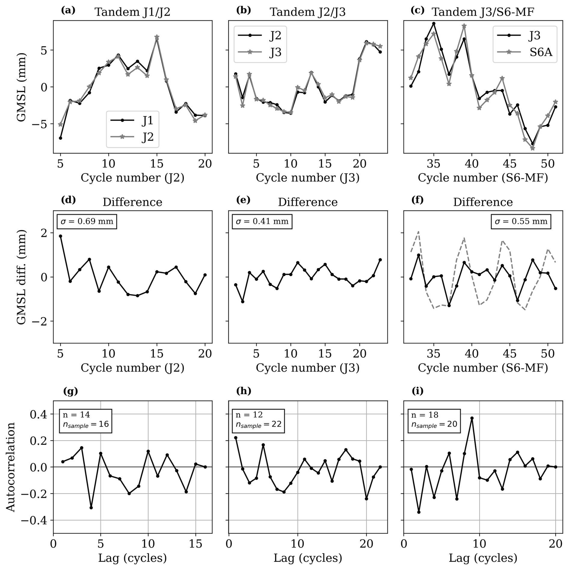
Figure 2 Panels (a)–(c) show GMSL records over the tandem phase between (a) Jason-1 and Jason-2 (J1/J2), between (b) Jason-2 and Jason-3 (J2/J3), and between (c) Jason-3 and S6-MF (side B) on the right (J3/S6-MF). Panels (d)–(f) show the GMSL record differences between the two respective missions in tandem phase. Here, σ is the standard deviation of the GMSL differences. The dashed grey line in panel (f) is the GMSL differences before removal of the 60 d periodic signal. Panels (g)–(i) show the autocorrelation of the difference signal, where n is the number of independent measurements of the sample and n_sample the total number of measurements of the sample. The mean value of each time series has been removed to facilitate comparison.

The autocorrelation of each GMSL difference, shown in the bottom row of Fig. 2, does not exhibit a significant autocorrelation at any lag. The number of independent measurements (n) of GMSL differences, displayed in the legend of Fig. 2 (bottom panel), was calculated following the methodology of Guérou et al. (2023). This method uses the following equation:

$$\begin{array}{}\text{(2)}& n={\displaystyle \frac{(\mathrm{1}-{\mathit{\rho }}_{\mathrm{1}})}{(\mathrm{1}+{\mathit{\rho }}_{\mathrm{1}})}}\cdot n_{\text{sample}},\end{array}$$

where ρ₁ is the first-lag autocorrelation coefficient, representing the correlation between consecutive measurements, and n_sample is the total number of measurements of the sample. For all three tandem phases, the number of independent measurements is high. For S6-MF and Jason-3, n=18 (for a total of n_sample=20), implying that GMSL differences largely decorrelate after approximately three measurements or 30 d (one measurement per cycle). On the basis of these analyses, we assume that the GMSL differences are fully decorrelated beyond 1 month during these three analyzed tandem phases. Therefore, the uncertainty budget of the GMSL differences during a tandem phase was established by incorporating a single 1-month time-correlated error with a standard deviation of 0.5 mm (see Table 1). Each tandem phase yields similar but not identical results. This can be attributed to differences in the GMSL between the altimetry missions and the relatively short duration (approximately 6 to 9 months) of the tandem phases. To assess the sensitivity of our results to these factors, a sensitivity analysis was conducted (see Sect. 3) by varying the temporal correlation from 0 to 2 months and the standard deviation of the GMSL differences from 0.4 to 0.6 mm.

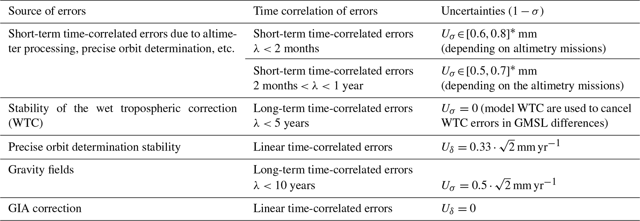
Table 1 Uncertainty budget of GMSL differences between two altimetry missions in tandem.

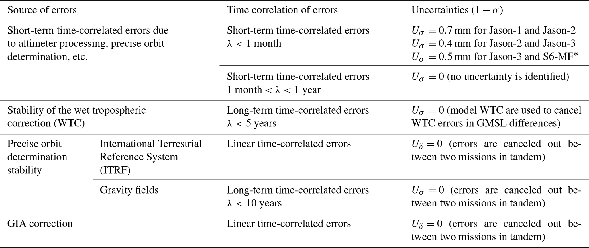
^* The uncertainty budget in this study is constructed by taking the U_σ for Jason-3 and S6-MF.

2.1.3 Uncertainty budget at regional scales

The uncertainty budget for sea level differences, established on a global scale in Sect. 2.1.2, can be adapted to regional scales ranging from a few hundred to a few thousand kilometers. This regional adaptation is based on the framework presented by Prandi et al. (2021) for regional sea level uncertainty. Most of the different sources of uncertainties outlined in Prandi et al. (2021) cancel out on the global scale when considering sea level differences during a satellite altimeter tandem phase. Therefore, the uncertainty budget of regional sea level differences during a tandem phase only contains uncertainties due to short-term time-correlated errors. To quantify this uncertainty, regional sea level differences between Jason-3 and S6-MF were computed during their tandem phase. Differences were calculated for varying cell sizes, from 3°×3° to 36°×36° (corresponding to approximately 300 km × 300 km and 4000 km × 4000 km, respectively). The standard deviation of these differences was then calculated within each cell size. This standard deviation, representing the uncertainty due to the 1-month correlated errors, was incorporated into the regional uncertainty budget (see Table 2) homogeneously to the uncertainty budget at a global scale.

Table 2 Uncertainty budget of regional sea level differences between two altimetry missions in tandem. Values are provided for cell sizes ranging from 3°×3° to 36°×36°. They are dependent on the location, and here we provide the median value.

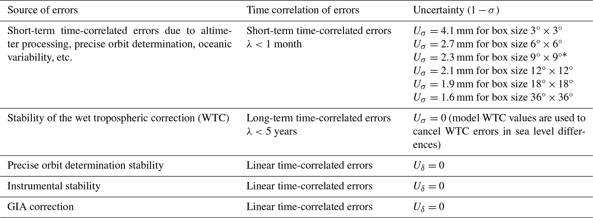
^* The uncertainty budget in this study is constructed by taking the U_σ for a box size of 9°×9°.

2.2 Error covariance matrix

After specifying the uncertainty budget, the error covariance matrix for sea level differences observed during a tandem phase (Σ_tp, where tp stands for tandem phase) is derived using the methodology outlined in Ablain et al. (2019). The uncertainty budget contains only one source of uncertainty with short-term time-correlated errors. The covariance matrix has been modeled applying a Gaussian attenuation function determined by the wavelength of the time-correlated errors, expressed as $e^{-\frac{\mathrm{1}}{\mathrm{2}}{\left(\frac{t}{\mathit{\lambda }}\right)}^{\mathrm{2}}}$, where the correlation timescale λ is set to 1 month (see Sect. 2.1.2). The resulting covariance matrix has a diagonal structure with smaller off-diagonal terms.

The error covariance matrix of the relative errors observed during the two tandem phases, Σ, is partitioned into two distinct diagonal blocks: the error covariance matrix for the first tandem phase (Σ_{tp_1}) and the second tandem phase (Σ_{tp_2}), as shown below.

$$\begin{array}{}\text{(3)}& \textcolor{red}{}\end{array}$$

Since the second tandem phase has not yet been executed, we assume the same error characteristics (standard deviation and temporal correlation) as those of the first tandem phase. Both tandem phases involve the same altimeter systems (e.g., Jason-3 and S6-MF), and factors such as instrumental noise, POD, and mean sea surface are expected to remain consistent across both phases. Therefore, the error characteristics can reasonably be assumed to be similar.

2.3 Mathematical formalism to derive uncertainty in trends

Finally, we use this error covariance matrix (Σ) to calculate the uncertainty in the trend of sea level differences. The formalism used is also based on Ablain et al. (2019). The trend is fitted from a linear regression model ($\mathit{y}=\mathit{X}\mathit{\beta }+\mathit{ϵ}$) applying an ordinary least-squares (OLS) approach where the estimator of β with the OLS, denoted as $\widehat{\mathit{\beta }}$, is determined as follows:

$$\begin{array}{}\text{(4)}& \widehat{\mathit{\beta }}\sim ({\mathit{X}}^t\mathit{X}{)}^{-\mathrm{1}}{\mathit{X}}^t\mathit{y},\end{array}$$

where X is the time vector that contains the date of each altimeter cycle during the two tandem phases, while y is the observation vector that contains the sea level differences averaged over each complete cycle. The uncertainty in the trend is given by $\widehat{\mathit{\beta }}$, which is the distribution of the estimator following a normal law:

$$\begin{array}{}\text{(5)}& \widehat{\mathit{\beta }}=N(\mathit{\beta },({\mathit{X}}^t\mathit{X}{)}^{-\mathrm{1}}\left({\mathit{X}}^t\mathbf{\Sigma }\mathit{X}\right)\left({\mathit{X}}^t\mathit{X}{)}^{-\mathrm{1}}\right).\end{array}$$

It should be noted that the calculation of trend uncertainty does not depend on sea level differences (y) but only on the time vector (X) and the error covariance matrix (Σ). This allows us to analyze the uncertainty in the two-tandem-phase method even though the second tandem phase has not yet been performed. This study is based on the assumption that the uncertainty budget of the second tandem phase will be the same as that of the first.

3 Uncertainty in the two-tandem-phase method

3.1 On the global scale

The uncertainty in the trend of sea level differences in the two-tandem-phase method is calculated on the global scale with the uncertainty budget described in Table 1. The uncertainty budget in this study is constructed by taking the U_σ for Jason-3 and S6-MF. The duration of the first tandem phase is set at 6 months, corresponding to the duration of the tandem phase between Jason-3 and the altimeter side B of S6-MF (14 September 2021 to 7 April 2022). For the second tandem phase, we analyze the impact on the trend uncertainty in both the duration of the second tandem phase and the time elapsed since the first tandem phase. To construct the error covariance matrix (Σ; see Eq. 3), we use the same uncertainty budget for both tandem phases (see Table 1). Figure 3 shows the evolution of the uncertainty in the trend of GMSL differences as a function of the time period between the two tandem phases (between 1 and 6 years) for four different time spans of the second tandem phase (from 1 to 6 months). For a 1-year time span between the two tandem phases, the uncertainties range from 0.27 mm yr⁻¹ for a second-phase duration of 6 months to 0.41 mm yr⁻¹ for a second-phase duration of 1 month. They are reduced to about 0.12–0.16 mm yr⁻¹ after 3 years between the two tandem phases. They are less than 0.10 mm yr⁻¹ after 5 years between the two tandem phases with an interval of 0.02 mm yr⁻¹. These results show that the uncertainty in the trend of the GMSL differences is less influenced by the duration of the second tandem phase when the time elapsed between the two tandem phases increases. For instance, for a time span of 2 years, the uncertainties in the trend range from 0.24 to 0.16 mm yr⁻¹ for a second tandem phase of 1 month and 6 months, respectively. For a time span of 5 years, the uncertainties in the trend range from 0.10 to 0.08 mm yr⁻¹. On the basis of these results, it is recommended that the second tandem phase be carried out as far as possible from the first (at least a few years later), but it is not necessary for this second phase to be very long. A period of 4 months is considered sufficient to verify the instrumental stability on the global scale.

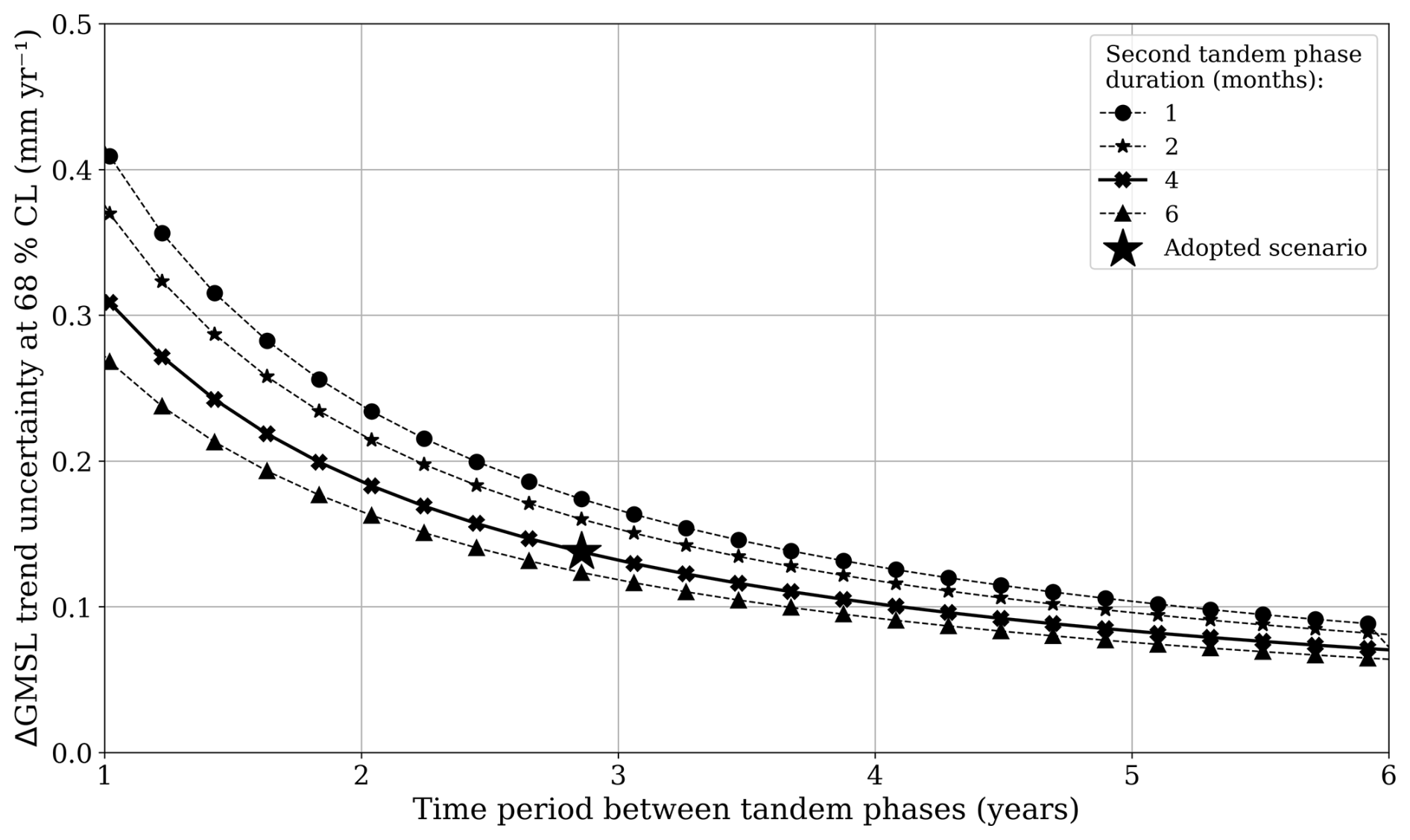
Figure 3 Evolution of the uncertainty in the trend of GMSL differences (ΔGMSL) with the time elapsed between the two tandem phases between Jason-3 and S6-MF for several durations of the second tandem phase that range from 1 to 6 months. The scenario adopted by the space agencies for the second tandem phase, which is 4 months long and separated by 2 years and 9 months from the first phase, is indicated with a star.

It should be noted that similar analyses carried out before the launch of S6-MF led to the same recommendation (Ablain et al., 2020). This helped space agencies specify a scenario for the second tandem phase between Jason-3 and S6-MF. The second tandem phase should start in January 2025, which is 2 years and 9 months after the first tandem phase, and run for a duration of 4 months (Ferrier, 2023). This adopted scenario is shown with a star in Fig. 3. It leads to an uncertainty in the trend of GMSL differences of 0.14 mm yr⁻¹.

The results we obtained are contingent upon how the uncertainty budget of sea level differences is specified during a tandem phase (see Table 1). As previously stated, the uncertainty budget may be subject to minor modifications depending on the length of the tandem phase and the altimeter missions involved. Thus, we performed a sensitivity analysis by varying the temporal correlation from 0 to 2 months and varying the standard deviation of GMSL differences between 0.4 and 0.6 mm within the uncertainty budget. The uncertainties in the trend range from 0.06 to 0.18 mm yr⁻¹ when only the temporal correlation is altered and from 0.11 to 0.17 mm yr⁻¹ when only the variance is varied in the case of the scenario adopted between S6-MF and Jason-3 for the second tandem phase. In the worst case, corresponding to a temporal correlation of 2 months and a variance of 0.6 mm, the maximum uncertainty in the trend is 0.21 mm yr⁻¹. This sensitivity analysis in the uncertainty budget indicates a low sensitivity in the absolute value of the trend uncertainty (±0.07 mm yr⁻¹).

3.2 At regional scales

The uncertainty in the trend of sea level differences in the two-tandem-phase method is calculated at regional scales with the uncertainty budget described in Table 2. The duration of the first tandem phase remains fixed to 6 months. We also fixed the duration of the second tandem phase to 4 months. We also use the same uncertainty budget for both tandem phases specified at regional scales (see Table 2) to construct the error covariance matrix (Σ; see Eq. 3). Different spatial scales are analyzed with cell sizes ranging from 3° × 3° (330 km × 330 km) to 36° × 36° (4000 km × 4000 km). Figure 4 shows the evolution of the uncertainties in the trend of regional mean sea level differences for these different configurations as a function of the time elapsed between the two tandem phases. Uncertainties decrease with increasing cell size. After 2 years and 9 months, corresponding to the scenario adopted for the second tandem phase between S6-MF and Jason-3, the uncertainty ranges from 1.1 mm for a size box of 3° × 3° (330 km × 330 km) to 0.4 mm for a size box 36° × 36° (4000 km × 4000 km). Detecting trends in regional mean sea level differences lower than 1 mm yr⁻¹ is possible in almost all ocean basins using a second tandem phase as early as 2 years after the first phase.

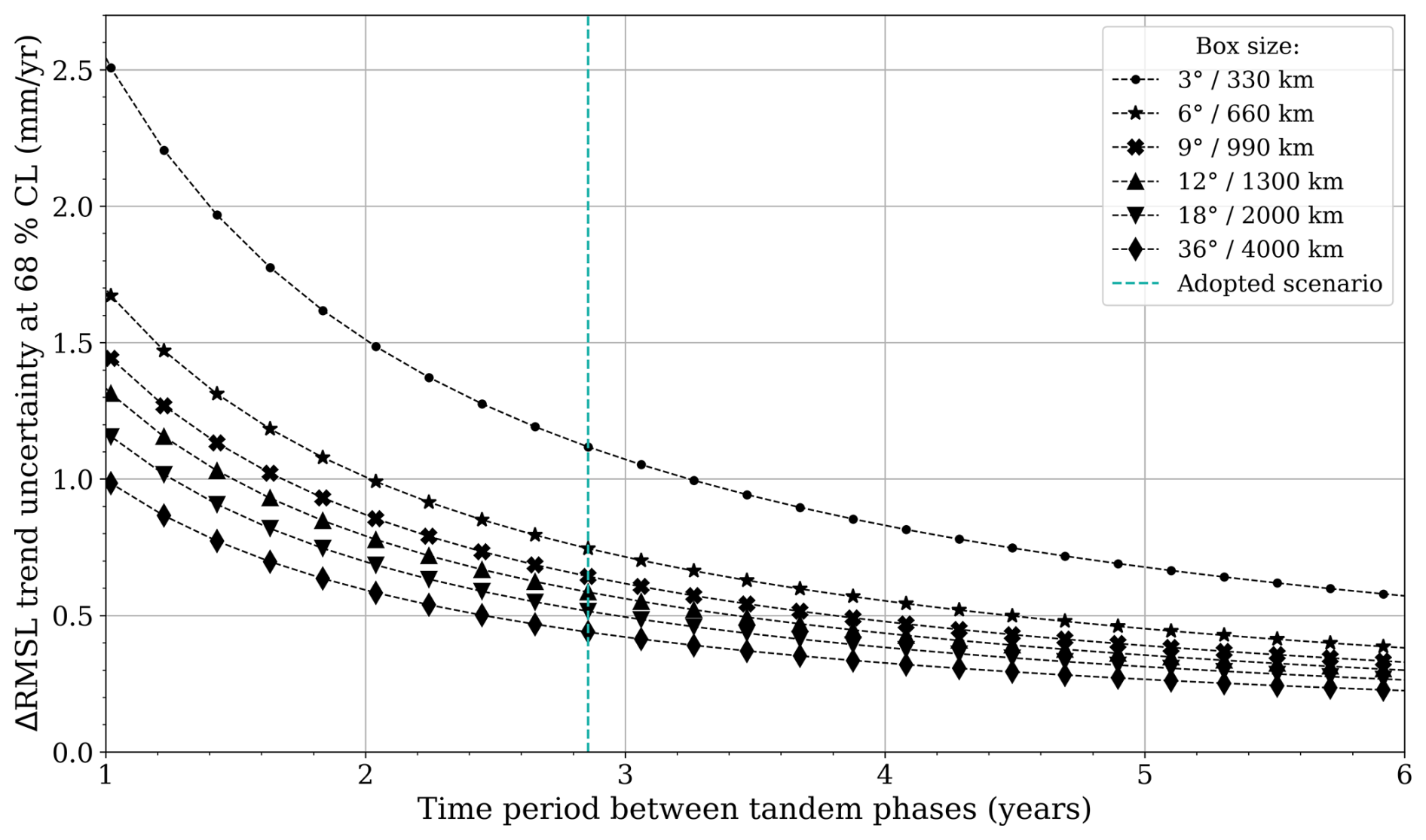
Figure 4 Evolution of the uncertainty in the trend of regional mean sea level differences (ΔRMSL) with the time period between the two tandem phases between Jason-3 and S6-MF for different cell sizes from 3° × 3° (corresponding to ∼330 km spatial scale) to 36° × 36° (corresponding to ∼4000 km spatial scales).

4 Comparison with other validation methods

4.1 Uncertainty budgets of other validation methods

To assess the uncertainty in the two-tandem-phase method, we compare it with the following two established approaches: (a) sea level comparisons between two altimetry missions on different orbits (hereafter referred to as the without-tandem-phase method) (Jugier et al., 2022) and (b) sea level comparisons between altimeter and tide gauge data (Valladeau et al., 2012; Watson et al., 2015). These methods were selected because their ability to detect drift in GMSL has previously been demonstrated using uncertainty budgets similar to the approach employed in this study (see Sect. 2). For the without-tandem-phase method, the uncertainty budget developed by Jugier et al. (2022) was used. This budget, presented in Table A1 for the global scale and Table B1 for regional scales, accounts for the spatial and temporal differences (typically a few days and a few dozen kilometers, respectively) inherent in altimetry measurements from altimeter missions over different orbits. These differences introduce uncertainties related to geophysical and atmospheric effects, oceanic variability, and long-period time-correlated errors in the POD. Similarly, the uncertainty budget for altimeter–tide gauge comparisons, presented in Ablain et al. (2018) accounts for spatial and temporal differences between tide gauges and altimetry measurements (typically a few hours and a few dozen kilometers, respectively). Furthermore, all of the errors created by the two independent system measurements are not canceled out by the sea level differences. The uncertainty budget, presented in Table C1 for the global scale, includes uncertainties associated with geophysical and atmospheric effects, oceanic variability, and long-period time-correlated errors in both altimetry (e.g., POD) and tide gauge records (e.g., land motion correction). This limitation arises primarily from uncertainties in tide gauge records, including vertical land motion due to tectonic activity and subsidence, and the spatial offset between tide gauges and altimetry measurements (Valladeau et al., 2012; Watson et al., 2021). However, highly accurate local comparisons are possible in regions with well-referenced tide gauges, such as those described by Mertikas et al. (2021).

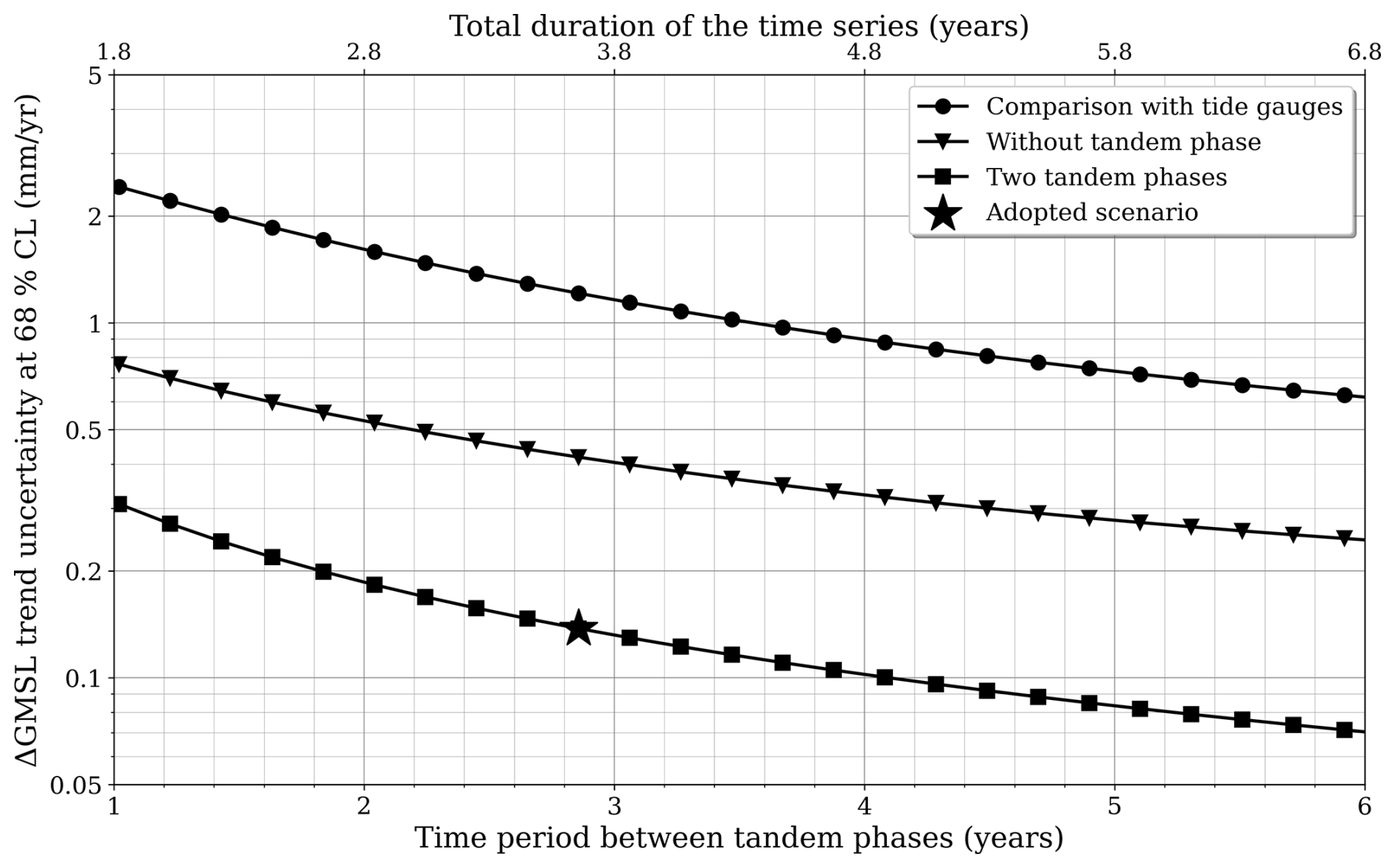
Figure 5 Evolution of the uncertainty in the trend of GMSL differences (ΔGMSL) with the time spent between the two tandem phases of Jason-3 and S6-MF for the different calibration methods: (a) comparison with tide gauges, (b) inter-mission comparison without a tandem phase, (c) and inter-mission comparison with two tandem phases. The scenario adopted for the second tandem phase, which is 4 months long and separated from the first phase by 2 years, is indicated with a star. The scale of the y axis is logarithmic.

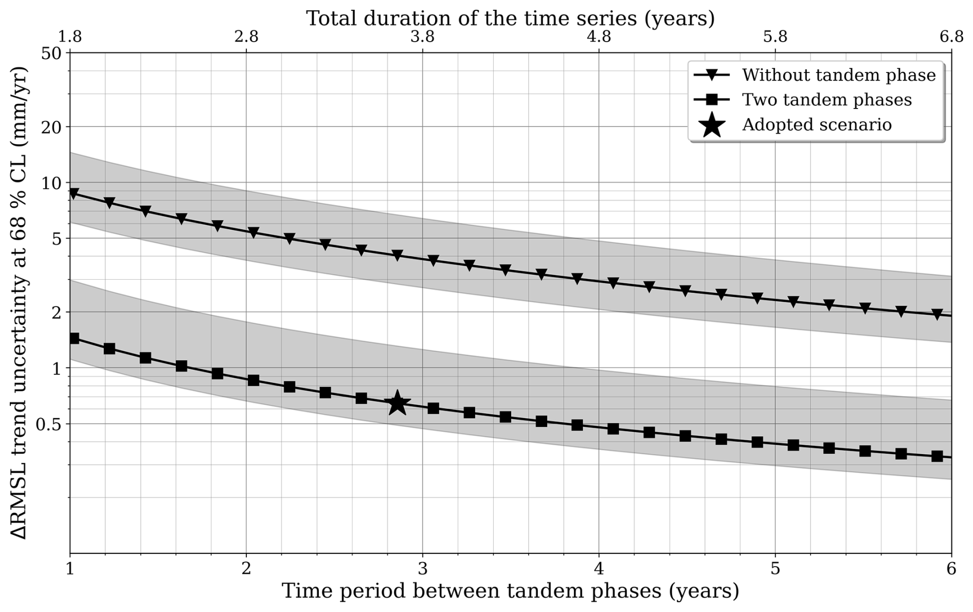
Figure 6 Evolution of the trend uncertainty in regional mean sea level differences (ΔRMSL) with the time period between the two tandem phases between Jason-3 and S6-MF for different calibration methods and a cell size of 9° × 9° (corresponding to ∼1000 km spatial scale). The envelope represents the spatial distribution of uncertainties between the 16th and 84th percentile (i.e., 1−σ) values. The scale of the y axis is logarithmic. The scenario adopted for the second tandem phase, which is 4 months long and separated by 2 years and 9 months from the first phase, is indicated with a star.

4.2 On the global scale

In Fig. 5, the uncertainties have been plotted for the three validation methods (two-tandem-phase, without-tandem phase, altimeter–tide gauge comparisons) as a function of the time spent between the two tandem phases of Jason-3 and S6-MF. The duration of the second tandem phase has been set at 4 months according to the adopted scenario Ferrier (2023). It is also worth noting that the total duration of the time series used to calculate the uncertainties for all methods includes the duration of both tandem phases. This means that for 1 year spent between the two tandem phases, the total length of the time series is 1 year and 10 months (1 year + 6 months + 4 months). Similarly, for the adopted scenario of a second tandem phase of 4 months that takes place 2 years and 9 months after the first phase that took 6 months, the total duration of the analyzed time series is 3 years and 7 months. The analysis in Fig. 5 clearly shows that the two-tandem-phase method significantly reduces the uncertainties in the trend of the GMSL differences. Over a period of 3 years and 7 months, which corresponds to the adopted scenario, the uncertainty is 1.2 mm yr⁻¹ with the tide gauge method. It is reduced to 0.42 mm yr⁻¹ for the without-tandem-phase method, whereas the uncertainty decreases to 0.14 mm yr⁻¹with the new two-tandem-phase method. Increasing the time spent between the two Jason-3 and S6-MF tandem phases to 4 years, and hence the total duration to 4 years and 10 months, leads to lower uncertainties for the tide gauge, without-tandem-phase, and two-tandem-phase method of 0.9, 0.35, and 0.1 mm yr⁻¹, respectively. These results highlight the better ability of the two-tandem-phase method to assess instrumental stability on the global scale.

4.3 At regional scales

Similarly to the global scale, we compare the two-tandem-phase method with the method based on sea level comparisons between two altimetry missions on different orbits (outside a tandem phase). In Fig. 6 we evaluate the evolution of the uncertainty in the trend of the regional mean sea level differences in the two methods with the time elapsed between two tandem phases, after selecting size boxes of 9° × 9° (about 1000 km). As uncertainties are not spatially homogeneous (see Fig. A1), we have also plotted the envelope of the spatial distribution of uncertainties at values between the 16th and 84th percentile (i.e., 1−σ) in Fig. 6. For a cell size of 9° by 9° (about 1000 km by 1000 km), the uncertainty at 1−σ ranges from 1.8 to 4.8 mm with a median of 2.3 mm. We observe that the average value of trend uncertainty is even more significantly reduced at regional scales than on the global scale with the two-tandem-phase method. By conducting the analysis over 3 years and 7 months, corresponding to the adopted scenario of a second tandem phase 2 years and 9 months after the initial phase, the trend uncertainty in sea level differences is 4.0 mm yr⁻¹ in without-tandem-phase method, while with the new two-tandem-phase method the uncertainty decreases to 0.65 mm yr⁻¹. Increasing the total duration of the analysis to 4 years and 10 months (corresponding to 4 years between the two tandem phases of Jason-3 and S6-MF) results in lower uncertainties for each validation method of 3.0 and 0.5 mm yr⁻¹, respectively. Significantly better results obtained at regional scales are mainly explained as being due to ocean variability. As mentioned above, it is a significant source of uncertainty when measurements are not colocated in time and space. At regional scales, the effect of ocean variability is not spatially averaged and becomes a major source of uncertainty. As the two-tandem-phase method is not affected by this, its ability to assess instrumental stability on regional scales is very promising.

5 Conclusions

We have proposed a novel cross-validation method to assess the instrumental stability of the altimetry satellite based on the realization of a second tandem phase between two successive reference missions a few years after the initial phase. We have demonstrated the ability of the two-tandem-phase method to assess the instrumental stability. Assuming a second tandem phase with a minimal duration of 4 months, it will be possible to assess instrumental stability on the global scale with an uncertainty of less than ±0.1 mm yr⁻¹ in a CL of [16 %–84 %] for time periods of 4 years and beyond between the two tandem phases. This means 3 and 8 times better accuracy than when using other validation methods based on sea level comparisons outside a tandem phase and based on altimetry and tide gauge comparisons, respectively,. On regional scales, the gain is greater, with an uncertainty of ±0.5 mm yr⁻¹ in a CL of [16 %–84 %] for spatial scales of about 1000 km, which is 6 times better than that found with the method based on sea level comparisons outside a tandem phase. The two-tandem-phase method could be applied for the first time between S6-MF and Jason-3 after the realization of the second tandem phase in early 2025. It will be possible to assess sea level stability with an uncertainty of ±0.14 mm yr⁻¹ in a CL of [16 %–84 %] on the global scale for the scenario adopted for the second tandem phase between Jason-3 and S6-MF. On regional scales, it will be possible to assess sea level stability with an uncertainty of ±0.65 mm yr⁻¹ in a CL of [16 %–84 %] for spatial scales of about 1000 km. To date, we have assumed that the uncertainty budget of relative errors will be the same over the two tandem phases between S6-MF and Jason-3. This should be re-evaluated after the completion of the second tandem phase, and the uncertainties in the trend may be updated as a result. If a significant instrumental drift in sea level is detected, it cannot automatically be attributed to the S6-MF or Jason-3 altimetry missions. In-depth investigations will have to be carried out by experts from the two satellites, and alternative validation methods will also have to be implemented, even if they are less accurate in detecting a drift in altimeter measurements. These inquiries could lead to revisions in the mean sea level uncertainty budget to reflect uncertainties in the instrumental stability.

The performance of the two-tandem-phase method is very promising. However, the novel method also presents some limitations. The method is only applicable over the period encompassing the two tandem phases and does not allow the assessment of the altimeter stability outside this period. This method only allows for the assessment of the stability of instrumental errors since all the other sources of error have been canceled out (e.g., geophysical and atmospherical effects, long-term errors in the POD). Therefore, no assessment of other sources of error is made in the uncertainty budget of the mean sea level (Ablain et al., 2019; Guérou et al., 2023; Prandi et al., 2021). For these reasons, the other validation methods are complementary, although their uncertainties in the trend of sea level differences are higher.

In order to reap a larger benefit from this novel cross-validation method, we need to regularly implement double tandem phases between two successive altimetry missions in the future. The instrumental stability could be assessed over a long period. Assuming that it is theoretically possible to organize a third tandem phase between Jason-3 and S6-MF 6 years after the initial tandem phase, we could assess instrumental stability with uncertainties of ±0.07 mm yr⁻¹ ([16 %–84 %] CL) on the global scale (see Fig. 5) and approximately ±0.3 mm yr⁻¹ ([16 %–84 %] CL) at regional scales (see Fig. 4). The feasibility of conducting regular tandem phases between reference missions needs to be analyzed while taking the end-of-life limitations of the reference missions into consideration.

Appendix A

Table A1 Uncertainty budget of the GMSL differences between two altimetry missions that are not in tandem (from Jugier et al., 2022).

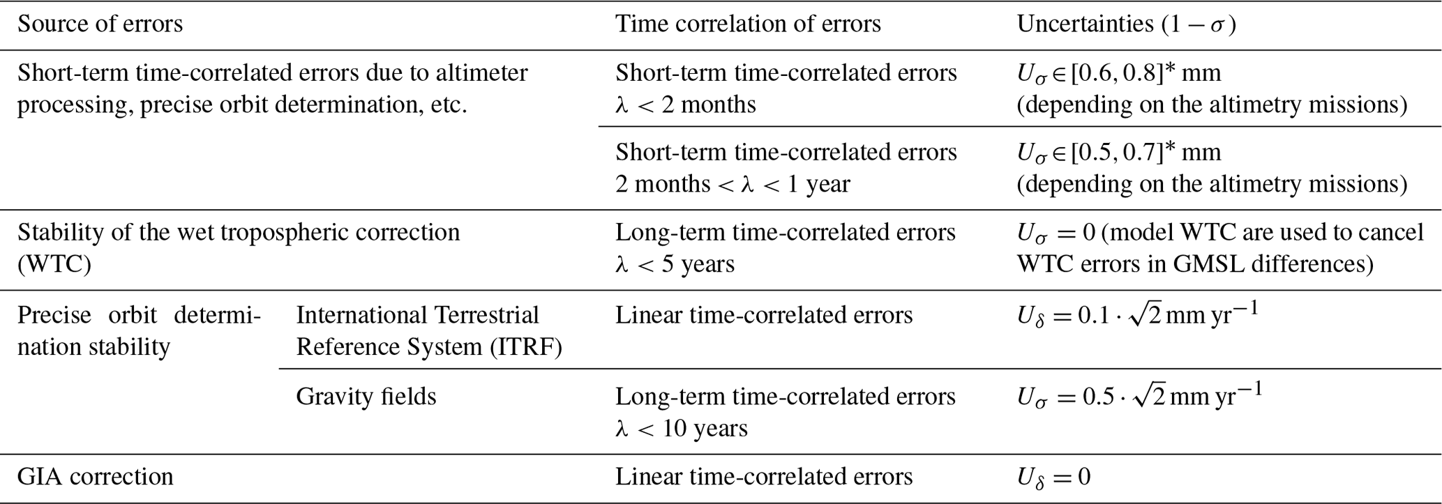
^* The uncertainty budget in this study is constructed by taking the mean value of the range, which is U_σ=0.7 mm for λ<2 months and U_σ=0.6 mm for 2 months $<\mathit{\lambda }<\mathrm{1}$ year.

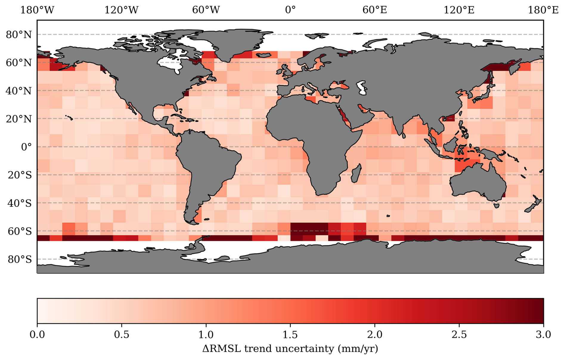
Figure A1 Uncertainties in the trend of regional mean sea level differences in the two-tandem-phase method for a 9°×9° cell size and for a time difference of 2 years and 9 months between the two Jason-3 and S6-MF tandem phases.

Appendix B

Table B1 Uncertainty budget of the regional mean sea level differences between two altimetry missions that are not in tandem (from Jugier et al., 2022). Values are provided for 9°×9° box sizes within a 16th-percentile and 84th-percentile interval.

^* The uncertainty budget in this study is constructed by taking the median value, which is U_σ=9.4 mm for λ<2 months and U_σ=4.9 mm for 2 months $<\mathit{\lambda }<\mathrm{1}$ year.

Appendix C

Table C1 Uncertainty budget of GMSL differences between altimeter measurements and tide gauges data from the GLOSS and CLIVAR network (from Ablain et al., 2018).

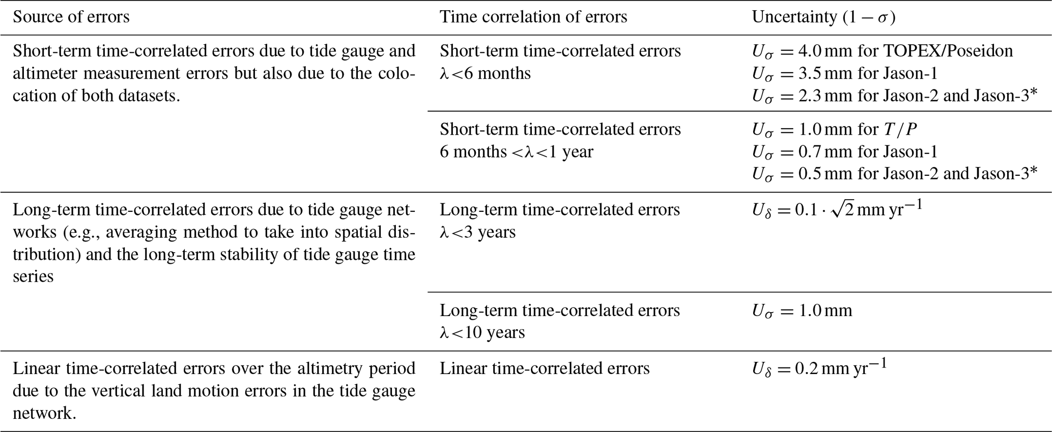
^* The uncertainty budget in this study is constructed by taking the U_σ for Jason-2 and Jason-3.