Internal tides off the Amazon shelf in the western tropical Atlantic: analysis of SWOT Cal/Val mission data

This study focuses on the internal tides (ITs) off the Amazon shelf in the tropical Atlantic. It is based on 2 km horizontally gridded observations along the swaths of SWOT (Surface Water and Ocean Topography) track 20 during the calibration/validation phase (Cal/Val, 1 d orbit) from late March to early July 2023. We evaluate the amplitude of M2, N2, and S2 frequencies and use the M2 atlas as an internal tide correction model for SWOT observations. Internal tide amplitudes (models or atlases) are first derived by harmonic analysis of the SWOT sea level anomaly (SLA). The estimation is improved by performing a principal component analysis before the harmonic analysis. The results compare very well with the high-resolution empirical tide (HRET) internal tide model, the reference product for internal tide corrections in altimetry observations. The coherent mode 1 and mode 2 M2 can be distinguished in the internal tide model derived from SWOT, while the higher modes with their strong SLA signature are seen mostly in the incoherent part. In comparison to HRET, the correction of SWOT observations with SWOT-based atlases may be more relevant for this track.

1 Introduction

The launch of the SWOT (Surface Water and Ocean Topography) mission at the end of 2022 certainly marks a new phase in spatial altimetry. SWOT is equipped with the KaRIn instrument, a Ka-band radar interferometer capable of measuring the sea surface topography with unprecedented resolution in two-dimensional swaths. KaRIn consists of two antennae that take 2D measurements in two 50 km wide swaths separated by a 20 km gap covered by the conventional nadir radar altimeter also carried by the mission. The accuracy of SWOT's instruments is such that SWOT should be able to observe the ocean down to a spatial scale of 15–30 km (Morrow et al., 2019; Dufau et al., 2016; Wang and Fu, 2019), thus complementing our 2D view of the ocean with TOPEX/Poseidon-class nadir altimetry, which is limited to scales larger than 150 km (Chelton et al., 2011; Ballarotta et al., 2019) along one-dimensional tracks rather than two-dimensional swaths. The main oceanographic objective of the SWOT mission is to characterize mesoscale and sub-mesoscale ocean circulation (Fu et al., 2012; Fu and Ubelmann, 2014). However, ocean processes at the scales targeted by SWOT (150–15 km) encompass both “balanced” geostrophic and “unbalanced” ageostrophic motions, including surface and internal inertia-gravity waves at tidal frequencies. The correction of internal tide (IT) surface signatures presents a significant challenge to the useability of SWOT data, considering that the spatial scales of these waves overlap with those of balanced motions. Conversely, the exploitation of SWOT data to study ITs is an opportunity for learning more about these waves and quantifying their impacts in the ocean.

Efforts have been made in recent years to map internal tides using conventional altimetry observations. This was made possible by the fact that the internal tide has a SSH (sea surface height) signature of the order of 1 cm to several centimetres (Ray and Mitchum, 1997). However, the coarse sampling in both space and time of conventional altimetry is a hindrance. To derive spatially continuous high-resolution maps of the internal tide SSH from the sparse altimeter sampling, Dushaw (2015), Zhao (2019), and Zaron (2019) used least-squares techniques to fit kinematic wave solutions to nadir altimetry. Ubelmann et al. (2022) proposed jointly estimating internal tides and mesoscale eddies to produce 2D maps of internal tides from conventional altimetry observations. Carrere et al. (2021) have reviewed some of the internal tide models derived from the methods cited above. The advent of SWOT presents an opportunity to validate these internal tide maps using direct 2D observations of the ocean. However, there is still some debate about the extraction of the internal tide signal along SWOT swaths. The first objective of our study is thus to estimate the internal tide signal along the SWOT swaths. Le Guillou et al. (2021) propose a data assimilation method coupled with a simple dynamical model to separate internal tides and balanced motion in SWOT data. The possibility of using deep learning to access internal tide signals is raised by Wang et al. (2022). Without questioning these methods, we will show that classical methods of harmonic analysis and principal component analysis (PCA) can be used to obtain internal tide maps from SWOT data.

Following the linear theory of ocean vertical modes, internal tides can be decomposed as a sum of orthogonal baroclinic modes (Gill, 1982; Kelly, 2016). The first modes (mode 1 and mode 2) propagate over hundreds or even thousands of kilometres. Higher modes have much shorter wavelengths and are likely to dissipate close to the internal tide generation site, due to their low group velocity and high shear (St. Laurent and Garrett, 2002; Vic et al., 2019), and therefore could barely be observed in classical nadir altimetry observations. In practice, the internal tide is separated into the so-called coherent and incoherent internal tides. The coherent internal tide is the part of the internal tide which remains phase-locked with the generating barotropic tide over an arbitrary period and is easily obtained by harmonic analysis over the targeted period. Consequently, the residual that escapes harmonic analysis constitutes the incoherent internal tide. The amplitude, phase, and trajectory of incoherent internal tide results from refraction, reflection, and advection of the internal tide by the ocean background circulation including eddies, currents, and stratification (Ponte and Klein, 2015; Nelson et al., 2019; Buijsman et al., 2017; Dunphy et al., 2017; Dunphy and Lamb, 2014; Duda et al., 2018; Savage et al., 2020; Barbot et al., 2021; Tchilibou et al., 2020). The incoherency of the internal tide makes it difficult to correct for in altimetry observations. In the SWOT data processing protocol (Dibarboure et al., 2024), the coherent part of the internal tide is corrected using the HRET (high-resolution empirical tide) model of Zaron (2019). The second objective of this study therefore concerns the correction of the coherent internal tide in SWOT data: between HRET (the reference model) and the internal tide estimates directly from SWOT, which is the most relevant to correct the internal tide on SWOT data?

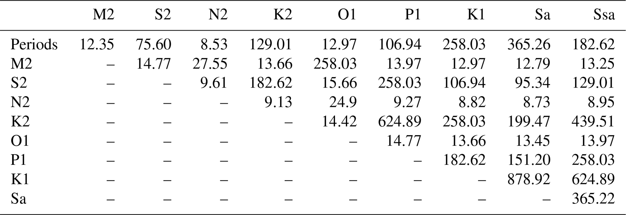
Like the barotropic tides, the internal tides are a mixture of long- and short-period waves, among which are the main astronomical tides, such as the diurnal waves (O1, K1, P1) and the semidiurnal waves (M2, S2, N2, K2). Due to the long repeat cycles of altimetry satellites, short tidal periods are aliased to longer periods (Le Provost, 2001). The M2 tide, for example, is aliased to 62.11 d for the TOPEX/Jason 10 d orbit (9.92 d precisely). With SWOT sampling, M2 is aliased to 66.02 d or 12.35 d (Table 1), depending on whether we consider the 21 d final science orbit or the 1 d calibration/validation (Cal/Val) orbit (0.99343 d exactly). Table 1 gives an overview of the aliasing periods of the main diurnal and semidiurnal tidal frequencies on the SWOT Cal/Val orbit. Table 1 is completed by the Rayleigh criterion values which provide information on the duration of the records needed to separate the different waves. SWOT was maintained in its Cal/Val orbit for about 6 months, providing slightly more than 3 months of usable data from March to early July 2023. Our study is based on this unprecedented 1 d orbit database and concerns observations along a single SWOT track in the Atlantic Ocean.

Table 1 Period of aliasing (in days, second row) and separability following the Rayleigh criterion (in days, from the third row to the end) of main tidal waves for SWOT's 1 d orbit.

This study focuses on Cal/Val track  20 off the Amazon shelf in the western tropical Atlantic between 2° S and 15° N (Fig. 1). The track has been chosen because the Amazon shelf is one of the hot spots for internal tide generation in the ocean (Arbic et al., 2012; Solano et al., 2023; Niwa and Hibiya, 2011). The region is marked by strong seasonal cycles of stratification, circulation, and eddies that regulate the generation and propagation of internal tides (Barbot et al., 2021; Tchilibou et al., 2022). The stratification is modulated by freshwater inflows from precipitation (under the Intertropical Convergence Zone) and rivers (Amazon and Para rivers). The strong western boundary current, the North Brazil Current (NBC), controls the extension of the Amazon's plume and develops a double retroflexion into the Equatorial UnderCurrent (EUC, around 2° S–2° N) and the North Equatorial CounterCurrent (NECC, around 5–8° N). The barotropic and baroclinic instabilities of these currents generate some of the eddies present in the region (Aguedjou et al., 2019). Internal tides generated between the isobaths 100 and 2000 m along the shelf break propagate mainly from the six sites indicated in Fig. 1 (Tchilibou et al., 2022; Assene et al., 2024). Between March and July, the pycnocline is shallow; the mesoscale activity and currents are weak; and, consequently, internal tides tend to be more coherent (Tchilibou et al., 2022). During the rest of the year, the pycnocline is deeper; mesoscale activity and currents are strong; and, consequently, the incoherence of internal tides increases as their reflection and advection by the circulation intensifies. As they evolve, internal tides disintegrate into nonlinear internal solitary waves (Jackson et al., 2012; Alford et al., 2015; Egbert and Erofeeva, 2021). Packets of nonlinear internal solitary waves (ISWs) have been reported along the Amazon continental shelf and offshore (Lentini et al., 2016; Bai et al., 2021; Brandt et al., 2002; Magalhaes et al., 2016). They are highly active in the area (4–8° N and 40–45° W; see Fig. 2 of de Macedo et al., 2023) of concentration of internal tide rays emanating from sites A and D, and they have a seasonal cycle of occurrence and wavelengths in agreement with those of internal waves (de Macedo et al., 2023).

The orientation of SWOT track 20 in this part of the ocean is such that it intersects three areas with potentially different dynamics (Tchilibou et al., 2022). Between 2.5° S and 2.5° N (area 1, Fig. 1), the track is in the path of internal tides generated at points B, C, and (to a lesser extent) A. In area 2, between 2.5 and 8° N (Fig. 1), the track crosses the zone of interaction between internal tides and mesoscale activity. Finally, area 3, north of 10° N (Fig. 1), lies on the Mid-Atlantic Ridge, where some ITs can also likely be generated. We will keep all this in mind when interpreting our results.

The paper is structured as follows. The data used, the evidence for the presence of internal tides in the SWOT data, and the variability of the sea level anomaly (SLA) at different scales are presented in Sect. 2. The amplitude of the internal tides is first estimated from the SWOT data in Sect. 3. In Sect. 4, the estimation of internal tides is improved by introducing PCA. The SWOT-based internal tide models and HRET are further compared in Sect. 5. The paper ends with a conclusion and discussion.

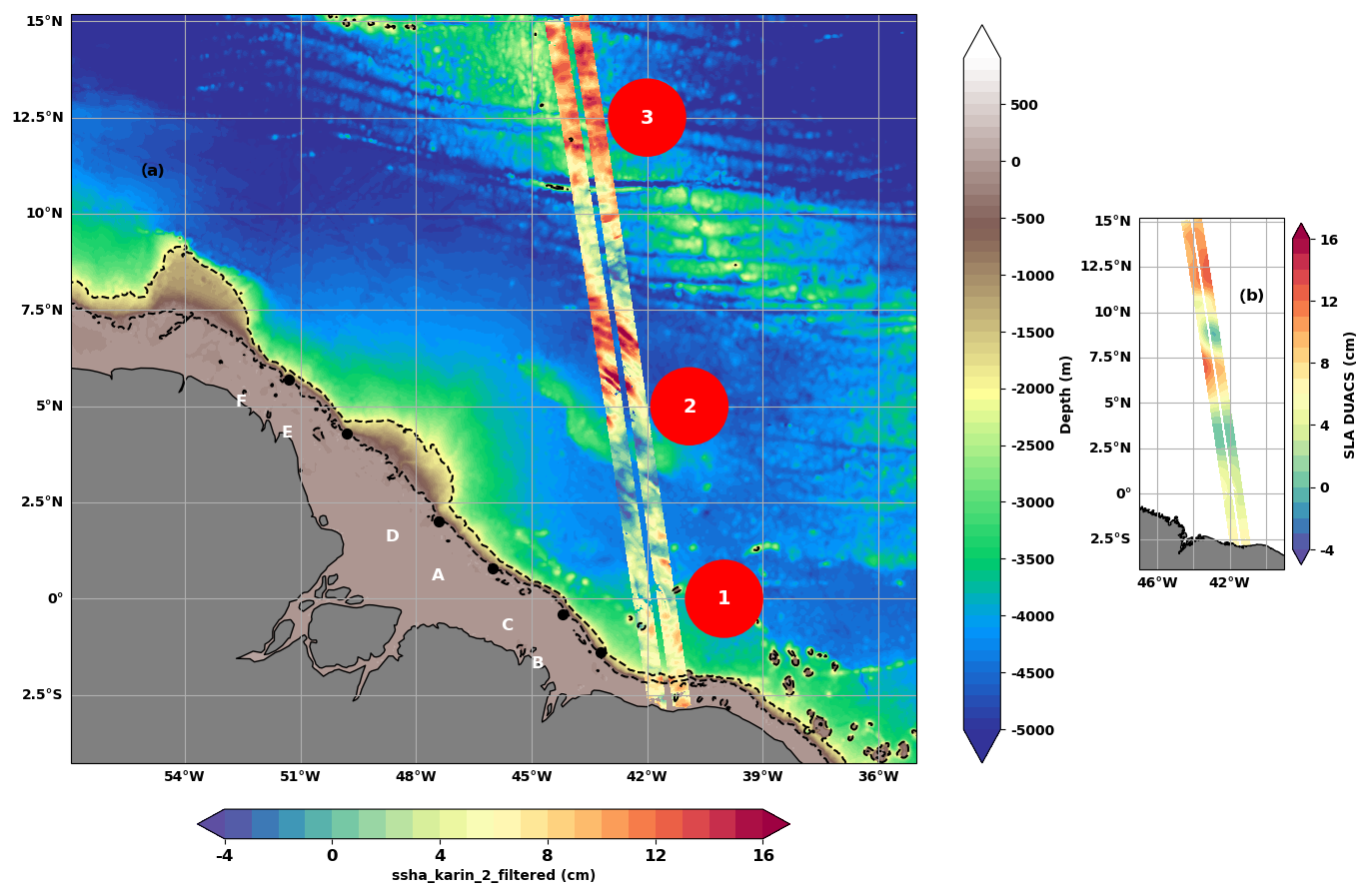
Figure 1 (a) Bathymetry (m) off the Amazon shelf in the western tropical Atlantic. SLA KaRIn (cm) on 8 April 2023, along track 20 of SWOT's 1 d cycle. The main internal tide generation sites are marked by the letters A to F. The 200 and 2000 m isobaths are shown as dashed lines. The circles identify area 1 (2.5° S to 2.5° N), area 2 (2.5 to 8° N), and area 3 (north of 10° N) along the track. (b) Large-scale structure from DUACS on the same date.

2 Data and variability: evidence of IT propagation at different scales

2.1 Description of the database

We use the V0.3 version of the level 3 (L3) SWOT products, published in December 2023 on the AVISO website (CNES, 2023) and CNES Cluster website (Centre National d'Etudes Spatiales). The data, made up of several variables, are provided on regular horizontal grids of 2 km by 2 km. Using the naming convention used in the CNES Cluster dataset, we have defined the SLA by Eq. (1) below:

$$\begin{array}{}\text{(1)}& \begin{array}{rl}\mathrm{SLA}& =\mathrm{ssha}\mathrm{\_}\mathrm{karin}\mathrm{\_}\mathrm{2}\mathrm{\_}\mathrm{filtered}+\mathrm{internal}\mathrm{\_}\mathrm{tide}\mathrm{\_}\mathrm{hret}\\ & -\mathrm{duacs}\mathrm{\_}\mathrm{ssha}\mathrm{\_}\mathrm{karin}\mathrm{\_}\mathrm{2}\mathrm{\_}\mathrm{oi}.\end{array}\end{array}$$

The first term on the right, “ssha_karin_2_filtered” (the same as ssha_noiseless on the AVISO website), is the SWOT observation at the two KaRIn swaths only. We exclude SWOT nadir observations to focus on SWOT's potential to directly observe 2D maps of the ocean. The ssha_karin_2_filtered signal has been denoised using data-driven machine-learning noise reduction and corrected from all the classic physical, instrumental, and environmental corrections applied in altimetry (Dibarboure et al., 2024). The tidal corrections applied are the FES2022 model (Florent Lyard, personal communication, 2024; Lyard et al., 2021) for the barotropic tide and HRET for the internal tide (Zaron, 2019). We reintroduced HRET's internal tide SSH (internal_tide_hret) so that our final SLA contains the total internal tide signal. The last term “duacs_ssha_karin_ 2_oi” corresponds to the DUACS (Data Unification and Altimeter Combination System) maps of sea level anomaly (MSLA) interpolated on SWOT swaths (Ballarotta et al., 2023; Ubelmann et al., 2015, 2021). It removes the large-scale ocean signals and particularly the mesoscale eddies that can mask internal waves at these latitudes. On track 20, we have the SLA from 29 March to 10 July 2023, i.e. 104 cycles with completely or partially filled swaths. We have removed the mean SLA from the entire Cal/Val mission.

We recall that HRET is an empirical estimate of the internal tides at the M2, S2, K1, and O1 frequencies. The variable internal_tide_hret in the SWOT data and HRET model in this paper refers to the HRETv8.1 version (Zaron, 2019). This version was developed by analysing 25 years (1993–2017) of exact-repeat mission altimetry including the TOPEX/Poseidon-Jason missions, the ERS-Envisat-AltiKa missions, and the GEOSAT Follow-On mission. The implementation of HRET involves a local two-dimensional Fourier analysis of the along-track data and the determination of the coefficients of a spatial model by weighted least-squares fitting (second-order polynomial fitting). The estimated tidal fields are gridded on a regular latitude–longitude grid by weighted averaging, and a mask is used to set the values to zero in regions where the estimate is too noisy. HRET includes mode 1 and mode 2 internal tides, but mode 2 is very weak in the present study area.

2.2 Evidence of IT propagation at different scales

The snapshots in Fig. 2a show very fine-scale crest-like structures superimposed on positive and negative SLA, spaced tens and hundreds of kilometres apart. The scenario repeats itself in the other cycles (see the animations in the Supplement), indicating that SWOT likely sees internal waves of different spatial scales. We subjected the SLA to a spectral analysis to find out more about its frequency and wavelength content. The 2D FFT (fast Fourier transform) spectra are computed in the time (cycles) and along-track (latitude) dimensions and then averaged over the cross-track (longitude) dimension. A 25 % cosine taper window or Tukey 0.25 window is used for windowing. The wavenumber–frequency signal (Fig. 3a) was integrated to derive the wavenumber spectrum (Fig. 3b) and the frequency spectrum (Fig. 3c).

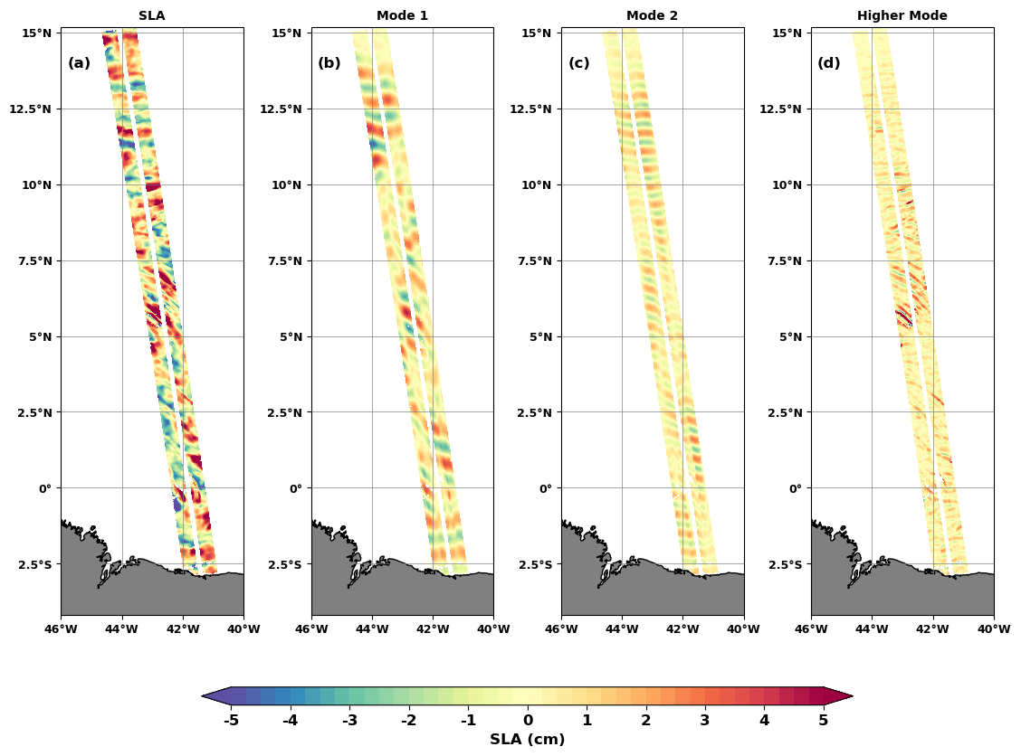
Figure 2 Snapshot of SWOT SLA on 8 April 2023. (a) Total SLA, (b) mode 1 FFT-filtered SLA (180–90 km), (c) mode 2 FFT-filtered SLA (80–60 km), and (d) higher-mode FFT-filtered SLA (50–2 km).

The wavenumber–frequency (Fig. 3a), the wavenumber (Fig. 3b), and the frequency (Fig. 3c) spectra of SWOT SLA indicate that the dominant signal is M2, aliased to 12.22 d (see Table 1). At the M2 aliased frequency, the energy is greatest between 180–90 km and between 80–60 km (Fig. 3a), leading to the spectral peaks in Fig. 3b. These two wavelength bands correspond well to the theoretical baroclinic mode 1 and mode 2 scales expected for the internal tide in this region (Zhao, 2021). We isolated the SLA for these two wavelength bands using FFT filtering. When filtering, the FFT is calculated on the along-track dimension. Snapshots of the mode 1 and mode 2 SLA are shown in Fig. 2b and c for the same day as Fig. 2a, revealing more of the SLA's wavelike behaviour.

Figure 2d shows the FFT-filtered SLA between 50–2 km. This band contains all the small-scale structures, including the very remarkable and intense one that appears as wave crests on the SLA. On the wavenumber–frequency spectrum (Fig. 3a), the energy maximum at frequency M2 extends to scales smaller than 50 km. According to Barbot et al. (2021), this could be associated with the internal tide of mode 3, mode 4, and mode 5. We therefore consider the 50–2 km band as consisting of higher modes.

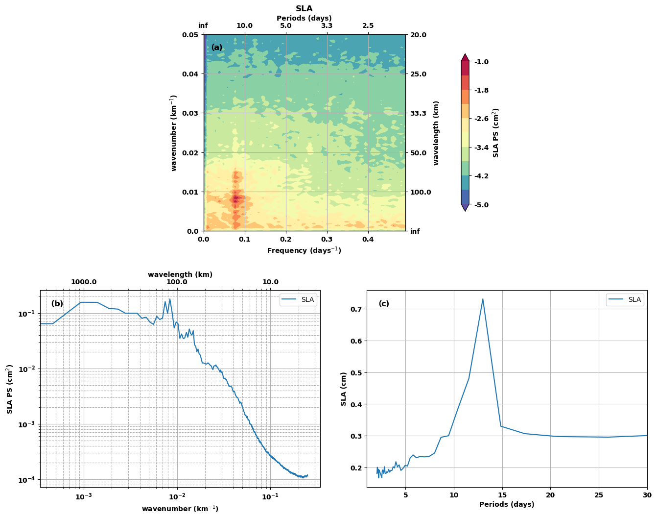
Figure 3 (a) Wavenumber–frequency, (b) wavenumber, and (c) frequency spectra of the total SLA.

2.3 Variability analysis of IT observations

Analyses of SLA variability are completed by calculating the standard deviations of the total and the spatially FFT-filtered SLAs in the wavelength bands defined above. Over the Cal/Val period, SLA varies between 1 and 5 cm under track 20 (Fig. 4a). Apart from the area very close to the coastline, there are three main patches of maximum variability, each located in one of the dynamic areas highlighted in the Introduction. The maximum variability of the SLA in area 1 (2.5° S–2.5° N) is mainly due to the regular mode 1 internal tide flux likely coming from sites A, B, and C (Fig. 4b). Mode 2 and higher-mode contributions are secondary (Fig. 4c and d) in area 1. Higher modes have a major impact on the variability in area 2 where they make the SLA vary by 2 to 3 cm (Fig. 4d), i.e. almost of the same order as mode 1 in the same area. As area 2 is far from the generation sites of the Amazonian shelf break, the higher modes here are likely to originate from disintegration of mode 1 and mode 2. In area 3, SLA variability is driven mainly by mode 1 and mode 2.

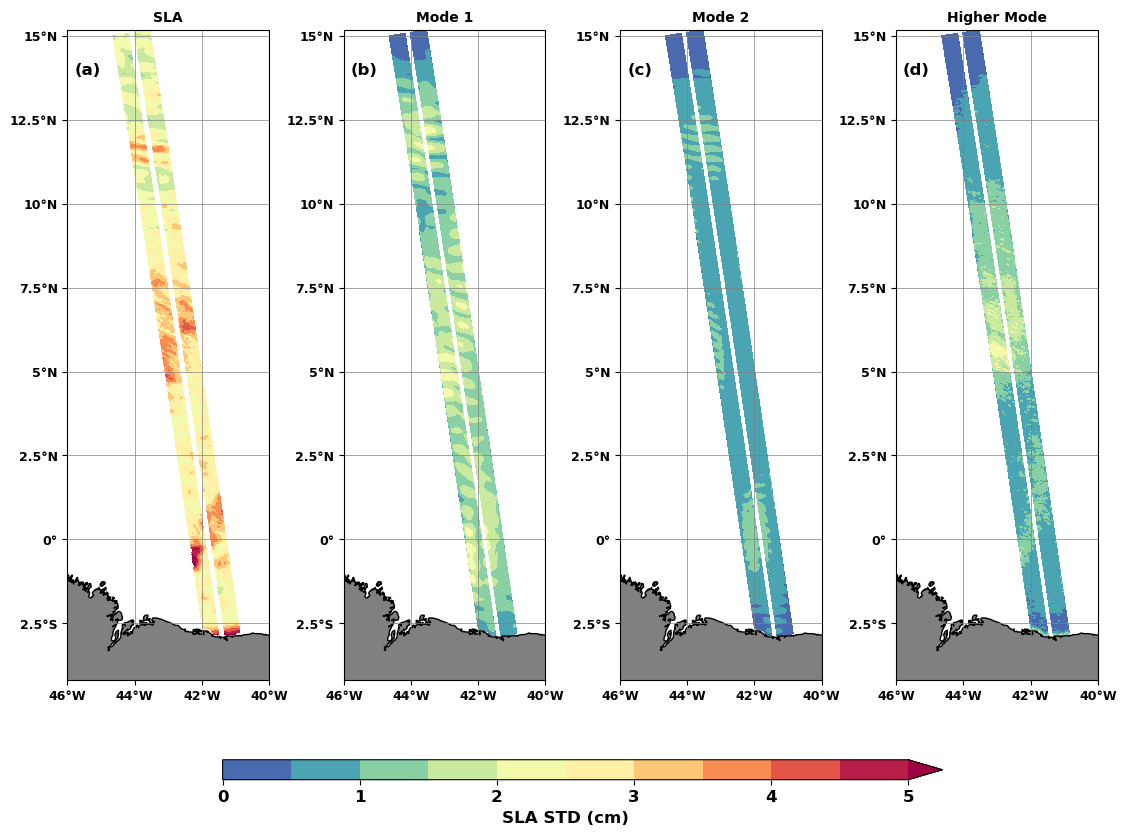
Figure 4 Standard deviation (in cm) of the total SLA (a) and mode 1 (b), mode 2 (c), and higher-mode (d) FFT-filtered SLAs.

3 The M2, S2, and N2 coherent internal tides from SWOT: the ITkars model

In Table 1, four waves (M2, N2, S2, and O1) have aliasing periods shorter than the 104 d corresponding to the total length of our SWOT SLA series and are of interest for our analysis. But given the Rayleigh criterion between them in Table 1, it is reasonable to restrict ourselves to the three semidiurnal waves. Harmonic analysis based on least-squares fitting is used to extract the coherent internal tide at each band point with at least 80 valid cycles over the entire SWOT Cal/Val observation period. In the following, ITkars (IT from KaRIn SWOT) refers to the SWOT estimation of IT.

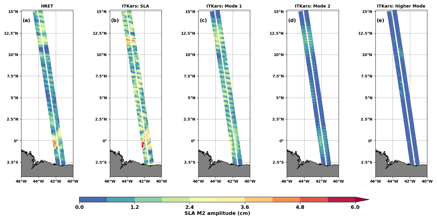
Figure 5 The amplitude (in cm) of the M2 internal tide from the HRET model (a) and the ITkars model (b–e) over the Cal/Val period. ITkars is derived by harmonic analysis of the total SWOT SLA (b) and FFT-filtered SWOT SLA for mode 1 (c), mode 2 (d), and higher-mode (e) SLAs. Only swath points with at least 80 valid cycles were analysed.

The amplitudes of the coherent internal tide at the M2 frequency are presented in Fig. 5 for both HRET (which include mostly mode 1 in this area) and ITkars models (which include mode 1 and mode 2). We first performed the harmonic analysis of the total SLA (Fig. 5b) and repeated the harmonic analyses for each of the FFT-filtered SLAs (Fig. 5c–e). The HRET model (Fig. 5a) and the ITkars model based on the total SLA (Fig. 5b) are similar in terms of spatial distribution, but as expected HRET has smoother and lower amplitudes because it represents a mean on many years of altimetry data. In areas 1 and 3, ITkars shows spatial features identical to those already observed in the standard deviation in Fig. 4a. So, the maximum variability for these two parts of the SWOT track is indeed due to the M2 coherent internal tide. The discrepancies between standard deviations (Fig. 4) and internal tide amplitudes (Fig. 5) are best seen by directly comparing the maps for the different modes or wavelength bands. In area 2, the amplitude of the coherent internal tide is less than 1.5 cm for the higher modes (Fig. 5e), whereas at these scales the standard deviation is maximal (Fig. 4d). The high variability of the SLA found in area 2 is evidently related to internal tide incoherency.

As S2 from HRET shows unexpected patterns (not shown) and as N2 is not available in HRET, we show only ITkars results in Fig. 6. Both waves have smaller amplitudes than M2 and do not have the same structure as the latter. As the semidiurnal S2 and N2 ITs should have similar patterns to M2, those results indicate that these frequencies are certainly contaminated by other tidal waves due to poor separability on the available period (see Table 1) and are likely also contaminated by the mesoscale activity. Can we hope to improve our estimate of the coherent internal tide from SWOT observations?

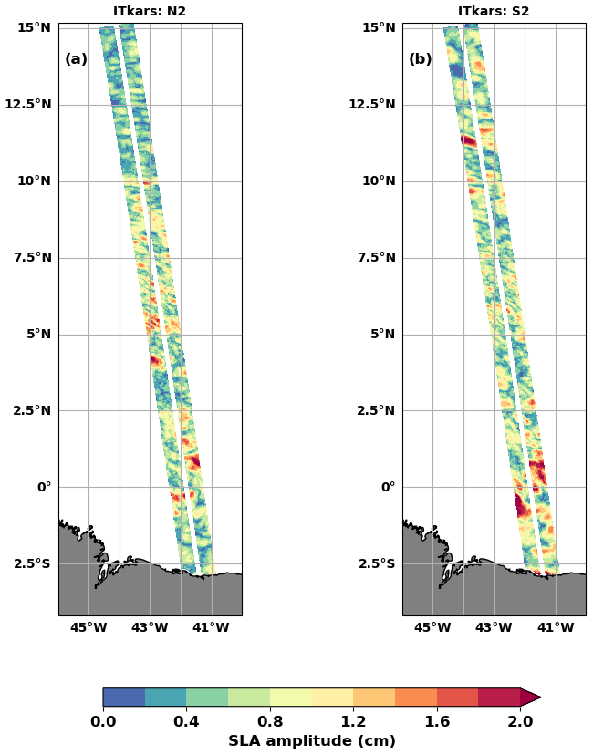
Figure 6 The amplitude (in cm) of the N2 (a) and S2 (b) internal tides of the ITkars model derived by harmonic analysis of the total SLA over the Cal/Val period. Only swath points with at least 80 valid cycles were analysed.

4 An attempt to improve the estimation of coherent internal tide from SWOT Cal/Val data using principal component analysis (PCA) to separate SLA content

4.1 Separation using PCA

PCA, also known as EOF (empirical orthogonal function) analysis, is a statistical analysis technique for reducing the dimensionality of a dataset (Jolliffe, 1986). Applied to geophysical data, PCA separates the total signal into independent spatial patterns associated with independent temporal components (principal components, PCs) and gives a measure of the relative importance of each pattern (a percentage of the total variance). The first PCs capture most of the variance in the data and generally have a repetitive and persistent structure, thus behaving approximately like the stationary component of the signal. In particular, coherent internal tides have significant spatial correlations that PCA could identify and isolate. On this basis, we believe that PCA applied to our total SLA can help better isolate the coherent internal tide (which is stationary) from the remaining residual tidal (incoherent internal tides) and non-tidal signals observed by SWOT. Egbert and Erofeeva (2021) have successfully used PCA to determine the characteristics of the incoherent internal tide around the Amazon shelf. In this paper, we focus on the coherent internal tide. Therefore, we performed the PCA on the 104 cycles of the SWOT KaRIn total SLA as defined in Eq. (1). At each point in the swath, we filled in the missing value with the local time mean and then normalized the SLA to ensure that the global mean and standard deviation become zero and one, respectively. The covariance matrix is calculated on the normalized SLA; the PCA focuses on eigenvalues and not absolute values.

The two leading PCA modes shown in Fig. 7 account for 14.05 % (PCA1, Fig. 7a and c) and 10.46 % (PCA2, Fig. 7b and d) of the total variance. Their spatial patterns correspond to IT structures: for PCA1 (Fig. 7a) the IT is intensified in area 1 and area 3, while PCA2 (Fig. 7c) is characterized by an increase in the IT intensity in area 2. PCs show 12–13 d oscillations with modulations around 70 d (Fig. 7b and d), therefore recalling the aliasing periods of M2 and S2 waves (see Table 1). To get a more precise idea of the wavelengths and frequencies contained in PCA1 and PCA2, we reconstructed the SLA for both components (SLA_pca1 and SLA_pca2) and calculated the spectra shown in Fig. 8 (blue line for PCA1 and orange line for PCA2).

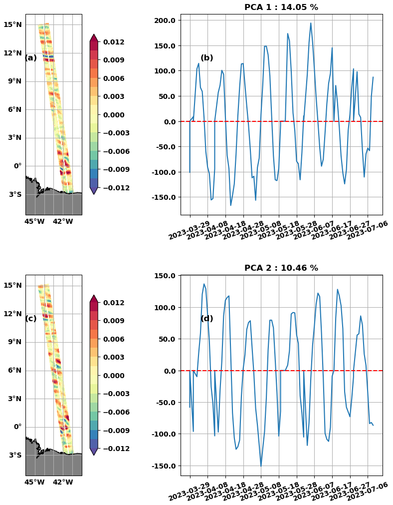
Figure 7 Spatial (a, c) and principal (b, d) components of PCA1 (a, b) and PCA2 (c, d) of the SLA along SWOT swaths over the Cal/Val period.

The wavenumber spectra (Fig. 8a) indicate that PCA1 and PCA2 consist mainly of mode 1 (180–90 km) and mode 2 (80–60 km) ITs. A peak that could be associated with mode 3 stands out in the PCA2 spectrum, but overall, the energy levels of both spectra remain low for higher modes (50–2 km). The frequency spectra (Fig. 8b) confirm that M2 is the dominant signal. At this frequency, the mean SLA amplitudes are 0.52 cm for PCA1 and 0.45 cm for PCA2, respectively, 71 % and 61 % of the 0.73 cm associated with the peak of the total SLA reported by the solid black line in Fig. 8b. Amplitudes are low for other frequencies. The 104 available cycles are not enough to observe 70 d modulation in the frequency spectra. Given the wavenumber and frequency spectra, we can say that PCA1 and PCA2 are two complementary representations of the propagation and evolution of the M2 dominant internal tide, so they can be merged to form a single signal. We have summed SLA_pca1 and SLA_pca2 into SLA_pca_L2 (L2 refers to lower or equal to 2). A snapshot of SLA_pca_L2 is shown in Fig. 9a for the same cycle as in Fig. 2. Interestingly, the SLA reconstructed with PCA1 and PCA2 have similar patterns to the mode 1 and mode 2 FFT-filtered SLAs (Fig. 2b and c).

Between PCA3 and PCA10, the variance explained is less than 3.58 % per PCA; from PCA11 onwards, the variance becomes less than 2 % (not shown). The PCs are a mixture of several wave frequencies, with M2 of lower intensity than in PCA1 and PCA2, high frequency (faster than 10 d) and low frequency (15, 17, or even 25 d). It is difficult to associate the spatial patterns of these PCs with the propagation of a persistent IT in time and along the track or even with a mode of ocean variability to our knowledge. The last three PCA patterns resemble residual noise from the processing of raw SWOT data. We grouped PCA3 to PCA104 into SLA_pca_G2 (G2 for greater than 2). The small-scale structures that were identified in Fig. 2a are clearly visible in the snapshot of the SLA_pca_G2 in Fig. 9b. Figure 9a and b are complementary, as the PCA acted as a filter. The total SLA is now split into SLA_pca_L2 and SLA_pca_G2. The spectra of SLA_ pca_G2 are shown in green in Fig. 8. Nearly all energies for scales above 180 km (seen as large scale) and below 50 km (for higher modes) are found in the wavenumber spectrum of SLA_pca_G2. Around the aliased frequency of M2, the mean amplitude is 0.19 cm for SLA_pca_G2. This is about a quarter of the mean amplitude of the total SLA (0.73 cm). With such a drop in the energy of the spectrum, PCA acted as the classic detiding (removal of tidal variability) SLA – ITkars. To verify this, we calculated the spectra of the total SLA detided with M2 from ITkars and plotted them as a dashed black line in Fig. 8. At all frequencies and wavelengths, they overlap well with the spectra of SLA_pca_G2. Therefore, SLA_pca_G2 is more representative of the incoherent internal tide, and SLA_pca_L2 is more suitable for improving the estimation of the coherent internal tide.

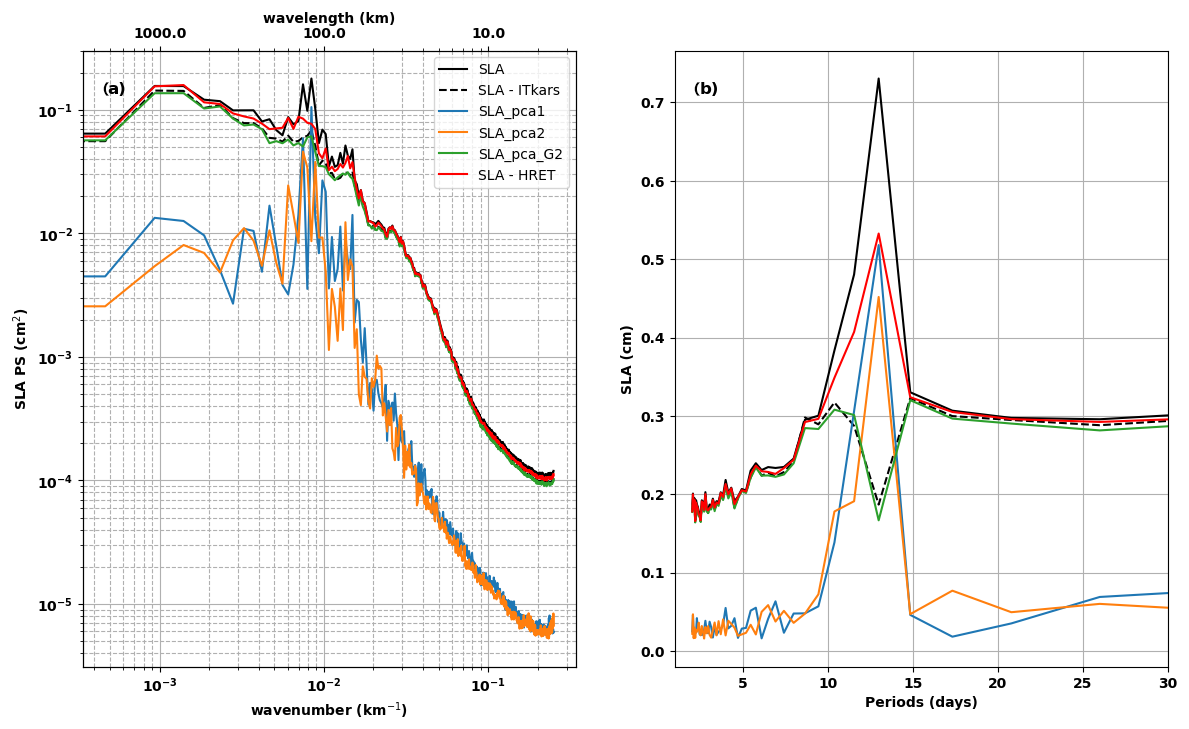
Figure 8 Wavenumber (a) and frequency (b) spectra of SLA_pca1 (in blue), SLA_pca2 (in orange), SLA_pca_G2 (in green), SLA – HRET (in red), and SLA – ITkars (black dashed line). SLA_pca_G2 is the sum of the SLAs of PCs greater than 2. The spectra of total SLA (solid black line) from Fig. 3 are reported here. ITkars is the internal tide model derived from the SWOT KaRIn data (see Sect. 3).

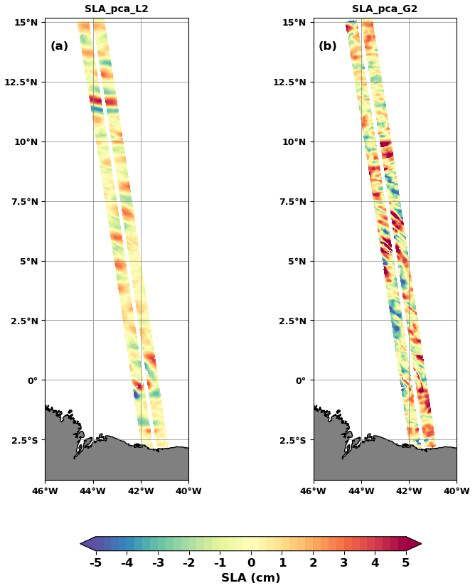
Figure 9 Snapshot of SWOT SLA_pca_L2 (a) and SLA_pca_G2 (b) on 8 April 2023 (as in Fig. 2). SLA_pca_L2 is the sum of the SLAs of PCs less than or equal to 2 (PC1 and PC2).

4.2 ITkars_pca internal tide model

We have performed the harmonic analysis of SLA_pca_L2 at the semidiurnal frequencies M2, N2, and S2 (Fig. 10). The resulting internal tide amplitude (model) is referred to as ITkars_pca to distinguish it from ITkars based solely on harmonic analysis of SWOT KaRIn data. Compared to Fig. 6 (corresponding to ITkars), the ITkars_pca internal tide maps for N2 (Fig. 10a) and S2 (Fig. 10b) are cleared of small scales, and the patterns for both waves are now close to that of M2 as expected (Figs. 10c and 5b reported in Fig. 10f). At first glance, there seems to be no difference between ITkars (Figs. 5b or 10f) and ITkars_pca (Fig. 10c) for M2. By making the complex difference between the two signals (Fig. 10c and f), we deduce the amplitude shown in Fig. 10d, which is equivalent to the amplitude of the harmonic analysis of SLA_pca_G2 at M2. As with N2 and S2, Fig. 10d shows that M2 ITkars (Figs. 5b or 10f) also contains an additional signal dominated by small scales and which does not resemble the classic internal tide.

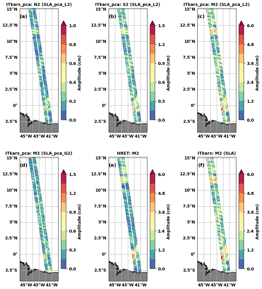
Figure 10 The amplitude (in cm) of the internal tides N2 (a), S2 (b), and M2 (c, d) of the ITkars_pca model derived by harmonic analysis of SLA_pca_L2 (a–c) and SLA_pca_G2 (d) over the Cal/Val period. SLA_pca_L2 is the SLA based on PCA1 and PCA2; SLA_pca_G2 is compiled from PCA3 to PCA104. Only swath points with at least 80 valid cycles were analysed. Figure 5a and b are reported here, i.e. M2 HRET (e) and M2 ITkars (f).

The origin of the extra signal contaminating ITkars could be dynamic or numerical. Dynamically, these could be very intense nonlinear waves, solitons, or incoherent internal tides, which are retained in the harmonic analysis of Sect. 3 due to the short length of the time series. On the numerical side, noise linked to the pre-processing of SWOT data cannot be ruled out. Another source of contamination could also be the DUACS correction we apply beforehand to distinguish internal tides.

5 Complementary comparison between SWOT and HRET IT models: predictability of internal tides

The comparison between HRET- and SWOT-based internal tide models (ITkars and ITkars_pca) is taken a step further in this final section. Each of the atlases (amplitude and phase) will be used as an internal tide correction model for the SWOT data. This involves making internal tide predictions over a given period and then subtracting these predictions from raw observations. Various metrics are used to quantify the capability of each model to reduce the variance.

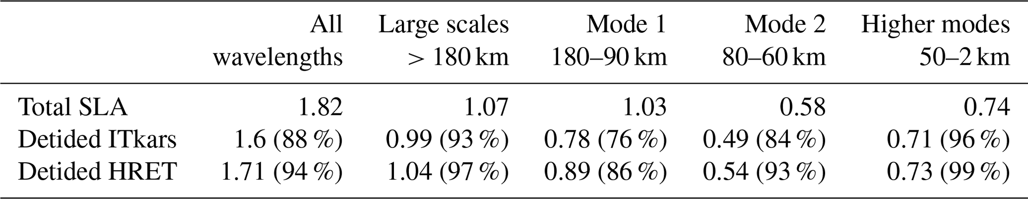
In Fig. 8, the ITkars M2 atlas has been used as a correction model to detide the total SLA over the entire Cal/Val observation period (dashed black line). We have done the same with M2 from HRET, and the corresponding spectra are shown in red in Fig. 8. As in Fig. 3, the 1D spectra are integrations of the 2D wavenumber–frequency spectrum. On the wavenumber spectra, the peaks of mode 1 and mode 2 are reduced but remain visible whatever the detiding applied (Fig. 8a). We have integrated the wavenumber spectra of the total SLA (black line in Fig. 8) and the detided SLA (dashed black and red lines in Fig. 8) over all wavelengths, between 180 and 90 km for mode 1, between 80 and 60 km for mode 2, from 50 to 2 km for the higher modes, and finally over wavelengths greater than 180 km for the large scale. The derived standard deviations are presented in Table 2 for the total SLA and the SLA detided with ITkars or HRET, as well as the percentages expressing the residual variance rate (ratio of the variances of the detided SLA on the total SLA). The higher the standard deviation of the detided SLA (or the percentage in Table 2), the less efficient the correction used for detiding. According to Table 2, the application of the M2 internal tide prediction of each of the models removes very little variance from the SLA; nevertheless, ITkars is more efficient than HRET, especially at mode 1 and mode 2 scales. For these scales, the residual variance reaches 76 % and 84 % of the SLA after correction by ITkars and is likely to be an incoherent internal tide. For the higher modes, Table 2 agrees with Fig. 5e: the M2 correction has no effect on these scales. ITkars has a greater impact on large-scale SLAs than HRET: HRET has almost no signal at large scale by construction, while ITkars can capture some variability at large scales due to short time series and no fitting approximation. When detiding with ITkars, the energy spectrum (Fig. 8b) decreases strongly around the aliased frequency of M2 (around 13 d; see Table 1). The mean of SLA amplitude along the SWOT swaths drops by 74 % (from 0.73 to 0.19 cm) after ITkars detiding at the M2 frequency. With the HRET correction (Fig. 8), the peak amplitude at the M2 frequency is 0.53 cm, i.e. a 27 % reduction of the peak of the total SLA, which is more than twice lower than with the ITkars correction. It can also be seen that periods of more than 15 d and less than 5 d are not affected by the correction, since we have limited ourselves to the M2 frequency.

Table 2 Comparative table of the standard deviations of total SLA and SLA detided with HRET or ITkars. Standard deviations are obtained by integrating the spectra of Fig. 3c over different wavelength bands (in cm). The ratio between detided SLA and total SLA, computed as a percentage, is given in parentheses.

The better performance of the ITkars correction in comparison to HRET is not surprising, since ITkars is derived from the same database to which the detiding is applied. The result is almost identical to ITkars when the SLA is detided with M2 from ITkars_pca. This is not surprising as the amplitude of the M2 residual in SLA_pca_G2 is small (Fig. 10d). To obtain the best possible comparison between ITkars and ITkars_pca while still focusing on the M2 wave, we propose to apply the detiding to data that are independent of those used to derive the internal tide atlas. Thus, the SWOT data were divided into two periods: period 1, comprising the first 70 cycles (from late March to early June), and period 2 (from early June to early July), comprising the last 34 cycles. We repeated the M2 harmonic analysis of the total SLA over period 1 and derived the atlas “ITkars_p1” (p1 indicates period 1). We did the same with SLA_pca_L2 and derived the atlas “ITkars_pca_p1”. The atlases ITkars_p1, ITkars_pca_p1, and HRET are then used to detide the SLA and SLA_pca_L2, firstly in period 1 and secondly in period 2, which is independent of period 1. Since period 2 is short for frequency spectral analysis, we are going to look at the standard deviation (Table 3) and the variance reduction (Fig. 11). Variance reduction is calculated from Eq. 2 as the difference between the variance of corrected SLA and the variance of the uncorrected SLA (or SLA_pca_L2). A negative variance reduction indicates that the internal tide correction reduces the SLA variance.

$$\begin{array}{}\text{(2)}& \text{Variance reduction}=\mathrm{var}(\mathrm{SLA}-\text{M2 atlas})-\text{var (SLA)}\end{array}$$

The spatial mean of the standard deviation is summarized in Table 3. For period 1, the standard deviation of the total SLA is 2.56 cm. After correction with M2 of the HRET model, the standard deviation drops by 7 % (to 2.39 cm). The SLA standard deviation decreases by about 15 % and 14 % with ITkars_p1 and ITkars_pca_p1, respectively. The difference between the two ITkars models is not significant as we detide the same data that are used to derive the models (ITkars_p1 in particular). The application of the corrections to SLA_pca_L2 reduces the residual standard deviation from 1.33 to 0.99 cm for HRET, to 0.53 cm for ITkars_p1, and to 0.42 cm for ITkars_pca_p1. This shows that even in an SLA dominated by coherent internal tides, HRET removes only 15 % of the variance, whereas SWOT-based internal tide models remove over 60 %. ITkars_pca_p1 is obviously the best correction for SLA_pca_L2, with ITkars_p1 being slightly less efficient.

For period 2, the corrections of the SLA with the three internal tide models are less efficient. Table 3 shows that, on average, between 5 % and 9 % of the SLA variance is suppressed, with ITkars_pca_p1 being the best corrective internal tide model. As can be seen from the variance reduction maps (Fig. 11a–c), the three models reduce variance (blue colour) in the parts of the swath where the coherent internal tide signal is strong enough (Fig. 10). Outside these areas, the internal tide models tend to add variance, and the variance reductions become positive. This undesirable effect of the correction models is mainly observed in the central part of the swath (area 2), where the higher modes contribute significantly to the SLA variability (see Fig. 4). The effect in area 2 is pronounced for ITkars_p1 (Fig. 11b), indicating a prediction failure. When considering the independent SLA_pca_L2 data (period 2, Table 3), HRET removes 21 % of the variance. For ITkars_p1 and ITkars_pca_p1, the variance is reduced by 45 % and 55 %, respectively. The impact of PCA on the derivation of the M2 internal tide atlas is highlighted here by the 10 % gap between the percentages of variance reduction when applying the two models based on SWOT observations. The variance reduction figures confirm that the correction works better on SLA_pca_L2 (Fig. 11d– e). Although there are still swath locations with positive variance reduction, this is no longer concentrated in the central part. Variance reductions are dominated by negative values for ITkars_p1 (Fig. 11e) and ITkars_pca_p1 (Fig. 11f).

Table 3 Comparative table of standard deviations (cm) of SLA and SLA_pca_L2 detided with either M2 HRET, M2 ITkars, or M2 ITkars_pca models over period 1 (from late March to early June 2023, the first 70 cycles) and period 2 (from early June to early July 2023, the last 34 cycles). The ITkars_p1 and ITkars_pca_p1 models were built with period 1 and validated with period 2. The ratio between detided SLA and total SLA is indicated in the parentheses (in percent).

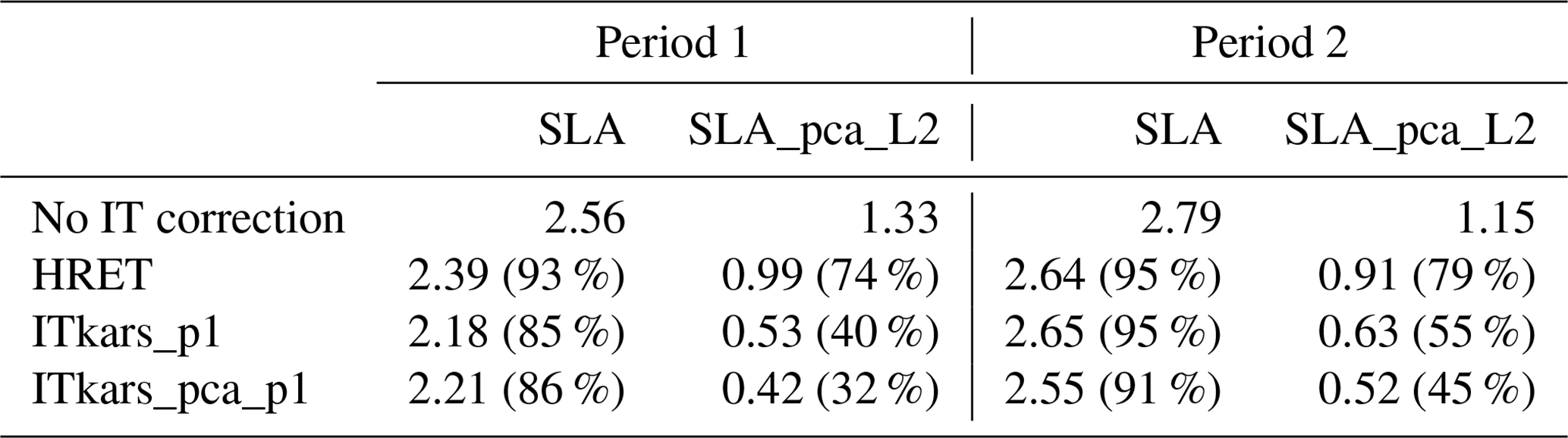
Figure 11 Variance reduction of SWOT SLA (in cm²) in period 2 from early June to early July (last 34 cycles) when using either M2 HRET (a, d), M2 ITkars_p1 (b, e), or M2 ITkars_pca_p1 (right column) to correct the total SLA (a, b, c) or SLA_pca_L2 (SLA_L2 in the title; d, e, f) and compared to the no IT correction case.

6 Discussion and perspectives

In this study, we explored and characterized the internal tide signal in SWOT KaRIn observations over the Cal/Val period (1 d orbit) between late March and early July 2023 (104 cycles) and along track 20, located off the Amazon shelf in the tropical Atlantic between 2° S and 15° N. The internal tide as seen by SWOT is a mixture of several spatial scales, including baroclinic modes 1 and 2 defined by wavelengths between 180–90 and 80–60 km, respectively. SWOT also sees very intense fine-scale structures (wavelengths between 50–2 km) that we have associated with higher baroclinic modes, including modes 3, 4, and 5 according to Barbot et al. (2021). As a result, SWOT seems to live up to expectations, providing a direct 2D view of the internal tide sea surface signatures and even access to smaller scales.

Our approach to extract the internal tide signal through the 1 d SWOT data consisted firstly of filtering the large scale (including the mesoscale) by subtracting the DUACS MSLA from the SWOT observations; then we reintroduced the internal tide correction of HRET from Zaron (2019) to obtain a SLA consisting of the total internal tide signal. We either performed the harmonic analysis (as in Sect. 3) or proceeded upstream to the PCA before the harmonic analysis (as in Sect. 4). The internal tide model based on harmonic analysis of SWOT KaRIn data was referenced as ITkars (internal tide from KaRIn SWOT), and the one obtained by combining PCA and harmonic analysis was referenced as ITkars_pca. We focused on the semidiurnal frequencies M2, S2, and N2.

Spatial patterns of M2 internal tides from ITkars and ITkars_pca models agreed with the M2 HRET model based on nearly 25 years of conventional altimeter (nadir) observations. The similarities between models based on SWOT KaRIn and the model with conventional altimeter data are partly linked to the fact that SWOT data are analysed over March to July, during which the internal tide is most stable and coherent off the Amazon shelf (Tchilibou et al., 2022). One consequence of analysing SWOT data over this short 104 d window is that the amplitude of the internal tide is stronger with the SWOT estimation than with HRET. This result is logical since the intensity of the coherent internal tide depends on the length of the time series analysed: a longer time series allows for a better estimate of the coherent signal, which is therefore smoother (Ansong et al., 2015; Zhou et al., 2015; Nash et al., 2012). The separation of M2 from O1 is not ensured with 104 cycles of SWOT 1 d data; however, in this region the amplitude of the internal tide is negligible at the O1 frequency compared to M2 (see Fig. 1 in Tchilibou et al., 2022), so M2 ITkars_pca is thus quite reliable.

The maps of N2 and S2 highlight the contamination of ITkars by signals other than the coherent internal tide, particularly by very small scales. We hypothesize that the contamination is due to the leakage of nonlinear waves, incoherent internal tides, and ocean variability in the harmonic analyses. Regarding ocean variability, part of it is not captured by DUACS and was therefore not subtracted from the SLA. Moreover, subtracting the mesoscale, as we have done, is itself a possible source of error in estimating the internal tide (Zaron and Ray, 2018). One way to reduce the effects of contamination by ocean circulation would be to apply a simultaneous internal tide and mesoscale inversion method as proposed by Ubelmann et al. (2022). The combination of PCA and harmonic analysis gives semidiurnal ITkars_pca maps (M2, S2, and N2) with similar patterns. The amplitude of N2 ITkars_pca deduced from SWOT is of the same order as that in the new product HRET14 (Zaron and Elipot, 2024). The result is encouraging for S2, especially as the length of the 1 d observations is not sufficient to correctly separate it from waves such as Sa and Ssa, whose periods are identical to those of the annual and semiannual variation of the ocean. A longer time series is needed to better separate the internal tide components from SWOT observation, and we will consider analyses of the 21 d SWOT science orbit data when the time series will be long enough.

PCA has improved our estimate of the internal tide model from the SWOT KaRIn data. From the PCA, we kept the first two main modes (PCA1 and PCA2) and considered them as the coherent internal tide given their fairly stationary character. Thus, the coherent internal tide accounts for 24.51 % (14.05 % of PCA1 and 10.46 % of PCA2) of SLA variance in the 1 d SWOT observations, a proportion in line with the studies of Zaron (2017) and Egbert and Erofeeva (2021) in this region. The coherent internal tide isolated through the PCA consists of mode 1, with mode 2 noticeable in PCA1 and PCA2. The fact that the coherent internal tide signal is projected onto two main modes of the PCA is an open question. The principal components of PCA1 and PCA2 are shifted by 3 to 4 d, about a quarter of the aliased frequency of M2, which could correspond to a phase quadrature, as there is between the imaginary and real parts needed to reconstruct a sinusoidal signal. Instead of being the real and imaginary parts of a signal, PCA1 and PCA2 could also represent the same phenomenon and highlight its evolution in area 2 in the middle of the swaths: the moderation of internal tides in area 2 with PCA1 and their intensification with PCA2. This type of PCA/EOF behaviour is observed in the case of El Niño–Southern Oscillation (ENSO) studies in the Pacific (Takahashi et al., 2011). The peaks in the wavenumber spectrum of PCA1 and PCA2 are shifted by few kilometres at the mode 1 and mode 2 scales, suggesting a change in wavelengths relating to changes in stratification conditions as suggested by Barbot et al. (2021). A longer series of Cal/Val observations could have helped to better distinguish PCA1 from PCA2.

The principal components (time series) of PCA1 and PCA2 provide an overview and an opportunity to study the daily variability of internal tide amplitude, a perspective difficult to access with conventional altimetry missions. This opportunity to learn more about the temporal variability of the internal tide using a single high-resolution mission is lost, or at least postponed, with SWOT's switch to its 21 d scientific orbit. One of the limitations of using PCA to analyse SWOT data is probably its sensitivity to track length. The total variance is distributed differently in the principal components depending on whether the track is long or short or whether ocean dynamics change significantly along the track. It would be interesting to look at this point from the perspective of a global model, for example. We are curious to know how the PCA will behave in the case of multi-track use, as well as at their crossing points.

In the context of 1 d SWOT observations, the use of PCA can be useful in determining wave frequencies of interest for the development of the coherent internal tide model. The combination of PCA and harmonic analysis further reveals the observational potential of SWOT. We are currently working on other SWOT tracks in various ocean regions to test the robustness of our method of combining PCA and harmonic analysis. We also plan to explore in situ observations of the SWOT Cal/Val and other databases to better understand our results. Work remains to be done to confirm the presence of mode 3 in the coherent internal tide signal in this region. The incoherence of the internal tide and its interaction with the circulation are other issues to be addressed with these SWOT data.

The final issue addressed in this study was the correction of the internal tide signal in the SWOT 1 d observations. On average, the HRET model corrects only 6 % of the SLA variance over the Cal/Val period, while ITkars based on SWOT observations corrects 12 % (Table 2). These percentages are low due to the high degree of internal tide incoherency in this part of the ocean. However, they indicate that the HRET correction is not efficient enough. It would be more relevant to directly evaluate the internal tide signals on 1 d SWOT observations and then use it as a correction model. The harmonic analysis may be sufficient if the aim is to apply the tidal model to the same data, but if not, the previous step of the PCA is recommended to obtain a more realistic model. The question of correcting internal tides and improving internal tide models will also remain a challenge for the exploitation of SWOT's 21 d cycles.