On the applicability of linear wave theories to simulations on the mid-latitude β-plane

The applicability of one-dimensional (zonally invariant) harmonic and trapped wave theories for Inertia-Gravity waves to simulations on the mid-latitude β-plane is examined by comparing the analytical estimates in the geostrophic adjustment and Ekman adjustment problems with numerical simulations of the linearized rotating shallow water equations. The spatial average of the absolute differences between the theoretical solutions and the simulations, ϵ(t), is calculated for values of the domain's north-south extent, L, ranging from L=4 to L=60 (where L is measured in units of the deformation radius). The comparisons show that: (i) though ϵ oscillates with time, its low-pass filter, ϵ^LP(t), increases with time. (ii) In small domains, ϵ^LP(t) in harmonic theory is significantly smaller than in trapped wave theory, while the opposite occurs in large domains. (iii) The accuracy of the harmonic wave theory decreases with L for $\mathrm{0}<L<\mathrm{20}$, while for L>20 the trend changes with time. (iv) The accuracy of the trapped wave theory increases with L in the geostrophic adjustment problem, while in the Ekman adjustment problem, its best accuracy is obtained when L≈30. (v) There is a range of L and t values for which no theory provides reasonable approximations, and this range is wider in the Ekman adjustment problem than in the geostrophic adjustment problem. Non-linear simulations of a multilayered stratified ocean show that internal inertia-gravity waves exhibit the same characteristics as the wave solutions of the linearized rotating shallow water equations in a single layer ocean.

1 Introduction

The Rotating Shallow Water Equations (RSWE, hereafter) provide a fundamental description of the dynamics of an incompressible fluid in a thin layer in the presence of rotation. This framework is applicable when the horizontal scale of the fluid motion is much larger than the layer thickness. The linear waves of the RSWE include three wave types: Kelvin waves, Inertia-Gravity waves (also known as Poincaré waves) and Planetary waves (also known as Rossby waves). Mid-latitude (coastal) Kelvin waves occur in the presence of an ocean boundary, while all three wave types are generated in response to atmospheric forcing, such as wind stress, or due to local perturbations in the ocean's velocity or surface height. These waves are traditionally classified into two main categories based on their frequencies. The first category comprises the high-frequency Kelvin and Inertia-Gravity waves, which are rotationally modified gravity waves. The second category includes the low-frequency Planetary waves, which originate as perturbations respond to the latitudinal variation of the Coriolis parameter (Gill, 1982; Pedlosky, 1987; Cushman-Roisin and Beckers, 2011, and Vallis, 2017).

In the classical harmonic wave theory in mid-latitudes, the meridional structure of the waves' amplitude is described by harmonic functions, i.e., sine, cosine, or exponential functions. This simple theory provides accurate wave solutions when the Coriolis frequency is assumed constant on a plane tangential to the spherical Earth at some latitude ϕ₀ (i.e., $f=\mathrm{2}\mathrm{\Omega }\sin \left(\mathit{\varphi }\right)\approx f_{\mathrm{0}}=\mathrm{2}\mathrm{\Omega }\sin \left({\mathit{\varphi }}_{\mathrm{0}}\right)$, where Ω is Earth's frequency of rotation). This model is referred to as the f-plane approximation. In contrast, when the Coriolis frequency is assumed to vary linearly with the meridional coordinate y (i.e., $f=f_{\mathrm{0}}+\mathit{\beta }y$, where $\mathit{\beta }=\mathrm{2}\mathrm{\Omega }\cos \left({\mathit{\varphi }}_{\mathrm{0}}\right)/R$ is constant, and R is Earth's mean radius), the model is referred to as the β-plane approximation. On the β-plane, the harmonic wave theory provides only approximate solutions. A detailed derivation of mid-latitude harmonic waves can be found in the textbooks mentioned earlier in this section. Note that this harmonic structure of waves in mid-latitudes differs substantially from that on the equatorial β-plane where ϕ₀=0 which yields wave structure that is described by the Hermite functions (Matsuno, 1966) that are not a limiting case of the harmonic structure when ϕ₀→0.

Several observational and numerical studies highlight the limitations of the harmonic wave theory in accurately describing the basic features of mid-latitude Rossby waves. For example, Chelton and Schlax (1996) and Osychny and Cornillon (2004) demonstrate that the phase speed of observed long Rossby waves is greater than that of harmonic Rossby waves, with the difference in phase speeds increasing with latitude. Consistent with the observations, Aoki et al. (2009) used a high-resolution ocean general circulation model (OGCM) and showed that the phase of the simulated Rossby waves propagates faster than predicted by the harmonic wave theory.

An alternate theory, the trapped wave theory, was recently developed for both Poincaré and Rossby waves in wide domains on the mid-latitude β-plane (Paldor et al., 2007; Paldor and Sigalov, 2008; Paldor, 2015, see details in Appendix A). These waves are called trapped since, in contrast to the harmonic waves, they are not spread over the entire meridional domain. Instead, they decay monotonically with latitude from their single maximum located near the equatorward boundary for low modes. The relevance of the trapped wave theory to the ocean was confirmed by satellite observations in the Indian Ocean (De-Leon and Paldor, 2017). Idealized numerical simulations carried out in Gildor et al. (2016) and Yacoby et al. (2023) demonstrate that harmonic wave theory provides accurate approximations for waves only in domains of a small meridional extent, while trapped wave theory does so in large meridional domains. The results reported by Yacoby et al. (2023) also show that the transition from small to large extent depends on the meridional wave mode. Thus, the distinction between “small” and “large” domains is unclear in the context of initial value problems that involve the superposition of several wave modes.

The present study examines the applicability of the harmonic and trapped wave theories to zonally-invariant simulations on the mid-latitude β-plane. Both theories provide valuable but distinct perspectives. The harmonic wave theory, formulated with a constant Coriolis parameter, requires two rigid meridional boundaries to support standing modes and can also be applied locally through WKBJ-type approximations that use a local dispersion relation. These local interpretations are widely used and enhance the applicability of harmonic theory in geophysical contexts. In contrast, the trapped wave theory requires only a single boundary and yields solutions that decay poleward of this boundary, extending the applicability of linear wave theory to wide meridional domains where harmonic modes do not prevail. Our goal is to systematically compare the accuracy of the two theories by comparing them with numerical simulations and to clarify the parameter regimes where each provides reliable approximations.

The examination is carried out by deriving harmonic and trapped depth-independent wave solutions to two known physical problems and comparing these solutions with the temporal evolution in numerical simulations of a single layer ocean. The physical problems considered here are the geostrophic adjustment problem (Gill, 1976, 1982; Blumen, 1972 and Yacoby et al., 2021, 2023, 2024) and the Ekman adjustment problem that results from the addition of a constant zonal wind forcing to the RSWE (Charney, 1955; Gill, 1982, Sect. 10.9 and Yacoby et al., 2024). In both problems, the waves are the key mechanism that transforms the unbalanced initial state to a balanced (i.e., steady) final state. However, the forces that drive the waves are different in the two problems. In the geostrophic adjustment problem, the waves are generated by an initial disturbance (sea surface height anomaly in the case discussed here), while in the Ekman adjustment problem, the waves are generated by wind stress. The assumption of no zonal variations eliminates the Rossby and Kelvin waves from the problem, leaving Poincaré waves (which have not been studied as intensively as Rossby waves) as the sole wave type on which the present study focuses. Under this assumption, the harmonic wave solutions on the β-plane are identical to those on the f-plane. Thus, a comparison between harmonic and trapped wave theories can also be interpreted as a comparison between exact wave solutions on the f-plane and approximate trapped wave solutions on the β-plane.

The paper is organized as follows. Section 2 presents the governing equations and the set-up of the geostrophic adjustment and the Ekman adjustment problems. Section 3 briefly outlines the harmonic and trapped wave solutions to these problems. Section 4 compares these analytic solutions with idealized single-layer ocean simulations and in Sect. 5 we discuss the results and their implications. The paper also includes five appendices that provide additional technical or side details. Appendix A summarizes the harmonic and trapped solutions of the eigenvalue equation for the meridional velocity from which the particular solutions of Sect. 3 are derived. The corresponding solutions of zonal velocity and sea surface height are provided in Appendix B. Appendix C discusses the relevance of depth-independent (harmonic and trapped) wave solutions to simulations of a two-layer ocean model. In Appendix D, the idealized single-layer ocean simulations of Sect. 4 are compared with nonlinear simulations of a multilayered stratified ocean. Finally, Appendix E addresses the relevance of the idealized harmonic and trapped wave solutions to observations.

2 Set-up of the problems

The two physical problems studied in this work – the geostrophic adjustment and the Ekman adjustment – share a common mathematical set-up in the homogeneous part of the differential equations and in the boundary conditions. In contrast, the inhomogeneous term of the differential equation and the initial conditions differ in the two problems. The details of the mathematical set-up in each of these problems are described in this section.

2.1 Governing equations

The zonally invariant, vertically averaged linearized RSWE in a surface layer of mean uniform thickness H forced by a constant (in time and space) zonal wind stress, τ₀, are:

$$\begin{array}{}\text{(1)}& {\displaystyle }& {\displaystyle \frac{\partial u}{\partial t}}-f\left(y\right)v={\displaystyle \frac{{\mathit{\tau }}_{\mathrm{0}}}{\mathit{\rho }H}},\text{(2)}& {\displaystyle }& {\displaystyle \frac{\partial v}{\partial t}}+f\left(y\right)u=-g{\displaystyle \frac{\partial \mathit{\eta }}{\partial y}},\text{(3)}& {\displaystyle }& {\displaystyle \frac{\partial \mathit{\eta }}{\partial t}}+H{\displaystyle \frac{\partial v}{\partial y}}=\mathrm{0},\end{array}$$

where u and v are the vertically averaged velocity components along the x (zonal) and y (meridional) coordinates, respectively, η is the deviation of the fluid height from its mean value H, ρ is the fluid density, and g is the gravitational acceleration (or the reduced gravitational acceleration when the fluid is stratified). As mentioned above, on the mid-latitude β-plane the Coriolis frequency is given by:

$$\begin{array}{}\text{(4)}& f\left(y\right)=f_{\mathrm{0}}+\mathit{\beta }y=\mathrm{2}\mathrm{\Omega }\left(\sin \left({\mathit{\varphi }}_{\mathrm{0}}\right)+{\displaystyle \frac{\cos \left({\mathit{\varphi }}_{\mathrm{0}}\right)}{R}}y\right)\end{array}$$

where R and Ω are Earth's mean radius and frequency, respectively (Gill, 1982, Sect. 12.2; Pedlosky, 1987, Sect. 3.17 and Chap. 6; Cushman-Roisin and Beckers, 2011, Sect. 9.4; and Vallis, 2017, Sect. 2.3].

2.2 Domain configuration and boundary conditions

The study of wave solutions of the zonally invariant (x-independent) linearized RSWE equations (Eq. 1–3) in a meridional domain, $y\in [\mathrm{0},L]$, where L is the domain's meridional extent requires the application of boundary conditions. In both problems, the boundary conditions at the domain's boundaries are the vanishing of the normal velocities, i.e.:

$$\begin{array}{}\text{(5)}& v(y=\mathrm{0})=\mathrm{0}=v(y=L)\end{array}$$

2.3 Initial conditions and wind forcing

In both problems, the fluid is assumed to be initially at rest, i.e.:

$$\begin{array}{}\text{(6)}& u=\mathrm{0}=v\mathrm{at}t=\mathrm{0}.\end{array}$$

In the geostrophic adjustment problem, the wind stress, τ₀ on the RHS of Eq. (1) is set to zero and the initial surface height disturbance is given by:

$$\begin{array}{}\text{(7)}& \mathit{\eta }=-{\mathit{\eta }}_{\mathrm{0}}\mathrm{sgn}(y-y^{\prime }),\end{array}$$

where η₀ is the initial disturbance amplitude, sgn(z) is the sign function, and y^′ is the initial location of the initial discontinuity (front) in fluid height, i.e.:

$$\begin{array}{}\text{(8)}& \mathit{\eta }(t=\mathrm{0})=\left\{\begin{array}{cl}+{\mathit{\eta }}_{\mathrm{0}},& \mathrm{for}\mathrm{0}\le y<y^{\prime },\\ -{\mathit{\eta }}_{\mathrm{0}},& \mathrm{for}{y}^{\prime }<y,\end{array}\right..\end{array}$$

In the Ekman adjustment problem, the initial surface height disturbance is set to zero, i.e., $\mathit{\eta }(t=\mathrm{0})={\mathit{\eta }}_{\mathrm{0}}=\mathrm{0}$, in Eqs. (7) and (8).

2.4 Nondimensionalization

To reduce the number of free parameters in Eqs. (1)–(3), we introduce nondimensional variables, which are temporarily denoted with asterisks. Following the standard deformation-radius scaling (e.g., Gill, 1976), we define

$$\begin{array}{ll}{\displaystyle }& {\displaystyle }{t}^{*}=f_{\mathrm{0}}t,\\ {\displaystyle }& {\displaystyle }\left(x^{*},y^{*}\right)={\displaystyle \frac{\mathrm{1}}{R_{\mathrm{d}}}}(x,y),\end{array}$$

where $R_{\mathrm{d}}=\sqrt{gH}/f_{\mathrm{0}}$ is the radius of deformation. For the dependent variables, η^* and (u^*, v^*), distinct scalings must be chosen for the geostrophic adjustment problem (where τ₀=0) and the Ekman adjustment problem (where η₀=0). Our choices follow the scaling proposed by Yacoby et al. (2024, Sect. VI). Specifically, the scaling for the geostrophic adjustment problem is:

$$\begin{array}{ll}{\displaystyle }& {\displaystyle }{\mathit{\eta }}^{*}={\displaystyle \frac{\mathrm{1}}{{\mathit{\eta }}_{\mathrm{0}}}}\mathit{\eta },\\ {\displaystyle }& {\displaystyle }\left(u^{*},v^{*}\right)={\displaystyle \frac{H}{{\mathit{\eta }}_{\mathrm{0}}}}{\displaystyle \frac{\mathrm{1}}{\sqrt{gH}}}(u,v),\end{array}$$

while for the Ekman adjustment problem the scaling is:

$$\begin{array}{ll}{\displaystyle }& {\displaystyle }{\mathit{\eta }}^{*}={\displaystyle \frac{\mathit{\rho }{f}_{\mathrm{0}}\sqrt{gH}}{{\mathit{\tau }}_{\mathrm{0}}}}\mathit{\eta },\\ {\displaystyle }& {\displaystyle }\left(u^{*},v^{*}\right)={\displaystyle \frac{\mathit{\rho }{f}_{\mathrm{0}}H}{{\mathit{\tau }}_{\mathrm{0}}}}(u,v).\end{array}$$

With these nondimensional variables, Eqs. (1)–(3) become:

$$\begin{array}{}\text{(9)}& {\displaystyle }& {\displaystyle \frac{\partial u^{*}}{\partial t^{*}}}-\left(\mathrm{1}+b{y}^{*}\right)v^{*}={\mathit{\delta }}_{i\mathrm{0}},\text{(10)}& {\displaystyle }& {\displaystyle \frac{\partial v^{*}}{\partial t^{*}}}+\left(\mathrm{1}+b{y}^{*}\right)u^{*}=-{\displaystyle \frac{\partial {\mathit{\eta }}^{*}}{\partial y^{*}}},\text{(11)}& {\displaystyle }& {\displaystyle \frac{\partial {\mathit{\eta }}^{*}}{\partial t^{*}}}+{\displaystyle \frac{\partial v^{*}}{\partial y^{*}}}=\mathrm{0},\end{array}$$

where δ_i0 is the Kronecker delta. The Ekman adjustment problem is defined by i=0 so the non-dimensional wind stress δ_i0=1, while the geostrophic adjustment problem is defined by i≠0 so δ_i0=0 (since τ₀=0). The differential system that describes both problems contains a single free parameter – the “non-dimensional β”:

$$b={\displaystyle \frac{\mathit{\beta }{R}_{\mathrm{d}}}{f_{\mathrm{0}}}}=\cot \left({\mathit{\varphi }}_{\mathrm{0}}\right){\displaystyle \frac{R_{\mathrm{d}}}{R}}.$$

The boundary conditions, (Eq. 5), and initial condition for η₀, Eq. (7), must also be scaled. Using the same nondimensional variables straightforwardly yields:

$$v\left(y^{*}=\mathrm{0}\right)=\mathrm{0}=v\left(y^{*}=L^{*}\right),L^{*}=L/R_{\mathrm{d}},$$

for both problems, and:

$${\mathit{\eta }}^{*}\left(t^{*}=\mathrm{0}\right)=-\mathrm{sgn}\left(y^{*}-y{{}^{\prime }}^{*}\right),y{{}^{\prime }}^{*}=y^{\prime }/R_{\mathrm{d}},$$

for the geostrophic adjustment problem only [since for the Ekman adjustment problem ${\mathit{\eta }}^{*}(t^{*}=\mathrm{0})=\mathrm{0}$]. Naturally, the boundary conditions add a second model parameter – $L^{*}=L/R_{\mathrm{d}}$. The formulation above emphasizes that both the geostrophic and Ekman adjustment problems can be expressed within a single nondimensional system Eq. (9)–(11). While this introduces some additional algebraic complexity, it provides a clear benefit: the two classical problems can be compared within the same mathematical framework, with the distinction encoded only through the Kronecker delta δ_i0. This unified formulation highlights the structural similarity of the two types of adjustment and allows their respective solutions to be contrasted directly in terms of the same nondimensional parameters (b and L^*). Thus, the approach reduces redundancy and clarifies which aspects of the dynamics are problem-specific and which are common to both cases.

From this point, all variables (including L and y^′) in the main text are nondimensional, and the asterisks are omitted for clarity.

2.5 The eigenvalue equations for v

Following the derivation of Gill (1982, Sect. 10.9) on the f-plane, a single equation for v is derived here on the β-plane by subtracting (1+by) times Eq. (9) and the y derivative of Eq. (11) from the time derivative of Eq. (10). This straightforward calculation yields:

$$\begin{array}{}\text{(12)}& {\displaystyle \frac{{\partial }^{\mathrm{2}}v}{\partial t^{\mathrm{2}}}}-{\displaystyle \frac{{\partial }^{\mathrm{2}}v}{\partial y^{\mathrm{2}}}}+(\mathrm{1}+by{)}^{\mathrm{2}}v=-{\mathit{\delta }}_{i\mathrm{0}}(\mathrm{1}+by).\end{array}$$

In the Ekman adjustment problem (δ_i0=1), Eq. (12) can be solved by dividing v into a time-independent component, $\stackrel{\mathrm{‾}}{v}$, that solves the inhomogeneous part of Eq. (12), i.e.:

$$\begin{array}{}\text{(13)}& {\displaystyle \frac{{\mathrm{d}}^{\mathrm{2}}\stackrel{\mathrm{‾}}{v}}{\mathrm{d}{y}^{\mathrm{2}}}}-(\mathrm{1}+by{)}^{\mathrm{2}}\stackrel{\mathrm{‾}}{v}=(\mathrm{1}+by),\end{array}$$

and a time-dependent component, v^′, that solves the homogeneous part of Eq. (12):

$$\begin{array}{}\text{(14)}& {\displaystyle \frac{{\partial }^{\mathrm{2}}{v}^{\prime }}{\partial t^{\mathrm{2}}}}-{\displaystyle \frac{{\partial }^{\mathrm{2}}{v}^{\prime }}{\partial y^{\mathrm{2}}}}+(\mathrm{1}+by{)}^{\mathrm{2}}{v}^{\prime }=\mathrm{0}.\end{array}$$

In the geostrophic adjustment problem (δ_i0=0), the RHS of Eq. (12) vanishes identically. In addition, Eq. (9) with $\frac{\partial }{\partial t}=\mathrm{0}$ leads to $\stackrel{\mathrm{‾}}{v}=\mathrm{0}$, indicating that v consists solely of a time-dependent component, i.e., $v=v^{\prime }$.

These considerations imply that in both problems, the time-dependent component, v^′, is determined by Eq. (14). As is common in linear initial-value problems, the general solution can be expressed as a superposition of the eigenfunctions of Eq. (14). This guarantees that any admissible initial condition can be represented consistently within the eigenfunction basis, and it highlights the role of the eigenvalue problem in determining both the temporal evolution and the spatial structure of the solution. While this observation is standard, we include it here explicitly to clarify the connection between the initial-value formulation and the spectral solutions of Eq. (14).

We now substitute $v^{\prime }=\widehat{v}\left(y\right)e^{-i\mathit{\omega }t}$ (where ω is the frequency of the wave) into Eq. (14) and neglect the second-order coefficient b²y². The latter is justified since, in the β-plane approximation, f(y) is expanded to first order only in y so mathematical consistency mandates that terms of order y² should be neglected throughout. The neglect of O(y²) terms in the wave solutions on the β-plane was previously justified by comparing the analytic expressions with numerical solutions (Paldor and Sigalov, 2008; Gildor et al., 2016). The above changes in Eq. (14) yield the Schrödinger eigenvalue equation for $\widehat{v}$:

$$\begin{array}{}\text{(15)}& {\displaystyle \frac{{\mathrm{d}}^{\mathrm{2}}\widehat{v}}{\mathrm{d}{y}^{\mathrm{2}}}}+(E-\mathrm{2}by)\widehat{v}=\mathrm{0}\end{array}$$

where

$$\begin{array}{}\text{(16)}& E={\mathit{\omega }}^{\mathrm{2}}-\mathrm{1}\end{array}$$

is the eigenvalue.

Note that the only dispersion relation derived from Eq. (16) is that of the super-inertial Poincaré waves:

$$\begin{array}{}\text{(17)}& {\mathit{\omega }}^{\mathrm{2}}=\mathrm{1}+E.\end{array}$$

This restriction to Poincaré waves results from the assumption $\partial /\partial x=\mathrm{0}$ in system (Eqs. 1–3) that eliminates Rossby waves for zero wavenumber in the x-direction. An explicit expression for ω (the dispersion relation) follows the solution of the eigenvalue equation (Eq. 15), which determines both $\widehat{v}$ – the eigenfunction and E – the associated eigenvalue. Trapped waves are described by solutions of the complete equation, while harmonic waves are described by solutions of an approximate equation derived by setting 2by=0 in Eq. (15). Although both harmonic and trapped wave solutions of Eq. (15) are well known, a brief derivation is included in Appendix A for completeness of the presentation. A detailed discussion on harmonic and trapped Rossby waves can be found in Paldor and Sigalov (2008), De-Leon and Paldor (2011), Gildor et al. (2016), and Yacoby et al. (2023).

3 Application of wave solutions to the two adjustment problems

The general solutions derived in Appendix A are applied in the present section to two physical problems: the geostrophic adjustment and the Ekman adjustment. The analytical solutions derived here are compared with numerical simulations in Sect. 4.

3.1 Geostrophic adjustment

As mentioned in Sect. 2.5, in the geostrophic adjustment problem, the solution of v contains only a time-dependent component, i.e., $v=v^{\prime }$. Accordingly, Eq. (6) implies that $v^{\prime }(t=\mathrm{0})=\mathrm{0}=v(t=\mathrm{0})$. The solution for v^′ that satisfies the initial condition (Eq. 6) is:

$$\begin{array}{}\text{(18)}& v^{\prime }=\sum _{n=\mathrm{0}}^{\mathrm{\infty }}{a}_n^{*}{\widehat{v}}_n^{*}\left(y\right)\sin \left({\mathit{\omega }}_{n}t\right)\end{array}$$

where:

$${\widehat{v}}_n^{*}\left(y\right)=\sqrt{{\displaystyle \frac{\mathrm{2}}{L}}}\sin \left[{\displaystyle \frac{\mathit{\pi }(n+\mathrm{1})}{L}}y\right],{\mathit{\omega }}_n^{\mathrm{2}}=\mathrm{1}+{\left({\displaystyle \frac{\mathit{\pi }(n+\mathrm{1})}{L}}\right)}^{\mathrm{2}}$$

(Eqs. A4 and A3) for harmonic waves, and:

$$\begin{array}{ll}{\displaystyle }& {\displaystyle }{\widehat{v}}_n^{*}\left(y\right)={\left[{\displaystyle \frac{{\mathrm{2}}^{\mathrm{2}/\mathrm{3}}}{\mathrm{2}{b}^{\mathrm{1}/\mathrm{3}}}}{\left({\mathrm{Ai}}^{\prime }\left({\mathit{\xi }}_n\right)\right)}^{\mathrm{2}}\right]}^{-\mathrm{1}/\mathrm{2}}\mathrm{Ai}\left((\mathrm{2}b{)}^{\mathrm{1}/\mathrm{3}}y+{\mathit{\xi }}_n\right),\\ {\displaystyle }& {\displaystyle }{\mathit{\omega }}_n^{\mathrm{2}}=\mathrm{1}-{\mathit{\xi }}_n(\mathrm{2}b{)}^{\mathrm{2}/\mathrm{3}}\end{array}$$

(Eqs. A12 and A11) for trapped waves. In this equation Ai is the Airy function that decays to 0 at +∞ and ξ_n is the nth zero of this function (which is oscillatory for negative argument). To calculate the coefficients $a_n^{*}$, an initial condition for $\frac{\partial v^{\prime }}{\partial t}$ must be derived. Substituting the initial conditions u=0 (Eq. 6) and $\mathit{\eta }=-\mathrm{sgn}(y-y^{\prime })$ (Eq. 7) into Eq. (10) gives:

$$\begin{array}{}\text{(19)}& {\displaystyle \frac{\partial v^{\prime }(t=\mathrm{0})}{\partial t}}=\mathrm{2}\mathit{\delta }(y-y^{\prime }),\end{array}$$

where δ(z) denotes the Dirac delta function [not to be confused with the Kronecker delta δ_i0 on the RHS of Eq. (9)]. The substitution of Eq. (19) in Eq. (18) yields:

$$\begin{array}{}\text{(20)}& \sum _{n=\mathrm{0}}^{\mathrm{\infty }}{\mathit{\omega }}_n{a}_n^{*}{\widehat{v}}_n^{*}\left(y\right)=\mathrm{2}\mathit{\delta }(y-y^{\prime }),\end{array}$$

where, according to Sturm–Liouville theory, $a_n^{*}$ is given by:

$$\begin{array}{}\text{(21)}& a_n^{*}={\displaystyle \frac{\mathrm{2}}{{\mathit{\omega }}_n}}\underset{\mathrm{0}}{\overset{L}{\int }}{\widehat{v}}_n^{*}\left(y\right)\cdot \mathit{\delta }(y-y^{\prime })\mathrm{d}y.\end{array}$$

Substituting the definitions of ${\widehat{v}}_n^{*}\left(y\right)$, Eqs. (A4) and (A12), in Eq. (21) and solving the integral yields:

$$\begin{array}{}\text{(22)}& a_n^{*}={\displaystyle \frac{\mathrm{2}}{{\mathit{\omega }}_n}}\sqrt{{\displaystyle \frac{\mathrm{2}}{L}}}\sin \left[{\displaystyle \frac{\mathit{\pi }(n+\mathrm{1})}{L}}{y}^{\prime }\right],\end{array}$$

for harmonic waves and:

$$\begin{array}{}\text{(23)}& a_n^{*}={\displaystyle \frac{\mathrm{2}}{{\mathit{\omega }}_n}}{\left[{\displaystyle \frac{{\mathrm{2}}^{\mathrm{2}/\mathrm{3}}}{\mathrm{2}{b}^{\mathrm{1}/\mathrm{3}}}}{\left({\mathrm{Ai}}^{\prime }\left({\mathit{\xi }}_n\right)\right)}^{\mathrm{2}}\right]}^{-\mathrm{1}/\mathrm{2}}\mathrm{Ai}\left((\mathrm{2}b{)}^{\mathrm{1}/\mathrm{3}}{y}^{\prime }+{\mathit{\xi }}_n\right)\end{array}$$

for trapped waves.

It should be noted that although v in the geostrophic adjustment problem consists only of a time-dependent component, η and u contain both time-independent and time-dependent components. The time-independent and time-dependent components of η and u are derived in Sect. B1.

3.2 Ekman adjustment

In the Ekman adjustment problem the decomposition in Sect. 2.5 of $v=\stackrel{\mathrm{‾}}{v}+v^{\prime }$ implies that $\stackrel{\mathrm{‾}}{v}\ne \mathrm{0}$ so the initial condition (Eq. 6) yields:

$$\begin{array}{}\text{(24)}& v^{\prime }(t=\mathrm{0})=-\stackrel{\mathrm{‾}}{v}.\end{array}$$

Following the approach outlined in Sect. 3.1, the solution for v^′ that satisfies condition (Eq. 24) can be expressed as:

$$\begin{array}{}\text{(25)}& v^{\prime }=\sum _{n=\mathrm{0}}^{\mathrm{\infty }}{a}_n^{*}{\widehat{v}}_n^{*}\left(y\right)\cos \left({\mathit{\omega }}_{n}t\right)\end{array}$$

where ${\widehat{v}}_n^{*}\left(y\right)$ is given by Eqs. (A4) and (A12) and ω_n is given by Eqs. (A3) and (A11). The application of condition (Eq. 24) then implies that $a_n^{*}$ is given by:

$$\begin{array}{}\text{(26)}& a_n^{*}=-\underset{\mathrm{0}}{\overset{L}{\int }}{\widehat{v}}_n^{*}\left(y\right)\cdot \stackrel{\mathrm{‾}}{v}\mathrm{d}y.\end{array}$$

As mentioned in Sect. 2.5, $\stackrel{\mathrm{‾}}{v}$ is determined by the solution of Eq. (13) subject to the boundary conditions (Eq. 5). In contrast to the integral in Eq. (21), the integral in Eq. (26) cannot be solved analytically since no analytical solution for $\stackrel{\mathrm{‾}}{v}$ has been found. However, $\stackrel{\mathrm{‾}}{v}$ can be found numerically by employing a boundary value problem (BVP) numerical solver to solve Eq. (13). Subsequently, the integral in Eq. (26) can be calculated numerically to find $a_n^{*}$.

The solutions for η and u in the Ekman adjustment problem are provided in Sect. B2.

4 Comparing the analytical results with numerical solutions

This section compares the analytical solutions derived in Sect. 3 with numerical simulations. The dimensional, time-dependent system (Eqs. 1–3) is solved numerically using the Massachusetts Institute of Technology General Circulation Model (MITgcm) (Marshall et al., 1997). The MITgcm was configured to solve the same linear shallow water equations that form the focus of this study. The setup follows closely the procedure described in Sect. 4.1.1 (“Equations Solved”) of the MITgcm barotropic gyre example (https://mitgcm.readthedocs.io/en/latest/examples/barotropic_gyre/barotropic_gyre.html, last access: 21 October 2025). To ensure direct comparability with the analytical solutions of the linearized RSWE, we modified the MITgcm by removing the nonlinear terms in the material derivative and the viscous dissipation terms, leaving only the linear shallow water dynamics.

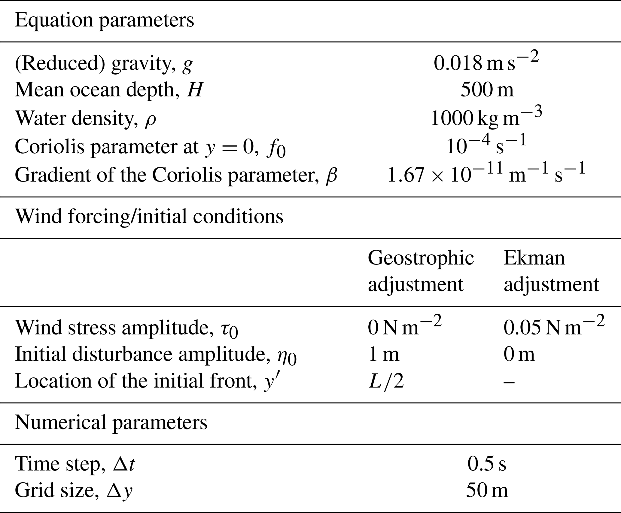
The domain is periodic in the zonal direction with walls parallel to the x-axis located at y=0 and y=L. The domain's meridional extent, L, was varied between L=4 to L=60 (in units of R_d) and is noted in each case. Since the differential system involves only variations in t and y (while x-variation is ignored), we set the number of cells in the x-direction to 4 to ensure the periodicity in x, so the zonal extent of the domain is 4Δx, where Δx is the grid spacing. No x variations were developed in the numerical simulations. The model parameters are summarized in Table 1. The Rossby radius of deformation, $R_{\mathrm{d}}=\sqrt{gH}/f_{\mathrm{0}}$, is set to 30 km – a typical value for the first baroclinic mode in the midlatitude ocean (Chelton et al., 1998). Note that the model parameters are given in dimensional form. However, the numerical results are presented in nondimensional form using the scales listed in Sect. 2.4.

Table 1 Model parameters. In addition to the parameters listed in the table, the Rossby radius of deformation, $R_{\mathrm{d}}=\sqrt{gH}/f_{\mathrm{0}}$, was set to 30  m throughout, and the domain's meridional extent, L, was varied between L=4R_d and L=60R_d (the value is always noted).

In the Ekman adjustment problem, we focus on the time-dependent velocity component $v^{\prime }(y,t)=v(y,t)-\stackrel{\mathrm{‾}}{v}\left(y\right)$. However, the modified MITgcm we constructed solves the RSWE, so the simulations include also the time-independent mean component, $\stackrel{\mathrm{‾}}{v}\left(y\right)$. This mean flow corresponds to the solution of the inhomogeneous part of the eigenvalue problem Eq. (12) i.e. Eq. (13). Therefore, when comparing the numerical simulations with the analytical wave solutions, we subtract $\stackrel{\mathrm{‾}}{v}$ from the total velocity v(y,t) in the simulations to isolate the time-dependent component v^′. The time-independent component $\stackrel{\mathrm{‾}}{v}\left(y\right)$ was obtained by solving Eq. (13) with scipy's solve_bvp function. To validate this procedure, we employed an alternative approach in which $\stackrel{\mathrm{‾}}{v}$ was computed by averaging v over many wave periods. As expected, the results from the direct numerical solution of Eq. (13) were indistinguishable from the long-term averages of v (see discussion and figures in Yacoby et al., 2024, in particular Sect. IV A 2 and Fig. 2). The solutions for $\stackrel{\mathrm{‾}}{v}$ are also used to calculate the coefficients of the eigenfunctions, $a_n^{*}$, in Eq. (26).

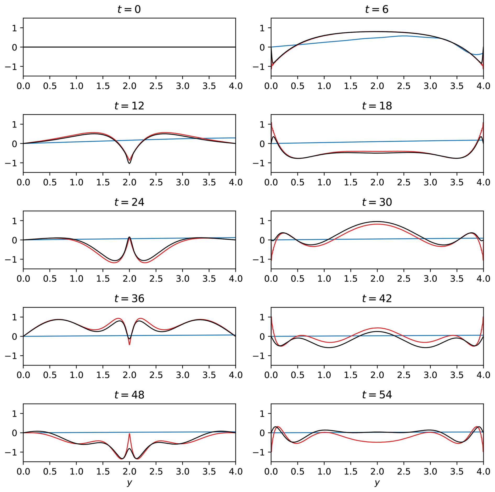
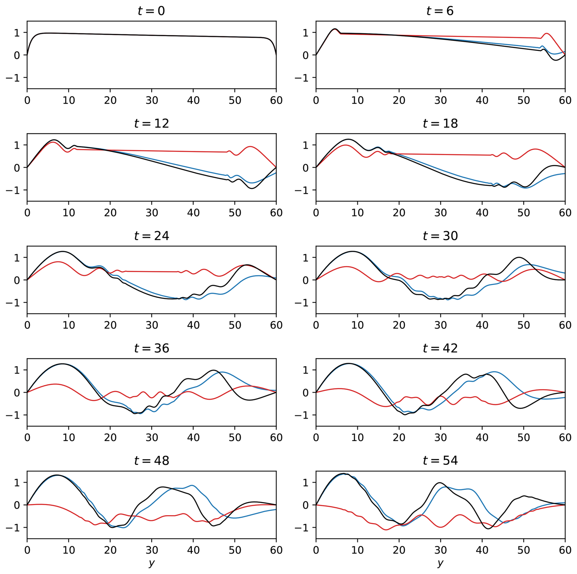
Figure 1 The meridional velocity, $v(y,t)=v^{\prime }$, in the geostrophic adjustment problem for L=4. Black lines: Numerical simulations; Red lines: Analytical harmonic waves; Blue lines: Analytical trapped waves. Time, t, is in units of $f_{\mathrm{0}}^{-\mathrm{1}}$.

In the calculation of the trapped wave solutions, the upper bound of the summation in Eqs. (18) and (25), i.e., the number of modes summed, was set to 10⁴. In contrast, summing such a large number of modes in the calculation of the harmonic wave solutions led to numerical errors. Therefore, for the harmonic solutions only, the number of summed modes was reduced to 500 (this issue is discussed in Sect. 5).

4.1 Results

The results in this section are presented in four figures, structured as follows. For each problem (the geostrophic adjustment and the Ekman adjustment) we display the solution of $v^{\prime }(y,t)=v(y,t)-\stackrel{\mathrm{‾}}{v}\left(y\right)$ for narrow (L=4) and wide (L=60) channels derived by subtracting the time-independent analytic solutions from the simulations. Each figure compares the simulated $v^{\prime }(y,t)$ (depicted by black lines) with the analytical solutions of v^′ derived for harmonic (red lines) and trapped (blue lines) waves. The figures show snapshots of v^′ at intervals of 6 time units. Although each of the 4 cases (2 problems and 2 channel widths) exhibits different leading frequencies, we chose to maintain intervals of 6 time units in all 4 figures so the results are presented in a uniform style of display.

Before presenting the results, it is worth noting that in fixed time snapshots, the differences between simulations and analytical solutions, as well as the differences between the two analytical solutions, can result from two reasons: The first is the disparities between the spatial structures (i.e. the eigenfunctions) of the harmonic, trapped, and simulated waves and the second is differences between the frequencies (i.e. the eigenvalues) of the harmonic, trapped, and simulated waves (since the difference might be smaller/larger at an earlier/later time). Both contributing factors should be considered in explanations of the differences between different cases.

Figure 2 As in Fig. 1 but for L=60.

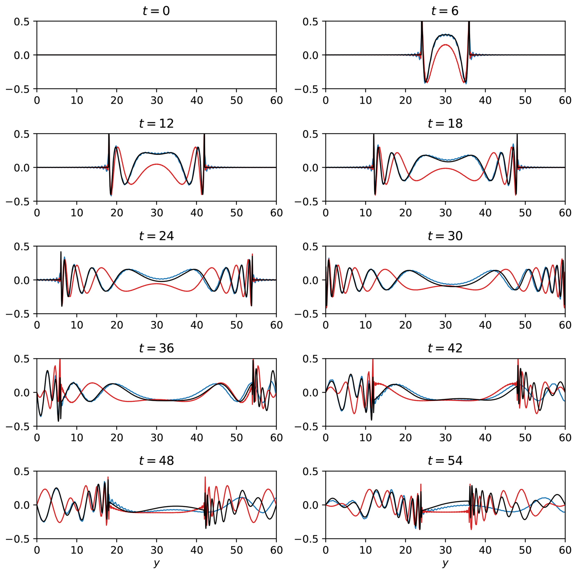
Figure 1 shows v^′ in the geostrophic adjustment problem for L=4. Note that the time in this figure, as well as in all other figures, is the nondimensional time that equals the dimensional time multiplied by f₀. The agreement between the harmonic wave solutions (red lines) and the numerical results (black lines) is acceptable up to t⪅40 while the trapped wave solutions (blue lines) are entirely irrelevant to the numerical results. Beyond t=40 the simulated waves deviate appreciably from the anticipated structure of harmonic waves. The discrepancy between the two is particularly noticeable in the center of the channel at t=42 and t=54. We hypothesize that this appreciable difference between the harmonic wave structures and the numerically simulated waves is due to a slight difference between the harmonic and numerical frequencies rather than differences in the harmonic and numerical meridional wave structures. In addition to the discrepancy between the harmonic and the numerical frequencies, we also observe a difference in the amplitudes of harmonic and simulated waves at the wave-fronts. The wave-fronts of harmonic waves are larger and sharper compared to those obtained from the simulations, which is particularly noticeable near the domain boundaries at t=18, 30, 42, and 54, and at the center of the domain at t=48. This difference between the theory and the simulations is likely due to the dissipation applied in the MITgcm that reduces the energy contained in the short wave limit. At lower resolutions of both y and t the gap between the theory and simulation at y=2 evident at t=48 occurs earlier and the gap at t=48 is larger by a factor of about 2.

Figure 2 shows v^′ in the geostrophic adjustment problem for L=60. The harmonic wave solutions (red lines) differ substantially from the numerical results (black lines), except near the wave-fronts. In contrast, there is a very good agreement between the trapped wave theory (blue lines) and the numerical results up to t=30. This agreement reaffirms the neglect of the y² terms in the derivation of the eigenvalue equation Eq. (15). At t=30, the wave-fronts reach the domain boundaries and are reflected towards the center of the domain. This reflection is observed in the numerical results and the harmonic wave solutions. However, in the trapped wave solutions, the waves are reflected only from the southern wall (at y=0). Consequently, a discrepancy between the trapped wave structure and that of the numerical results develops near the northern wall and propagates southward at the speed of the wave-fronts that equals 1 in non-dimensional units (i.e. $\sqrt{gH}$ in dimensional units, since $R_{\mathrm{d}}{f}_{\mathrm{0}}=\sqrt{gH}$). This is evident, for example, at t=48, at which time the northern wave-front, that had reached the northern wall at t=30, is located at $y=\mathrm{42}=\mathrm{60}-\mathrm{18}$. Thus, the trapped wave theory yields incorrect results between y=42 and y=60. Regardless of the reflection, a small, yet, noticeable difference can be observed between the trapped wave theory and the numerical results, particularly for t≥24 and near the center of the domain. We hypothesize that this difference arises from a slight difference between the trapped frequencies and the numerical frequencies.

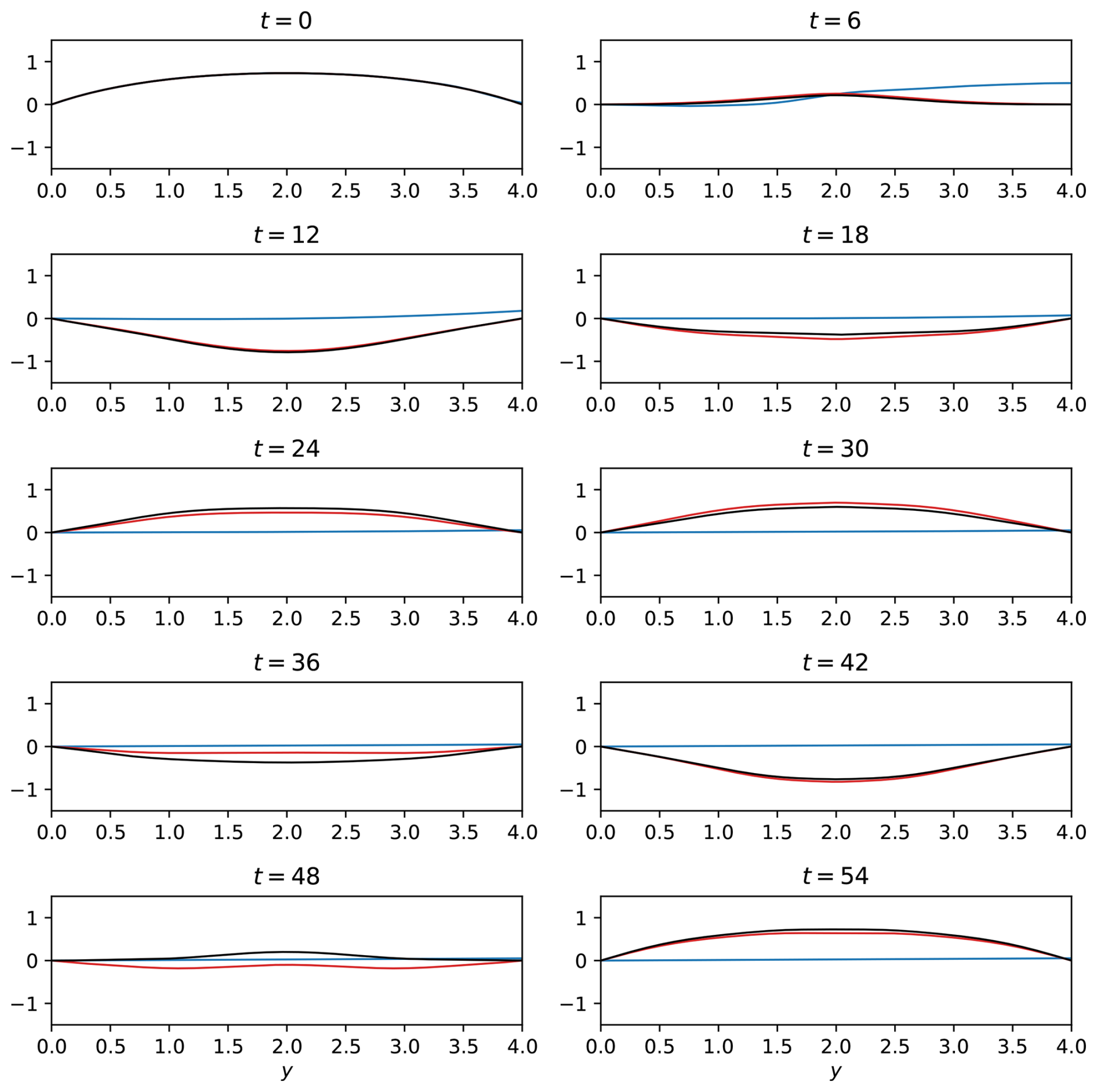
Figure 3 The time-dependent component of the meridional velocity, $v^{\prime }=v(y,t)-\stackrel{\mathrm{‾}}{v}\left(y\right)$, in the Ekman adjustment problem for L=4. Black lines: Numerical simulations; Red lines: Analytical harmonic waves; Blue lines: Analytical trapped waves. Time, t, is in units of $f_{\mathrm{0}}^{-\mathrm{1}}$.

Figure 3 shows v^′ in the Ekman adjustment problem for L=4. As in the geostrophic adjustment problem (Fig. 1), the agreement between the harmonic waves (red lines) and the simulations (black lines) is good, though, as in Fig. 1, a discrepancy is evident between the harmonic and numerical frequencies. In this case, the discrepancy is particularly noticeable at t=36 and t=48. As expected, the trapped wave structure (blue lines) is irrelevant to the simulations at L=4.

Figure 4 shows v^′ in the Ekman adjustment problem for L=60. As in the geostrophic adjustment problem (Fig. 2), the harmonic wave solutions (red lines) differ substantially from the numerical results (black lines). For t≤18, the discrepancy between the harmonic wave theory and the numerical results is more significant in the northern side of the domain than in its southern side. This may be related to the fact that the term −2by, which is ignored in the harmonic wave theory, increases linearly with y. The trapped wave theory (blue lines) matches the numerical results only for small t. As in the geostrophic adjustment problem, the mismatch between the theory and the simulations develops at the northern wall and spreads southwards. However, in the Ekman adjustment problem, this southward spread begins at t=0. Consequently, in the Ekman adjustment problem, the trapped wave theory provides reasonable results for shorter times compared to the geostrophic adjustment problem. For example, in the Ekman adjustment problem the trapped wave theory yields reasonable results at t=48 only for y<20 while in the geostrophic adjustment problem, it yields reasonable results for y<30.

Figure 4 As in Fig. 3 but for L=60.

4.2 Error estimates

The visual comparisons in Figs. 1–4 are useful but inherently qualitative. To complement them with a more systematic and reproducible metric, we introduce a quantitative diagnostic error measure, ϵ(t), defined as the spatially averaged absolute difference between the theoretical and numerical $v^{\prime }(y,t)$ fields:

$$\begin{array}{}\text{(27)}& \begin{array}{rl}\mathit{ϵ}\left(t\right)& ={\displaystyle \frac{\mathrm{1}}{\mathrm{600}}}\sum _{m=\mathrm{0}}^{\mathrm{600}}|v_{\mathrm{theory}}^{\prime }\left(t,y={\displaystyle \frac{mL}{\mathrm{600}}}\right)\\ & -v_{\mathrm{numerical}}^{\prime }\left(t,y={\displaystyle \frac{mL}{\mathrm{600}}}\right)|.\end{array}\end{array}$$

Here $v_{\mathrm{theory}}^{\prime }$ is evaluated either from the harmonic or the trapped wave solutions, and $v_{\mathrm{numerical}}^{\prime }$ from the MITgcm simulations. The purpose of ϵ(t) is not to introduce a new physical quantity, but to provide a simple and compact diagnostic that quantifies the agreement across different theories, problems, and channel widths.

Figure 5 shows the time dependence of ϵ(t). In all cases, ϵ(t) exhibits relatively fast oscillations. These arise because even a small frequency mismatch between theoretical and numerical solutions can lead to alternating phases of agreement and disagreement. To highlight the longer-term behavior, we applied a third-order low-pass Butterworth filter with a cutoff frequency of 0.05 (corresponding to $\mathrm{5}\times {\mathrm{10}}^{-\mathrm{6}}$ s⁻¹ in dimensional units). The filtered quantity, ϵ^LP(t), is shown as solid curves in Fig. 5. This filtering suppresses high-frequency variations while retaining the overall growth or decay trends.

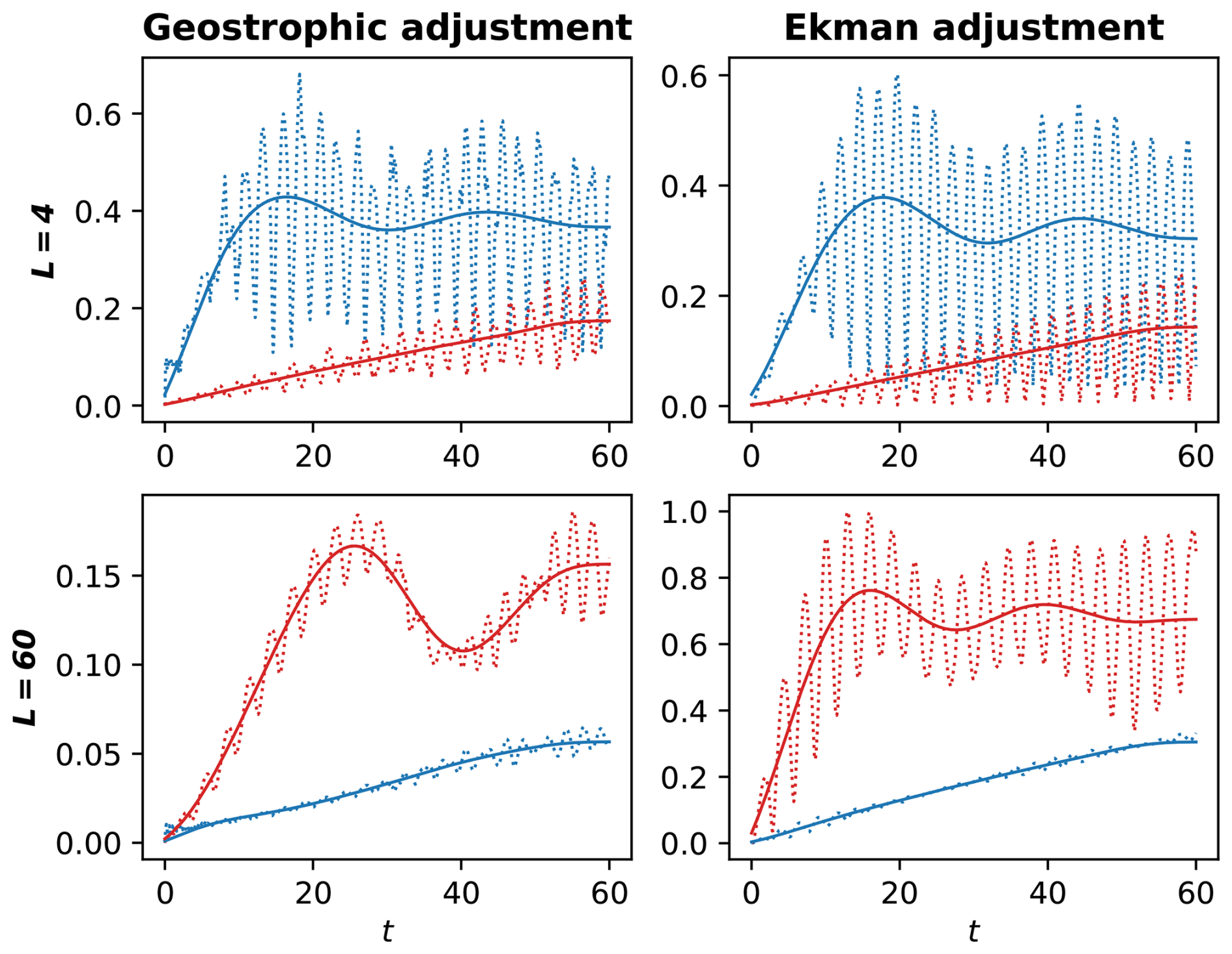
Figure 5 Temporal evolution of the errors. Dotted lines: the time-dependent difference between the wave theories and the numerical solutions, ϵ(t) defined in Eq. (27). Red dotted lines: harmonic wave theory. Blue dotted lines: trapped wave theory. Solid lines: low-pass filter of the corresponding dotted lines – ϵ^LP(t). Time, t, is in units of $f_{\mathrm{0}}^{-\mathrm{1}}$.

For L=4, the harmonic wave solutions are closer to the numerical solutions than the trapped wave solutions. In both the geostrophic adjustment problem (upper-left panel) and the Ekman adjustment problem (upper-right panel), ϵ^LP(t) shows similar magnitudes and trends. In the harmonic wave theory (red lines), ϵ^LP(t) increases linearly with time, while in the trapped wave theory (blue lines), it exhibits low-frequency oscillations that pass the low-pass filter.

For L=60, the trapped wave solutions are closer to the numerical solutions compared to the harmonic wave solutions. In both the geostrophic adjustment (lower-left panel) and the Ekman adjustment (lower-right panel) problems, ϵ^LP(t) shows similar trends. In the trapped wave theory (blue lines), ϵ^LP(t) increases linearly with time, while in the harmonic wave theory (red lines), it exhibits low-frequency oscillations. However, ϵ^LP(t) is approximately five times larger in the Ekman adjustment problem compared to the geostrophic adjustment problem in both harmonic- and trapped-wave theories.

In the last analysis of error employed here, ϵ(t) is computed for values of L that vary between L=4 to L=60 with intervals of 4 in the two problems and the two wave theories. The resulting low-pass filtered ϵ, ϵ^LP, are shown in Fig. 6 as a function of t and L. Clearly, the changes in ϵ^LP with t and L do not follow a uniform pattern. It is worth noting that the maximal error occurs in the harmonic wave solution for the Ekman adjustment problem (upper right panel). The variation of ϵ^LP in the trapped wave solution of the geostrophic adjustment problem (lower left panel) is monotonic in both t and L. In the Ekman adjustment problem the best agreement between the simulations and the trapped wave theory occurs near L=30. These results are further discussed in Sect. 5. We emphasize that ϵ(t) and its filtered counterpart are employed here strictly as diagnostic tools. Their purpose is to provide an objective and reproducible way of summarizing the complex spatio-temporal differences between theories and simulations, rather than to serve as physical novel quantities. Nevertheless, the systematic trends they reveal, such as the crossover between harmonic and trapped dominance with increasing L and the gradual increase in mismatch with time, help clarify the regimes of validity of each theory and the mechanisms by which they depart from the numerical solutions.

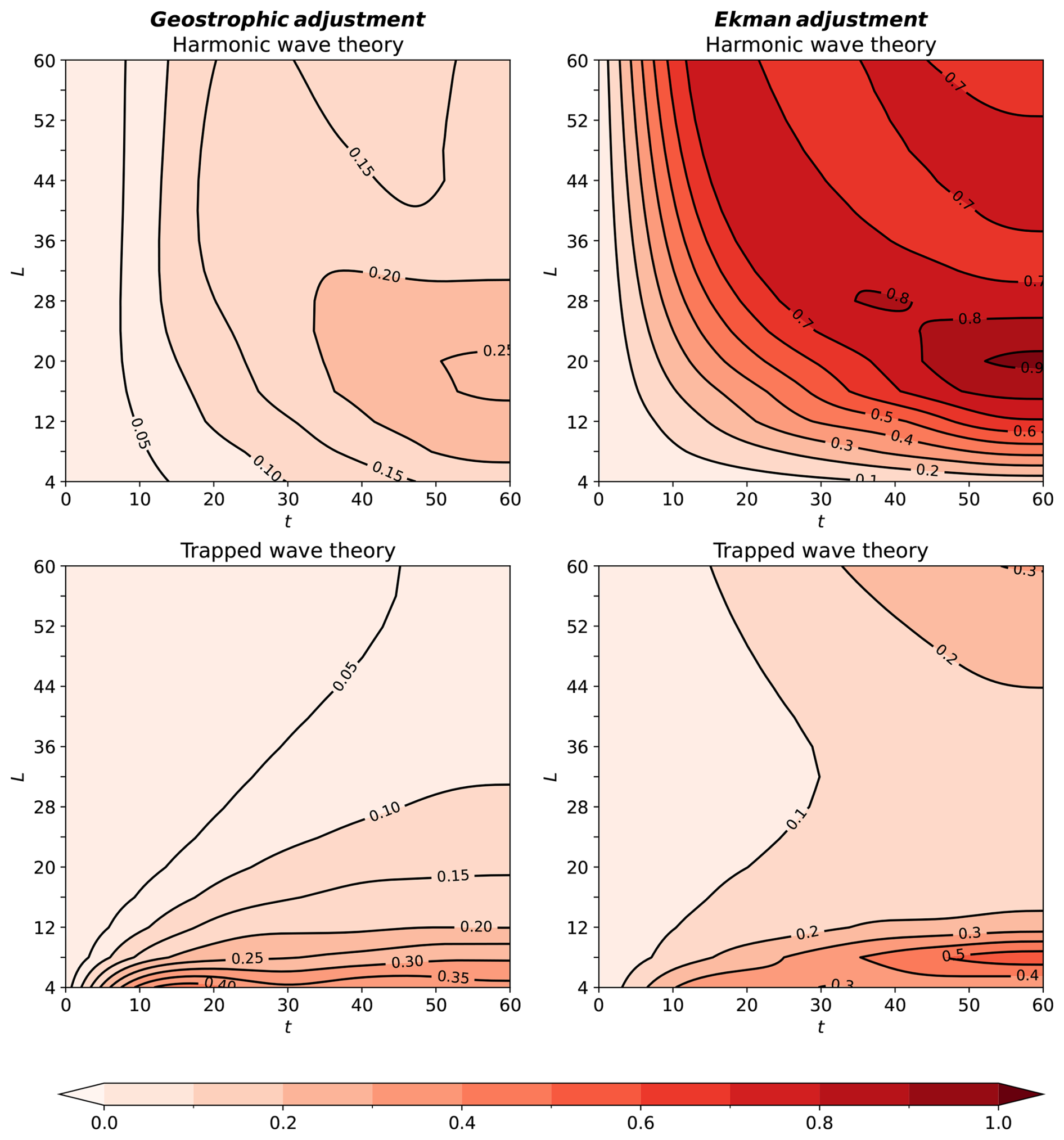
Figure 6 Contours of low-pass filtered ϵ, ϵ^LP, on the t and L plane in the two physical problems and for the two wave theories. Time, t, is in units of $f_{\mathrm{0}}^{-\mathrm{1}}$.

5 Summary and discussion

This work examined the applicability of two wave theories on the mid-latitude β-plane – the harmonic and the trapped wave theories – to the temporal evolution evidenced in numerical simulations. The examination is based on the derivation of one-dimensional, zonally-invariant, wave solutions for two physical problems – the geostrophic adjustment and the Ekman adjustment problems. The analytical solutions are then compared to numerical simulations conducted using the MITgcm. The numerical simulations are assumed to be accurate and the aim in comparing the theories with numerical simulations is to evaluate the applicability of the idealized theories, rather than the accuracy of the simulations.

The discrepancies between the two theories and numerical simulations were quantified using ϵ(t), defined in Eq. (27), focusing on its low-pass filtered, ϵ^LP(t). The discrepancies originate from different approximations associated with each theory. The harmonic wave theory, which neglects the β effect, becomes less accurate when the meridional domain, L, increases to L=20, with more complex variations beyond this domain size (upper panels of Fig. 6). On the other hand, the trapped wave solutions of the geostrophic adjustment problem, that account consistently for β, neglect the family of eigenfunctions associated with the second Airy function – Bi are more accurate as L increases as they better satisfy the boundary condition at the north wall with the increase in L (lower-left panel of Fig. 6). However, in the Ekman adjustment problem, optimal agreement occurs near L≈30 (lower-right panel of Fig. 6). Intuitively, the increase of ϵ^LP with L for L>30 can be attributed to the larger number of wave modes required to accurately describe the solution in large domains, while the number of wave modes used here was identical at all values L. To test this hypothesis, ϵ^LP in the Ekman adjustment problem was recalculated with the number of summed modes equal to 10³ and 5×10⁴ (whereas the number of modes used throughout was 10⁴). Contrary to intuition, the effect on ϵ^LP of the change in the number of summed wave modes was insignificant for small t and practically 0 for large t.

Our results clearly demonstrate the failure of the trapped wave theory in small domains. This failure is attributed to two reasons. The main reason, which plays a role in both problems, is that the Airy functions Ai(y) can not satisfy the boundary condition of $v^{\prime }=\mathrm{0}$ at y=L when L is small. The second reason for the failure is that the superposition of Ai(y) modes fails to satisfy the initial conditions of v. In both cases Bi(y) must be added to the solution in order to satisfy the boundary condition at y=L or the initial condition of v. This reason contributes to the failure of the trapped wave theory only in the geostrophic adjustment problem. The failure of the Ai(y) modes to satisfy the initial condition (Eq. 19) at small domains is demonstrated in Fig. 7 where $\frac{\partial v^{\prime }}{\partial t}(t=\mathrm{0})=\sum _{n=\mathrm{0}}^N{\mathit{\omega }}_n{a}_n^{*}{\widehat{v}}_n^{*}\left(y\right)$ is shown for the harmonic waves (red lines) and trapped waves (blue lines) for L=4 (left panel) and L=60 (right panel). As in Figs. 1–4, the number of summed-up modes, N, is set to  0 in the expansion to harmonic waves and to 10⁴ in the expansion to trapped waves. Except for the blue curve on the left panel, all curves accurately approximate $\partial v^{\prime }/\partial t(t=\mathrm{0})=\mathrm{2}\mathit{\delta }(y-y^{\prime })$ as is evident from the values of the integrals over the curves that should be 2.0 for a Dirac delta function. The calculated values of the integrals (indicated in the figure using red and blue legends) are close to 2. The largest deviation, of about 5 %, occurs for trapped waves in small domains which is evident in the blue curve (and associated legend) on left panel. In contrast to the geostrophic adjustment problem, in the Ekman adjustment problem, the superposition of Ai modes satisfies the initial condition (Eq. 24) even when L=4, as illustrated in the upper-left panel of Fig. 3.

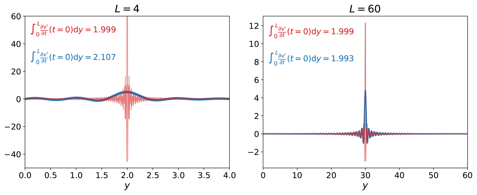
Figure 7 The derivative of v^′ with respect to t at t=0 in the geostrophic adjustment problem. Left panel: L=4. Right panel: L=60. Red lines: harmonic waves. Blue lines: trapped waves. The ordinate of the left panel is truncated at 60, though the maximal value of the red curve is 184, to ensure the finite values of both curves at y≠2 can be clearly seen. According to Eq. (19), the curves should satisfy $\partial v^{\prime }(t=\mathrm{0})/\partial t=\mathrm{2}\mathit{\delta }(y-y^{\prime })$ so the area under the curves should be 2.00. The areas under the red and blue curves are noted in the figure using red and blue legends, respectively.

In large domains, the harmonic theory does not reproduce several features of the simulations, primarily because of the omission of the β effect (recall: Rossby waves are filtered out by the k=0 assumption) rather than from the limited number of summed harmonic modes (500 compared to 10⁴ Airy modes). This conclusion is evident upon comparisons with the f-plane simulations, where the summation over 500 harmonic modes produces accurate results, confirming that the harmonic wave theory effectively describes the f-plane dynamics (results not shown). Errors in the harmonic solutions also stem from the inclusion of modes with tiny amplitudes in the summation, especially in the Ekman adjustment problem, where the superposition of harmonic modes fails to satisfy the initial condition for v^′, Eq. (24). These errors are less pronounced in the geostrophic adjustment problem but still affect the wave-front amplitudes. Nevertheless, it should be noted that the harmonic theory can be extended locally through WKBJ-type approximations, which account for the slow meridional variation of the Coriolis parameter by using a local dispersion relation. This local interpretation has been widely applied in geophysical contexts and provides additional validity to the harmonic framework beyond the strict global solutions considered here.

Although both problems share the same governing equation, Eq. (14), their forcing mechanisms are different. In the geostrophic adjustment problem waves are driven by localized initial perturbations and for small $t<L/\mathrm{2}$ the trapped wave theory agrees with the simulations. However, at larger t the neglect of the Bi functions causes discrepancies when the simulated waves are reflected from both walls while trapped waves are reflected from the south wall only. In contrast, in the Ekman adjustment problem, waves are driven by constant wind stress and violate the boundary conditions at y=L from the outset.

In both problems, the discrepancies between the theories and the simulations increase with time. However, for large values of L the error of the harmonic wave theory is larger in the Ekman adjustment problem than in the geostrophic adjustment problem (compare the ordinate ranges of the lower panels of Fig. 5). Part of the reason for the higher values of ϵ^LP(t) in the Ekman adjustment problems arises from the higher amplitude of the waves themselves in the Ekman adjustment problem compared to the geostrophic adjustment problem (compare the ordinate range of Fig. 2 to that of Fig. 4).

Figure 8 summarizes the ranges of L and t where the theories yield acceptable results, defined by ϵ^LP<0.1. The colors in Fig. 8 indicate which theory satisfies ϵ^LP<0.1 as a function of L and t using the following color codes: White: both theories. Red: harmonic wave theory. Blue: trapped wave theory. Black: neither theory. Regions in which neither theory is accurate are wider in the Ekman adjustment problem, reflecting the greater challenges of modeling its dynamics. In both problems, the trapped wave theory yields ϵ^LP<0.1 over larger ranges of L and t compared to the harmonic wave theory. As evident from the white regions near the ordinates of Fig. 8, both theories satisfy ϵ^LP<0.1 for sufficiently small t. This is because the superposition of harmonic and trapped wave modes in the two problems was selected such that the resulting functions satisfy the initial conditions. The failure of the trapped wave theory at large L in the Ekman adjustment problem does not result from the small number of modes, as a change in the number of modes (to 10³ and 5×10⁴) has a negligible effect on ϵ^LP. This delicate issue is left for future study.

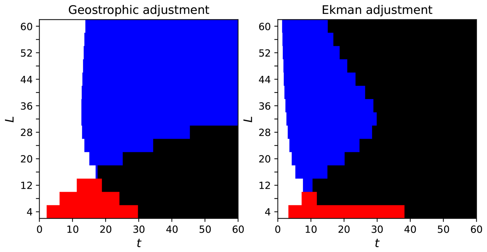
Figure 8 The range of L and t for which the harmonic and trapped wave theories yields ϵ^LP<0.1. White: both theories. Red: only the harmonic wave theory. Blue: only the trapped wave theory. Black: neither theory. Time, t, is in units of $f_{\mathrm{0}}^{-\mathrm{1}}$.

This study expands on earlier works by examining the accuracy of wave theories across both time and domain ranges (L-values), rather than focusing solely on two values of L (one small and one large) as was done in Gildor et al. (2016) and Yacoby et al. (2023). It demonstrates that neither of the existing wave theories provides accurate approximations for the waves at all (large) times. This underscores the need for a more comprehensive theory that incorporates the β effect while fully satisfying the boundary conditions. An approach to achieve this goal is to decompose the initial conditions into the basis of the two Airy functions, Ai and Bi, while satisfying the boundary conditions, based on solutions of the transcendental equations that currently have no known explicit solutions.

This paper focuses on zonally-invariant Poincaré waves. However, the approach employed here can also be applied to zonally-dependent problems, e.g., geostrophic adjustment in rotating channels (Gill, 1976; Hermann et al., 1989; Tomasson and Melville, 1992, Sect. 9, and Yacoby et al., 2023, Sect. 5), geostrophic adjustment in closed basins (Johnson and Grimshaw, 2014), and wind-driven circulation in closed basins (Pedlosky, 1965; Pierini, 1998; Sura et al., 2000; LaCasce, 2000; Cessi and Primeau, 2001; Cessi and Louazel, 2001). The extension of this work to a zonally-dependent setup, where Rossby waves are also excited, is left for future works.

Appendix A: Harmonic- and trapped-wave theories

This appendix reviews the two types of wave solutions of Eq. (15). We start with classical harmonic waves in Sect. A1 and proceed to trapped waves in Sect. A2. In addition to the solutions for v (that are the main focus of this work) we also provide, for completeness of presentation, the solutions for η and u in Appendix B.

A1 Harmonic waves

Although the classical harmonic wave theory is well-known, its discussion here serves to highlight the differences between this wave type and the trapped waves presented in Sect. A2.

In the harmonic theory, the y-dependent term −2by is neglected in Eq. (15). Considering the boundary conditions (Eq. 5), the resulting equation is solved by the harmonic eigenfunctions:

$$\begin{array}{}\text{(A1)}& {\widehat{v}}_n=a_n\sin \left[{\displaystyle \frac{\mathit{\pi }(n+\mathrm{1})}{L}}y\right],n=\mathrm{0},\mathrm{1},\mathrm{\dots }\end{array}$$

and the associated eigenvalues:

$$\begin{array}{}\text{(A2)}& E_n={\left({\displaystyle \frac{\mathit{\pi }(n+\mathrm{1})}{L}}\right)}^{\mathrm{2}},n=\mathrm{0},\mathrm{1},\mathrm{\dots }\end{array}$$

The coefficients a_n are determined in Sect. 3 based on the initial conditions. Substituting the expression for E_n in Eq. (17) yields the dispersion relation for harmonic Poincaré waves:

$$\begin{array}{}\text{(A3)}& {\mathit{\omega }}_n^{\mathrm{2}}=\mathrm{1}+{\left({\displaystyle \frac{\mathit{\pi }(n+\mathrm{1})}{L}}\right)}^{\mathrm{2}}.\end{array}$$

Before moving on to the trapped wave theory we define the normalized harmonic eigenfunctions:

$$\begin{array}{}\text{(A4)}& {\widehat{v}}_n^{*}\left(y\right)=\sqrt{{\displaystyle \frac{\mathrm{2}}{L}}}\sin \left[{\displaystyle \frac{\mathit{\pi }(n+\mathrm{1})}{L}}y\right],\end{array}$$

in which the coefficient $\sqrt{\frac{\mathrm{2}}{L}}$ guarantees that:

$$\begin{array}{}\text{(A5)}& \langle {\widehat{v}}_n^{*},{\widehat{v}}_n^{*}\rangle =\underset{\mathrm{0}}{\overset{L}{\int }}{\left({\widehat{v}}_n^{*}\left(y\right)\right)}^{\mathrm{2}}\mathrm{d}y=\mathrm{1}.\end{array}$$

The definition of ${\widehat{v}}_n^{*}$ is employed in Sect. 3 to determine the coefficient a_n in Eq. (A1).

Note that in the absence of zonal variations, the harmonic wave solutions are identical to those on the f-plane.

A2 Trapped waves

This section presents the trapped wave theory, in which the harmonic wave functions of Sect. A1 are replaced by Airy functions, as has been shown by Paldor and Sigalov (2008), De-Leon and Paldor (2011), Gildor et al. (2016), and Yacoby et al. (2023).

In the trapped wave theory, Eq. (15) is transformed to an Airy equation:

$$\begin{array}{}\text{(A6)}& {\displaystyle \frac{{\mathrm{d}}^{\mathrm{2}}\widehat{v}}{\mathrm{d}{z}^{\mathrm{2}}}}-z\widehat{v}=\mathrm{0}\end{array}$$

by defining

$$z\left(y\right)=-\left(\mathrm{2}b{)}^{-\mathrm{2}/\mathrm{3}}\right[E-\mathrm{2}by].$$

The general solution of Eq. (A6) is a linear combination of Ai(z), that decays (faster than exponential) for z>0, and Bi(z), that grows (faster than exponential) for z>0, namely:

$$\begin{array}{}\text{(A7)}& \widehat{v}=a\mathrm{Ai}\left(z\right)+b\mathrm{Bi}\left(z\right),\end{array}$$

where the coefficients a and b are determined from the initial and/or boundary conditions.

A2.1 Semi-infinite domains

In semi-infinite domains (L→∞), the boundary condition that v vanishes at infinity implies that the coefficient of Bi (that grows to infinity) in Eq. (A7) must be 0. Accordingly, using the definition of z(y), Eq. (A7) reduces to:

$$\begin{array}{}\text{(A8)}& \widehat{v}=a\mathrm{Ai}\left(-\left(\mathrm{2}b{)}^{-\mathrm{2}/\mathrm{3}}\right[E-\mathrm{2}by]\right).\end{array}$$

The final step is the application of the wall boundary condition at y=0, i.e. setting z(y=0) in the expression of the nth zero of Ai(z), denoted as ξ_n, e.g., ${\mathit{\xi }}_{\mathrm{0}}=-\mathrm{2.338}$, ${\mathit{\xi }}_{\mathrm{1}}=-\mathrm{4.088}$, etc. (note that ξ_n are all negative since Ai(z) vanishes only at finite negative values of z). This condition determines the discrete wave functions:

$$\begin{array}{}\text{(A9)}& {\widehat{v}}_n=a_n\mathrm{Ai}\left((\mathrm{2}b{)}^{\mathrm{1}/\mathrm{3}}y+{\mathit{\xi }}_n\right)\end{array}$$

with the corresponding eigenvalues:

$$\begin{array}{}\text{(A10)}& E_n=-{\mathit{\xi }}_n(\mathrm{2}b{)}^{\mathrm{2}/\mathrm{3}}.\end{array}$$

Substituting this expression for E_n in Eq. (16) yields the following dispersion relation for trapped Poincaré waves:

$$\begin{array}{}\text{(A11)}& {\mathit{\omega }}_n^{\mathrm{2}}=\mathrm{1}-{\mathit{\xi }}_n(\mathrm{2}b{)}^{\mathrm{2}/\mathrm{3}}.\end{array}$$

As in Sect. A1 we define the normalized (Airy) eigenfunctions:

$$\begin{array}{}\text{(A12)}& {\widehat{v}}_n^{*}\left(y\right)={\left[{\displaystyle \frac{{\mathrm{2}}^{\mathrm{2}/\mathrm{3}}}{\mathrm{2}{b}^{\mathrm{1}/\mathrm{3}}}}{\left({\mathrm{Ai}}^{\prime }\left({\mathit{\xi }}_n\right)\right)}^{\mathrm{2}}\right]}^{-\mathrm{1}/\mathrm{2}}\mathrm{Ai}\left((\mathrm{2}b{)}^{\mathrm{1}/\mathrm{3}}y+{\mathit{\xi }}_n\right),\end{array}$$

where Ai^′(z) is the derivative of Ai(z). The coefficient of Ai(z) in Eq. (A12) guarantees that:

$$\langle {\widehat{v}}_n^{*},{\widehat{v}}_n^{*}\rangle =\underset{\mathrm{0}}{\overset{\mathrm{\infty }}{\int }}{\left({\widehat{v}}_n^{*}\left(y\right)\right)}^{\mathrm{2}}\mathrm{d}y=\mathrm{1}.$$

Note that here the upper bound of the integral is ∞ [and not L as in Eq. (A5)] since the trapped wave modes, Ai(z), vanish at infinity. The form of ${\widehat{v}}_n^{*}$ given in Eq. (A12) is employed in Sect. 3 to determine the coefficient a_n in Eq. (A9).

A2.2 Large finite domains

Since all Airy wave solutions in Eq. (A9) decay to 0 at large y, these solutions can be expected to apply at sufficiently large, finite, y-domains and not only to semi-infinite domains. Indeed, Paldor and Sigalov (2008), Gildor et al. (2016), and Yacoby et al. (2023) demonstrate that the trapped wave theory provides an accurate approximation for the waves when the domain length, L, is large enough e.g. when:

$$\begin{array}{}\text{(A13)}& L>(\mathrm{2}b{)}^{-\frac{\mathrm{1}}{\mathrm{3}}}\left(\mathrm{2}+{\mathit{\xi }}_n\right)\end{array}$$

which guarantees that $z(y=L)>\mathrm{2}$ so $\mathrm{Ai}\left(z\right(y=L\left)\right)<\mathrm{0.035}$, which is sufficiently small to justify the neglect of Bi(z). The above constraint on L indicates that the higher the wave mode, n (and with it, the absolute value of ξ_n), the larger the domain should be for the trapped wave theory to remain valid. However, this condition completely ignores the time variable, which may also affect the applicability of the trapped wave theory in large but finite domains.

The condition (Eq. A13) points to the combined dependence of the β-effect on the domain extent L and R_d. Though the condition applies to the transition from the harmonic (i.e. the f-plane) wave solutions to the trapped (Airy) wave solutions, its implication is wider and the effect of β on the f-plane dynamics is determined by both L and R_d as was shown in Yacoby et al. (2024).

Appendix B: The solutions of η and u

For completeness of presentation, this Appendix provides the solutions for η and u. We start with the geostrophic adjustment problem in Sect. B1 and proceed to the Ekman adjustment problem in Sect. B2.

B1 Geostrophic adjustment

In the geostrophic adjustment problem, η and u can be divided into time-independent components ($\stackrel{\mathrm{‾}}{\mathit{\eta }}$, $\stackrel{\mathrm{‾}}{u}$) and time-dependent components (η^′, u^′).

B1.1 Time-independent components

According to Eq. (10), the time-independent components $\stackrel{\mathrm{‾}}{\mathit{\eta }}$ and $\stackrel{\mathrm{‾}}{u}$ satisfy the geostrophic balance:

$$\begin{array}{}\text{(B1)}& (\mathrm{1}+by)\stackrel{\mathrm{‾}}{u}=-{\displaystyle \frac{\partial \stackrel{\mathrm{‾}}{\mathit{\eta }}}{\partial y}}.\end{array}$$

However, an additional equation must be derived to find $\stackrel{\mathrm{‾}}{\mathit{\eta }}$ and $\stackrel{\mathrm{‾}}{u}$. The derivation of this additional equation outlined here follows the approach presented in Yacoby et al. (2023). Substituting the continuity equation, Eq. (11), into the y derivative of Eq. (9) yields:

$$\begin{array}{}\text{(B2)}& {\displaystyle \frac{\partial q}{\partial t}}=bv,q={\displaystyle \frac{\partial u}{\partial y}}+(\mathrm{1}+by)\mathit{\eta }.\end{array}$$

Substituting the continuity equation once again but this time into the y derivative of Eq. (B2), yields:

$$\begin{array}{}\text{(B3)}& {\displaystyle \frac{\partial }{\partial t}}\left({\displaystyle \frac{\partial q}{\partial y}}+b\mathit{\eta }\right)=\mathrm{0}.\end{array}$$

This conservation equation indicates that the combination of time-dependent variables within the bracket at time t equals their initial combination. The initial conditions (Eqs. 6–7) imply:

$$q(t=\mathrm{0})=-(\mathrm{1}+by)\mathrm{sgn}(y-y^{\prime }),$$

and substituting this relation into the time integral of Eq. (B3) yields:

$$\begin{array}{}\text{(B4)}& \begin{array}{rl}{\displaystyle \frac{{\partial }^{\mathrm{2}}u}{\partial y^{\mathrm{2}}}}& +(\mathrm{1}+by){\displaystyle \frac{\partial \mathit{\eta }}{\partial y}}+\mathrm{2}b\mathit{\eta }=-\mathrm{2}(\mathrm{1}+by)\mathit{\delta }(y-y^{\prime })\\ & -\mathrm{2}b\mathrm{sgn}(y-y^{\prime }).\end{array}\end{array}$$

The system (Eqs. B1 and B4) can be solved numerically by imposing the relevant boundary conditions (see discussion in Yacoby et al., 2023) and utilizing a standard BVP solver.

B1.2 Waves

After finding v^′, the wave components of u and η, u^′ and η^′, can be obtained by substituting v^′ into Eqs. (9) and (11), respectively, and integrating these equations with respect to time. This results in:

$$\begin{array}{}\text{(B5)}& u^{\prime }=-(\mathrm{1}+by)\sum _{n=\mathrm{0}}^{\mathrm{\infty }}{\displaystyle \frac{a_n^{*}}{{\mathit{\omega }}_n}}{\widehat{v}}_n^{*}\left(y\right)\cos \left({\mathit{\omega }}_{n}t\right)\end{array}$$

and

$$\begin{array}{}\text{(B6)}& {\mathit{\eta }}^{\prime }=\sum _{n=\mathrm{0}}^{\mathrm{\infty }}{\displaystyle \frac{a_n^{*}}{{\mathit{\omega }}_n}}{\displaystyle \frac{\mathrm{d}{\widehat{v}}_n^{*}}{\mathrm{d}y}}\cos \left({\mathit{\omega }}_{n}t\right)\end{array}$$

where:

$${\displaystyle \frac{\mathrm{d}{\widehat{v}}_n^{*}}{\mathrm{d}y}}={\displaystyle \frac{\mathit{\pi }(n+\mathrm{1})}{L}}\sqrt{{\displaystyle \frac{\mathrm{2}}{L}}}\cos \left[{\displaystyle \frac{\mathit{\pi }(n+\mathrm{1})}{L}}y\right],$$

according to the harmonic wave theory, and:

$${\displaystyle \frac{\mathrm{d}{\widehat{v}}_n^{*}}{\mathrm{d}y}}=(\mathrm{2}b{)}^{\mathrm{1}/\mathrm{3}}{\left[{\displaystyle \frac{{\mathrm{2}}^{\mathrm{2}/\mathrm{3}}}{\mathrm{2}{b}^{\mathrm{1}/\mathrm{3}}}}{\left({\mathrm{Ai}}^{\prime }\left({\mathit{\xi }}_n\right)\right)}^{\mathrm{2}}\right]}^{-\mathrm{1}/\mathrm{2}}{\mathrm{Ai}}^{\prime }\left((\mathrm{2}b{)}^{\mathrm{1}/\mathrm{3}}y+{\mathit{\xi }}_n\right),$$

according to the trapped wave theory.

B2 Ekman adjustment

The calculated solutions of $\stackrel{\mathrm{‾}}{v}$ and v^′ yield η and u as follows: the substitution of $v=\stackrel{\mathrm{‾}}{v}+v^{\prime }$ in Eq. (11) and integration with respect to t yields:

$$\begin{array}{}\text{(B7)}& \mathit{\eta }=\stackrel{\mathrm{‾}}{\mathit{\eta }}\cdot t+{\mathit{\eta }}^{\prime }\end{array}$$

where:

$$\begin{array}{}\text{(B8)}& \stackrel{\mathrm{‾}}{\mathit{\eta }}=-{\displaystyle \frac{\mathrm{d}\stackrel{\mathrm{‾}}{v}}{\mathrm{d}y}},{\mathit{\eta }}^{\prime }=-\sum _{n=\mathrm{0}}^{\mathrm{\infty }}{\displaystyle \frac{a_n^{*}}{{\mathit{\omega }}_n}}{\displaystyle \frac{\mathrm{d}{\widehat{v}}_n^{*}}{\mathrm{d}y}}\sin \left({\mathit{\omega }}_{n}t\right).\end{array}$$

Substituting $v=\stackrel{\mathrm{‾}}{v}+v^{\prime }$ in Eq. (9) yields:

$$\begin{array}{}\text{(B9)}& u=\stackrel{\mathrm{‾}}{u}\cdot t+u^{\prime }\end{array}$$

in which:

$$\begin{array}{}\text{(B10)}& \stackrel{\mathrm{‾}}{u}={\displaystyle \frac{\mathrm{1}}{\mathrm{1}+by}}{\displaystyle \frac{{\mathrm{d}}^{\mathrm{2}}\stackrel{\mathrm{‾}}{v}}{\mathrm{d}{y}^{\mathrm{2}}}},u^{\prime }=(\mathrm{1}+by)\sum _{n=\mathrm{0}}^{\mathrm{\infty }}{\displaystyle \frac{a_n^{*}}{{\mathit{\omega }}_n}}{\widehat{v}}_n^{*}\left(y\right)\sin \left({\mathit{\omega }}_{n}t\right).\end{array}$$

The $\stackrel{\mathrm{‾}}{u}\cdot t$ term solves the inhomogeneous part of Eq. (9), i.e.:

$$\stackrel{\mathrm{‾}}{u}-(\mathrm{1}+by)\stackrel{\mathrm{‾}}{v}=\mathrm{1},$$

which is equivalent to Eq. (13). The u^′ component solves the homogeneous part of Eq. (9), i.e.:

$${\displaystyle \frac{\partial u^{\prime }}{\partial t}}-(\mathrm{1}+by)v^{\prime }=\mathrm{0}.$$

Appendix C: Extension to a two-layer ocean

In this appendix, we consider the case of a two-layer ocean. This analytically tractable configuration provides the motivation for the continuously stratified case discussed in Appendix D. To this end, the zonally invariant, linearized RSWE (Eqs. 1–3) are extended to the two-layer system. For the top layer of mean depth H₁ (with variables denoted by the subscript 1), the governing equations are:

$$\begin{array}{}\text{(C1)}& {\displaystyle }& {\displaystyle \frac{\partial u_{\mathrm{1}}}{\partial t}}-f\left(y\right)v_{\mathrm{1}}={\displaystyle \frac{{\mathit{\tau }}_{\mathrm{0}}}{{\mathit{\rho }}_{\mathrm{1}}{H}_{\mathrm{1}}}},\text{(C2)}& {\displaystyle }& {\displaystyle \frac{\partial v_{\mathrm{1}}}{\partial t}}+f\left(y\right)u_{\mathrm{1}}=-g{\displaystyle \frac{\partial \mathit{\eta }}{\partial y}},\text{(C3)}& {\displaystyle }& {\displaystyle \frac{\partial h}{\partial t}}-H_{\mathrm{1}}{\displaystyle \frac{\partial v_{\mathrm{1}}}{\partial y}}=\mathrm{0},\end{array}$$

where f(y) is given in Eq. (4), η is the free surface displacement and h is the (upward) displacement of the interface that separates the two layers. The continuity equation (Eq. C3) assumes $\left|\frac{\partial \mathit{\eta }}{\partial t}\right|\ll \left|\frac{\partial h}{\partial t}\right|$, an assumption referred to as the rigid lid approximation. For the lower layer (variables denoted by the subscript 2), the equations are:

$$\begin{array}{}\text{(C4)}& {\displaystyle }& {\displaystyle \frac{\partial u_{\mathrm{2}}}{\partial t}}-f\left(y\right)v_{\mathrm{2}}=\mathrm{0},\text{(C5)}& {\displaystyle }& {\displaystyle \frac{\partial v_{\mathrm{2}}}{\partial t}}+f\left(y\right)u_{\mathrm{2}}=-g{\displaystyle \frac{\partial \mathit{\eta }}{\partial y}}-g^{\prime }{\displaystyle \frac{\partial h}{\partial y}},\text{(C6)}& {\displaystyle }& {\displaystyle \frac{\partial h}{\partial t}}+H_{\mathrm{2}}{\displaystyle \frac{\partial v_{\mathrm{2}}}{\partial y}}=\mathrm{0},\end{array}$$

where H₂ is the mean thickness of the lower layer and $g^{\prime }=g({\mathit{\rho }}_{\mathrm{2}}-{\mathit{\rho }}_{\mathrm{1}})/{\mathit{\rho }}_{\mathrm{2}}$ (where ρ₁ and ρ₂ are the densities of the upper and lower layers, respectively) is the reduced gravity. The momentum equations (Eqs. C4–C5) assume $({\mathit{\rho }}_{\mathrm{2}}-{\mathit{\rho }}_{\mathrm{1}})/{\mathit{\rho }}_{\mathrm{2}}\ll \mathrm{1}$ while $g\frac{{\mathit{\rho }}_{\mathrm{2}}-{\mathit{\rho }}_{\mathrm{1}}}{{\mathit{\rho }}_{\mathrm{2}}}$ is O(1), an assumption referred to as the Boussinesq approximation. A more detailed derivation of Eqs. (C1)–(C6) can be found in Sect. 9.10 of Gill (1982).

The momentum equations can be combined to eliminate η from the equations, which is achieved by subtracting Eqs. (C1)–(C2) from Eqs. (C4)–(C5), respectively. The resulting equations are:

$$\begin{array}{}\text{(C7)}& {\displaystyle }& {\displaystyle \frac{\partial U_{\text{2-1}}}{\partial t}}-f\left(y\right)V_{\text{2-1}}=-{\displaystyle \frac{{\mathit{\tau }}_{\mathrm{0}}}{{\mathit{\rho }}_{\mathrm{1}}{H}_{\mathrm{1}}}},\text{(C8)}& {\displaystyle }& {\displaystyle \frac{\partial V_{\text{2-1}}}{\partial t}}+f\left(y\right)U_{\text{2-1}}=-g^{\prime }{\displaystyle \frac{\partial h}{\partial y}},,\end{array}$$

where:

$$U_{\text{2-1}}=u_{\mathrm{2}}-u_{\mathrm{1}},V_{\text{2-1}}=v_{\mathrm{2}}-v_{\mathrm{1}}.$$

A continuity equation that involves V_2-1 (instead of v₁ or v₂) is obtained by adding $H_{\mathrm{1}}^{-\mathrm{1}}$ times Eq. (C3) and $H_{\mathrm{2}}^{-\mathrm{1}}$ times Eq. (C6), which yields:

$$\left({\displaystyle \frac{\mathrm{1}}{H_{\mathrm{1}}}}+{\displaystyle \frac{\mathrm{1}}{H_{\mathrm{2}}}}\right){\displaystyle \frac{\partial h}{\partial t}}+{\displaystyle \frac{\partial V_{\text{2-1}}}{\partial y}}=\mathrm{0},$$

or:

$$\begin{array}{}\text{(C9)}& {\displaystyle \frac{\partial h}{\partial t}}+H_e{\displaystyle \frac{\partial V_{\text{2-1}}}{\partial y}}=\mathrm{0},\end{array}$$

where

$$H_e={\displaystyle \frac{H_{\mathrm{1}}{H}_{\mathrm{2}}}{H_{\mathrm{1}}+H_{\mathrm{2}}}}.$$

The two-layer system (Eqs. C7–C9) is similar to the single layer system (Eqs. 1–3) with two notable differences: (i) the RHS of Eq. (C7) contains a negative sign, whereas the RHS of Eq. (1) does not. (ii) The two-layer system includes two mean heights, H₁ and H₂ (or H₁ and H_e), whereas the one-layer system includes only one (H). In other words, the two-layer system introduces an additional free parameter.

C1 Nondimensionalization

As in Sect. 2.4, the two-layer system, Eqs. (C7)–(C9), is nondimensionalized (nondimensional variables are denoted by asterisks) by scaling the dimensional variables on:

$$\begin{array}{ll}{\displaystyle }& {\displaystyle }{t}^{*}=f_{\mathrm{0}}t,\\ {\displaystyle }& {\displaystyle }\left(x^{*},y^{*}\right)={\displaystyle \frac{\mathrm{1}}{R_{\mathrm{d}}^{\prime }}}(x,y),R_{\mathrm{d}}^{\prime }=\sqrt{g^{\prime }{H}_e}/f_{\mathrm{0}}.\end{array}$$

For the geostrophic adjustment problem (where τ₀=0), we also define:

$$\begin{array}{ll}{\displaystyle }& {\displaystyle }{h}^{*}={\displaystyle \frac{\mathrm{1}}{h_{\mathrm{0}}}}h,\\ {\displaystyle }& {\displaystyle }\left(U_{\text{2-1}}^{*},V_{\text{2-1}}^{*}\right)={\displaystyle \frac{H_e}{h_{\mathrm{0}}}}{\displaystyle \frac{\mathrm{1}}{\sqrt{g^{\prime }{H}_e}}}\left(U_{\text{2-1}},V_{\text{2-1}}\right),\end{array}$$

where h₀ is the amplitude of the initial interface disturbance (defined in Sect. D2), while, for the Ekman adjustment problem (where h₀=0) we define:

$$\begin{array}{ll}{\displaystyle }& {\displaystyle }{h}^{*}={\displaystyle \frac{H_{\mathrm{1}}}{H_e}}{\displaystyle \frac{{\mathit{\rho }}_{\mathrm{1}}{f}_{\mathrm{0}}\sqrt{g^{\prime }{H}_{\mathrm{1}}}}{{\mathit{\tau }}_{\mathrm{0}}}}h,\\ {\displaystyle }& {\displaystyle }\left(U_{\text{2-1}}^{*},V_{\text{2-1}}^{*}\right)={\displaystyle \frac{{\mathit{\rho }}_{\mathrm{1}}{f}_{\mathrm{0}}{H}_{\mathrm{1}}}{{\mathit{\tau }}_{\mathrm{0}}}}\left(U_{\text{2-1}},V_{\text{2-1}}\right).\end{array}$$

With these nondimensional variables, Eqs. (C7)–(C9) become:

$$\begin{array}{}\text{(C10)}& {\displaystyle }& {\displaystyle \frac{\partial U_{\text{2-1}}^{*}}{\partial t^{*}}}-(\mathrm{1}+b^{\prime }{y}^{*})V_{\text{2-1}}^{*}=-{\mathit{\delta }}_{i\mathrm{0}},\text{(C11)}& {\displaystyle }& {\displaystyle \frac{\partial V_{\text{2-1}}^{*}}{\partial t^{*}}}+\left(\mathrm{1}+b^{\prime }{y}^{*}\right)U_{\text{2-1}}^{*}=-{\displaystyle \frac{\partial h^{*}}{\partial y^{*}}},\text{(C12)}& {\displaystyle }& {\displaystyle \frac{\partial h^{*}}{\partial t^{*}}}+{\displaystyle \frac{\partial V_{\text{2-1}}^{*}}{\partial y^{*}}}=\mathrm{0},\end{array}$$

where:

$$b^{\prime }={\displaystyle \frac{\mathit{\beta }{R}_{\mathrm{d}}^{\prime }}{f_{\mathrm{0}}}}.$$

Note that although the dimensional two-layer system contains more parameters than the dimensional one-layer system, our somewhat cumbersome scaling (compared to that employed in Sect. 2.4) guarantees that the non-dimensional two-layer system contains only one free parameter, exactly as the non-dimensional single layer system.

Appendix D: Application to simulations with a 3D-OGCM

In this appendix, we extend the analytical insights from Appendix C to realistic simulations using the MITgcm, now employed as a fully 3-dimensional Ocean General Circulation Model, thereby demonstrating the relevance of our results to the real ocean.

Although the MITgcm is not inherently a layered model, we configure it with 38 vertical layers to represent a simplified, two-layer physical ocean. The upper and lower physical layers correspond to groups of numerical layers: the lower physical layer is initialized at temperature T₁, and the upper layer at T₂ (see Sect. D2). Section D2 provides a detailed description of how the numerical layers map onto the physical layers, clarifying that the “physical layers” serve as a conceptual framework for comparison with the two-layer analytical model of Appendix C, while the numerical layers determine the vertical resolution of the 3D-OGCM. Unlike the analytical model, which assumes a sharp interface preventing mixing, the 3D-OGCM includes temperature diffusion, allowing some mixing near the interface (i.e., within the thermocline).

D1 Equations solved

The MITgcm is employed here to simulate depth-dependent flow with density determined only by temperature. Viscous and diffusive terms are incorporated into the momentum equations and the temperature advection equation, respectively. Similar to the set-up in Sect. 2, the domain is periodic in the zonal direction and bounded in the meridional direction by walls located at y=0 and y=L and aligned parallel to the x-axis. A wind-stress momentum forcing is applied in the zonal momentum equation. However, in this multilayer configuration, the forcing term F_wind is applied only to the momentum equation for the surface layer, i.e., it is set to zero for the interior layers. While the MITgcm model equations account for x-variations, the initial conditions employed here (see Sect. D2) and the periodic boundary conditions in the x-direction ensure that no x-variation develops in the simulations (which was verified by our numerical simulations). Thus, although the equations of the MITgcm include the changes with x, the relevant equations in our problems assume $\partial /\partial x=\mathrm{0}$. These considerations lead to the following set of equations, written in Cartesian coordinates:

1. Momentum equations:

   $$\begin{array}{}\text{(D1)}& {\displaystyle }& {\displaystyle \frac{\mathrm{D}u(t,y,z)}{\mathrm{D}t}}-f\left(y\right)v-A_y{\displaystyle \frac{{\partial }^{\mathrm{2}}u}{\partial y^{\mathrm{2}}}}-A_z{\displaystyle \frac{{\partial }^{\mathrm{2}}u}{\partial z^{\mathrm{2}}}}=F_{\mathrm{wind}},\text{(D2)}& {\displaystyle }& {\displaystyle \frac{\mathrm{D}v(t,y,z)}{\mathrm{D}t}}+f\left(y\right)u-A_y{\displaystyle \frac{{\partial }^{\mathrm{2}}v}{\partial y^{\mathrm{2}}}}-A_z{\displaystyle \frac{{\partial }^{\mathrm{2}}v}{\partial z^{\mathrm{2}}}}=-{\displaystyle \frac{\mathrm{1}}{{\mathit{\rho }}_{\mathrm{0}}}}{\displaystyle \frac{\partial p^{\prime }}{\partial y}},\end{array}$$

   where

   $${\displaystyle \frac{\mathrm{D}}{\mathrm{D}t}}={\displaystyle \frac{\partial }{\partial t}}+v{\displaystyle \frac{\partial }{\partial y}}$$

   and $F_{\mathrm{wind}}=\frac{{\mathit{\tau }}_{\mathrm{0}}}{{\mathit{\rho }}_{\mathrm{0}}\mathrm{\Delta }{z}_s}$ is applied only to the momentum equation for the topmost layer. Here, A_y and A_z are horizontal and vertical viscosities, respectively, p is the pressure and ρ₀ is the mean water density (or the reference density in the equation of state, Eq. D5) and Δz_s is the thickness of the model's topmost layer.

2. Conservation of mass:

   $$\begin{array}{}\text{(D3)}& {\displaystyle \frac{\partial \mathit{\eta }(t,y)}{\partial t}}+{\displaystyle \frac{\partial V}{\partial y}}=\mathrm{0},\end{array}$$

   where η is the deviation of the sea surface height from z=0 and $V=\int v\mathrm{d}z$ (i.e. V is the vertically integrated meridional velocity in units of m² s⁻¹).

3. Equation for the perturbation pressure, p^′:

   $$\begin{array}{}\text{(D4)}& p^{\prime }(t,y,z)=g{\mathit{\rho }}_{\mathrm{0}}\mathit{\eta }+\underset{z}{\overset{\mathrm{0}}{\int }}g{\mathit{\rho }}^{\prime }\mathrm{d}z\end{array}$$

   separated into a barotropic part (due to variations in η) and a baroclinic part (due to variations in density anomaly, ρ^′).

4. Linear equation of state:

   $$\begin{array}{}\text{(D5)}& {\mathit{\rho }}^{\prime }(t,y,z)=\mathit{\rho }-{\mathit{\rho }}_{\mathrm{0}}=-{\mathit{\rho }}_{\mathrm{0}}\mathit{\alpha }\left(T-T_{\mathrm{0}}\right)\end{array}$$

   where α is the thermal expansion coefficient and T₀ is a reference temperature that determines ρ₀.

5. An advection-diffusion equation for the temperature, T:

   $$\begin{array}{}\text{(D6)}& {\displaystyle \frac{\mathrm{D}T(t,y,z)}{\mathrm{D}t}}-{\mathit{\kappa }}_y{\displaystyle \frac{{\partial }^{\mathrm{2}}T}{\partial y^{\mathrm{2}}}}-{\mathit{\kappa }}_z{\displaystyle \frac{{\partial }^{\mathrm{2}}T}{\partial z^{\mathrm{2}}}}=\mathrm{0}\end{array}$$

where κ_y and κ_z are horizontal and vertical diffusivities, respectively. The initial conditions and model parameters are described in Sect. D2.

D2 Initial conditions and model parameters

As in the one-layer case discussed in the main text (Sect. 2.3), we consider two types of initial conditions: one for the geostrophic adjustment problem and another for the Ekman adjustment problem. In both problems the ocean is initially at rest, its surface height, η, is zero and it consists of two layers of different temperatures (hence, different densities). The upper (lower) layer has a temperature of T₁ (T₂) with T₂<T₁ and a mean height of H₁ (H₂).

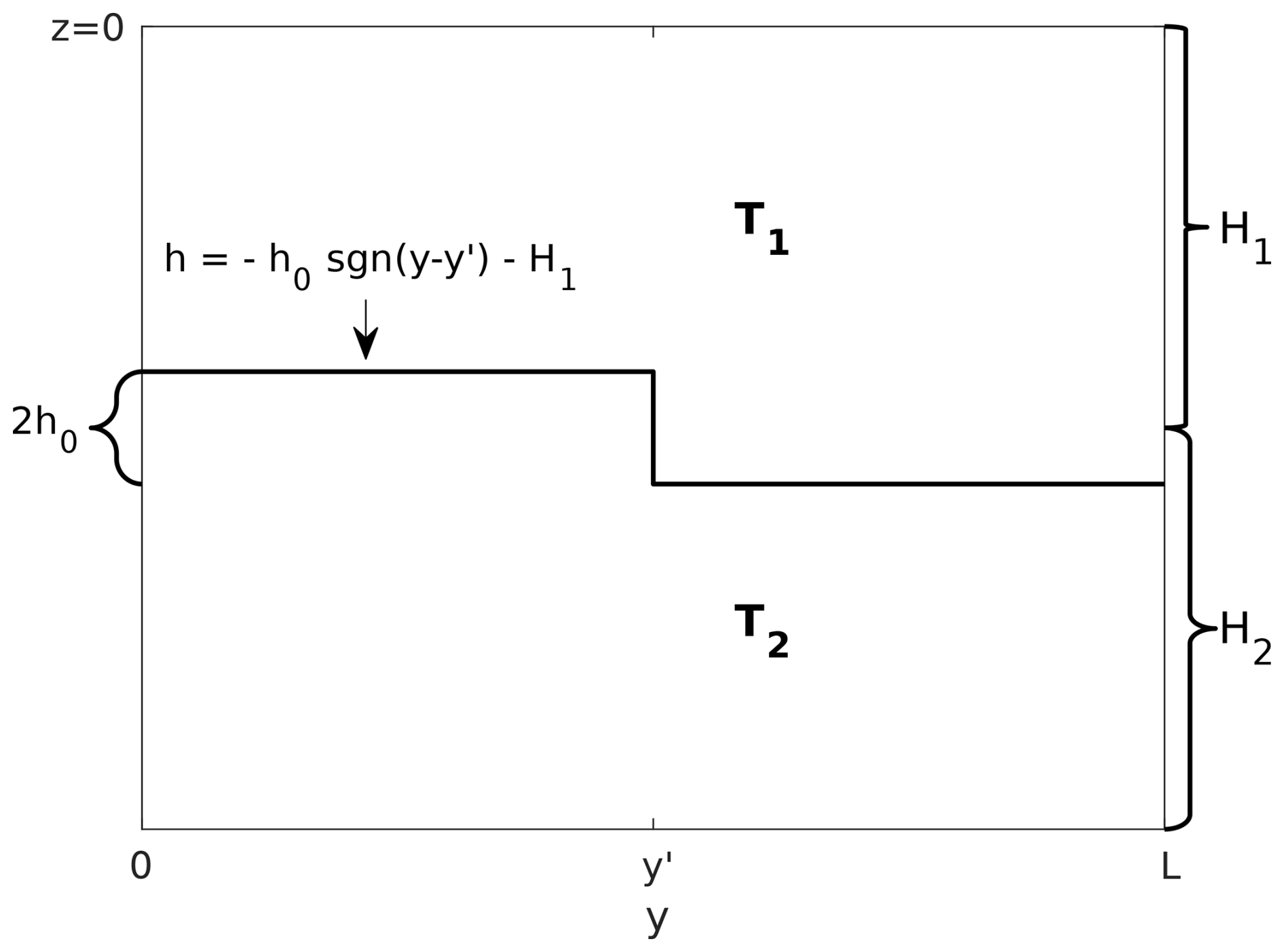
In the geostrophic adjustment problem, the forcing term on the RHS of Eq. (D1) is set to zero and the initial interface between the upper and lower layer, h(y,0) is given by:

$$h(y,t=\mathrm{0})=-h_{\mathrm{0}}\mathrm{sgn}(y-y^{\prime })-H_{\mathrm{1}},$$

where h₀ is the amplitude of the initial interface displacement. Accordingly, as illustrated in Fig. D1, the initial temperature field is:

$$\begin{array}{}\text{(D7)}& {\displaystyle }& {\displaystyle }T\left(y<y^{\prime },z,t=\mathrm{0}\right)=\left\{\begin{array}{cl}{T}_{\mathrm{1}},& \mathrm{for}-H_{\mathrm{1}}+h_{\mathrm{0}}<z\le \mathrm{0},\\ T_{\mathrm{2}},& \mathrm{otherwise},\end{array}\right.\text{(D8)}& {\displaystyle }& {\displaystyle }T\left(y>y^{\prime },z,t=\mathrm{0}\right)=\left\{\begin{array}{cl}{T}_{\mathrm{1}},& \mathrm{for}-H_{\mathrm{1}}-h_{\mathrm{0}}<z\le \mathrm{0},\\ T_{\mathrm{2}},& \mathrm{otherwise}.\end{array}\right.\end{array}$$

while the corresponding initial density anomaly (ρ^′) field, determined only by the temperature according to the linear equation of state Eq. (D5), is

$$\begin{array}{}\text{(D9)}& {\displaystyle }\begin{array}{rl}{\mathit{\rho }}^{\prime }& \left(y<y^{\prime },z,t=\mathrm{0}\right)\\ & =\left\{\begin{array}{cl}-{\mathit{\rho }}_{\mathrm{0}}\mathit{\alpha }\left(T_{\mathrm{1}}-T_{\mathrm{0}}\right),& \mathrm{for}-H_{\mathrm{1}}+h_{\mathrm{0}}<z\le \mathrm{0},\\ -{\mathit{\rho }}_{\mathrm{0}}\mathit{\alpha }\left(T_{\mathrm{2}}-T_{\mathrm{0}}\right),& \mathrm{otherwise},\end{array}\right.\end{array}\text{(D10)}& {\displaystyle }\begin{array}{rl}{\mathit{\rho }}^{\prime }& \left(y>y^{\prime },z,t=\mathrm{0}\right)\\ & =\left\{\begin{array}{cl}-{\mathit{\rho }}_{\mathrm{0}}\mathit{\alpha }\left(T_{\mathrm{1}}-T_{\mathrm{0}}\right),& \mathrm{for}-H_{\mathrm{1}}-h_{\mathrm{0}}<z\le \mathrm{0},\\ -{\mathit{\rho }}_{\mathrm{0}}\mathit{\alpha }\left(T_{\mathrm{2}}-T_{\mathrm{0}}\right),& \mathrm{otherwise}.\end{array}\right.\end{array}\end{array}$$

Figure D1 A schematic illustration of the initial temperature profile in the geostrophic adjustment problem (Eqs. D7–D8).

In the Ekman adjustment problem, the initial surface height disturbance, h₀, is set to zero, i.e.:

$$h(t=\mathrm{0})=-H_{\mathrm{1}}.$$

Thus, the corresponding initial temperature field is simply:

$$T(z,t=\mathrm{0})=\left\{\begin{array}{cl}{T}_{\mathrm{1}},& \mathrm{for}-H_{\mathrm{1}}<z\le \mathrm{0},\\ T_{\mathrm{2}},& \mathrm{otherwise}.\end{array}\right.$$

To avoid confusion between the number of layers in the ocean and the number of vertical grid cells in the model, we clarify that, although the initial conditions represent a two-layered ocean, the number of vertical grid cells in the numerical model (which will be termed here “numerical layers” to distinguish them from the two “physical” ocean layers) is set to 38. Specifically, in the Ekman adjustment problem, the upper 19 numerical layers were initialized with temperature T₁ (and anomaly density ${\mathit{\rho }}_{\mathrm{1}}^{\prime }$), whereas the lower 19 numerical layers were initialized with temperature T₂ (and anomaly density ${\mathit{\rho }}_{\mathrm{2}}^{\prime }$). In contrast, in the geostrophic adjustment problem, the number of numerical layers for the upper and lower layers were varied for $y<y^{\prime }$ and $y>y^{\prime }$ to represent an initial disturbance in the thermocline depth. Specifically, for $y>y^{\prime }$, the upper (physical) layer consists of 23 numerical layers, whereas for $y<y^{\prime }$, it consists of only 15 numerical layers.

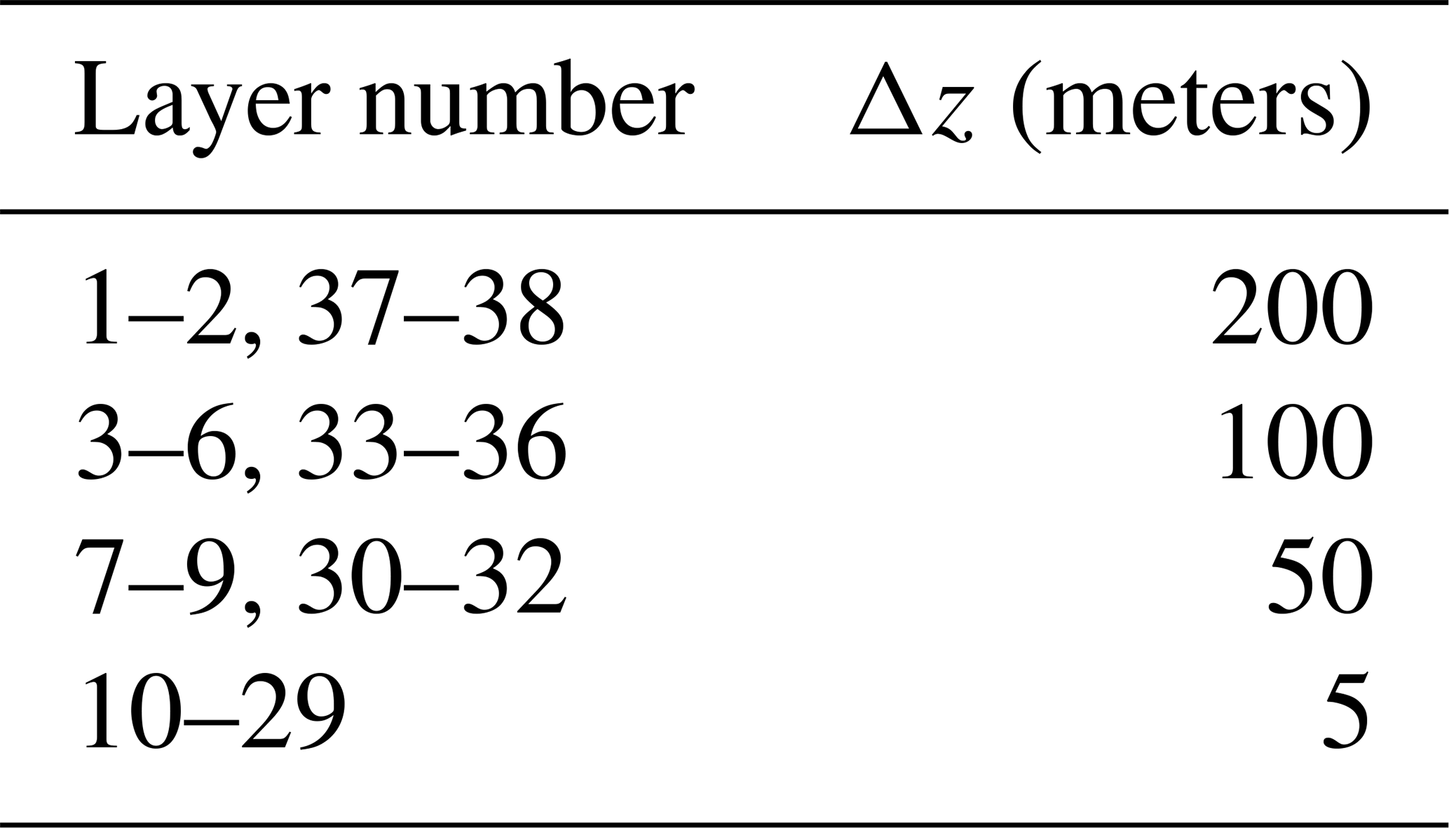
As detailed in Table D1, the grid size in the z-direction, Δz, in the 2 km deep ocean is not uniform, as a much finer resolution is required near the interface that separates the two layers (located 1 km below the surface). According to Table D1, a difference of 8 numerical layers in the thermocline represents a disturbance of 40 m in the depth of the thermocline.

Table D1 Vertical resolution, Δz. The model numerical layers are numbered from the sea surface (layer #1) to the ocean bottom (layer #38), with a total ocean depth of 2 km. Δz is finer near the interface between the layers, located at $z=-\mathrm{1}$ km (see Table D2).

The model parameters are summarized in Table D2. Note that

$$\begin{array}{ll}{\displaystyle }{H}_e& {\displaystyle }={\displaystyle \frac{H_{\mathrm{1}}{H}_{\mathrm{2}}}{H_{\mathrm{1}}+H_{\mathrm{2}}}}=\mathrm{500}\mathrm{m}\mathrm{and}{g}^{\prime }=g{\displaystyle \frac{{\mathit{\rho }}_{\mathrm{2}}-{\mathit{\rho }}_{\mathrm{1}}}{{\mathit{\rho }}_{\mathrm{2}}}}\\ {\displaystyle }& {\displaystyle }=g{\displaystyle \frac{\mathit{\alpha }\left(T_{\mathrm{1}}-T_{\mathrm{2}}\right)}{\mathrm{1}-\mathit{\alpha }\left(T_{\mathrm{2}}-T_{\mathrm{0}}\right)}}=\mathrm{0.018},\end{array}$$

which implies $R_{\mathrm{d}}^{\prime }=\sqrt{g^{\prime }{H}_e}/f_{\mathrm{0}}=\mathrm{30}$ km. This value is consistent with the value of R_d used in the 1D solutions presented in Sect. 4. This consistency ensures that the results of the current simulations can be directly compared with the previous results (see Sect. D3). The domain's meridional extent was set to L=1800 km $=\mathrm{60}{R}_{\mathrm{d}}^{\prime }$. Since x-variations are ignored in the differential system, we set the number of cells in the x-direction to 4 to ensure the periodicity in x (so the zonal extent of the domain is 4Δx, where Δx is the grid spacing). To ensure that the signs on the RHS of Eqs. (C7) and (1) agree with one another we set τ₀ in the current simulations to be negative (i.e., the wind blows from east to west).

Table D2 The parameters used for the 3D-OGCM. In addition to the parameters listed in the table, the Rossby radius of deformation, $R_{\mathrm{d}}^{\prime }=\sqrt{g^{\prime }{H}_e}/f_{\mathrm{0}}$, was set to 30 km, and the domain's meridional extent, L, is set to $\mathrm{60}{R}_{\mathrm{d}}^{\prime }$.

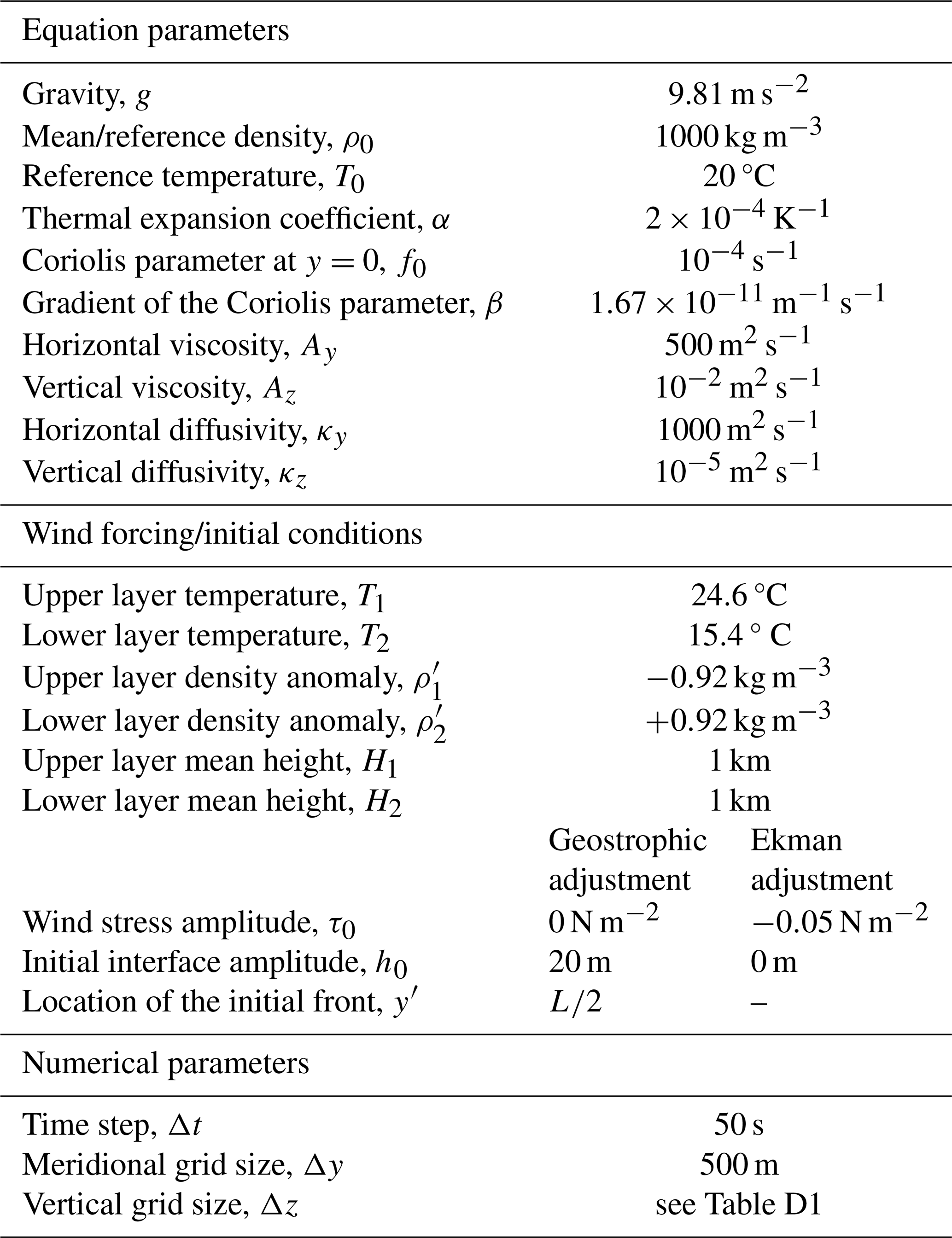
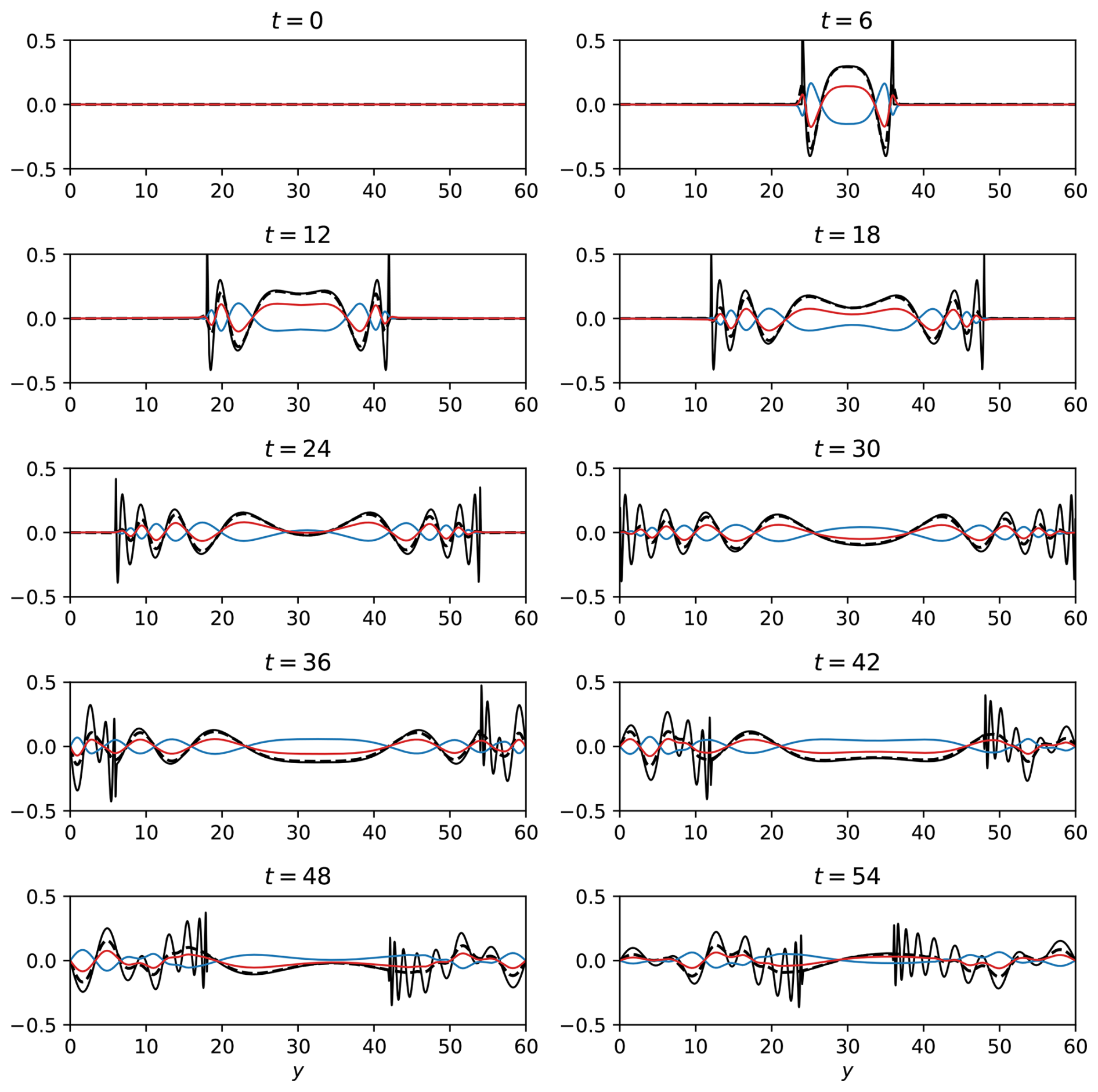
Figure D2 The meridional velocity for the geostrophic adjustment problem in multilayered ocean simulations. Red: the vertically averaged velocity of the lower layer, v₂. Blue: the vertically averaged velocity of the upper layer, v₁. Dashed-black: $V_{\text{2-1}}=v_{\mathrm{2}}-v_{\mathrm{1}}$. Solid-black: the meridional velocity in one-layer ocean simulations, v (duplicates of the solid-black lines shown in Fig. 2). Time, t, is in units of $f_{\mathrm{0}}^{-\mathrm{1}}$.

D3 Results

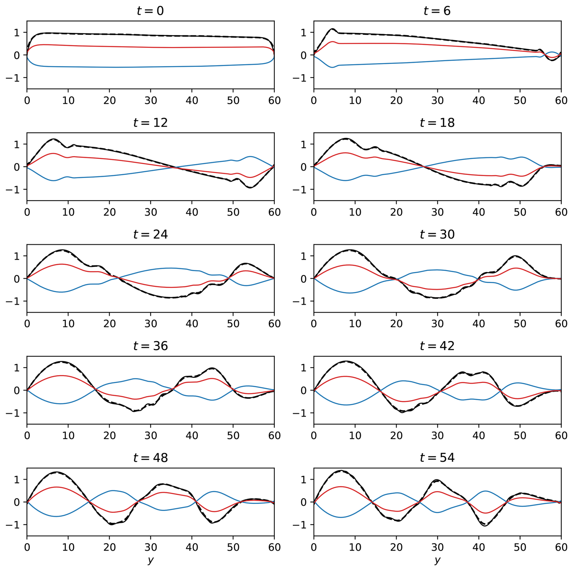
Figure D3 The time-dependent component of the meridional velocity for the Ekman adjustment problem in multilayered ocean simulations. Red: the vertically averaged velocity of the lower layer, $v_{\mathrm{2}}^{\prime }$. Blue: the vertically averaged velocity of the upper layer, $v_{\mathrm{1}}^{\prime }$. Dashed-black: $V_{\text{2-1}}^{\prime }=v_{\mathrm{2}}^{\prime }-v_{\mathrm{1}}^{\prime }$. Solid-black: the time-dependent component of the meridional velocity in one-layer ocean simulations, v^′ (duplicates of the solid-black lines shown in Fig. 4). Time, t, is in units of $f_{\mathrm{0}}^{-\mathrm{1}}$.

To compare the results of the current, multilayered ocean, simulations with the previous simulations of a single-layer ocean, we calculate the vertically-averaged meridional velocities in each of the two (physical) layers, i.e.:

$$v_{\mathrm{1}}={\displaystyle \frac{\mathrm{1}}{H_{\mathrm{1}}}}\underset{-H_{\mathrm{1}}}{\overset{\mathrm{0}}{\int }}v\mathrm{d}z,v_{\mathrm{2}}={\displaystyle \frac{\mathrm{1}}{H_{\mathrm{2}}}}\underset{-\left(H_{\mathrm{1}}+H_{\mathrm{2}}\right)}{\overset{H_{\mathrm{1}}}{\int }}v\mathrm{d}z,$$

where v₁ and v₂ are the vertically-averaged meridional velocities of the upper and lower layers, respectively. Since the model comprises 38 numerical layers, v₁ (v₂) is numerically computed as the average of the meridional velocities in the upper (lower) 19 layers. To focus on the waves, we subtract the time averages of v₁ and v₂ from their time-dependent values (v₁ and v₂) i.e., we calculate:

$$v_{\mathrm{1}}^{\prime }=v_{\mathrm{1}}-{\stackrel{\mathrm{‾}}{v}}_{\mathrm{1}},v_{\mathrm{2}}^{\prime }=v_{\mathrm{2}}-{\stackrel{\mathrm{‾}}{v}}_{\mathrm{2}},$$

where:

$$\begin{array}{ll}{\displaystyle }& {\displaystyle }{\stackrel{\mathrm{‾}}{v}}_{\mathrm{1}}={\displaystyle \frac{\mathrm{1}}{t_{\mathrm{end}}}}\underset{\mathrm{0}}{\overset{t_{\mathrm{end}}}{\int }}{v}_{\mathrm{1}}\mathrm{d}t,{\stackrel{\mathrm{‾}}{v}}_{\mathrm{2}}={\displaystyle \frac{\mathrm{1}}{t_{\mathrm{end}}}}\underset{\mathrm{0}}{\overset{t_{\mathrm{end}}}{\int }}{v}_{\mathrm{2}}\mathrm{d}t,\\ {\displaystyle }& {\displaystyle }{t}_{\mathrm{end}}=\mathrm{60}\left(\mathrm{in}\mathrm{units}\mathrm{of}{f}_{\mathrm{0}}^{-\mathrm{1}}\right).\end{array}$$

For the geostrophic adjustment problem we get ${\stackrel{\mathrm{‾}}{v}}_{\mathrm{1}}=\mathrm{0}={\stackrel{\mathrm{‾}}{v}}_{\mathrm{2}}$ which implies $v_{\mathrm{1}}=v_{\mathrm{1}}^{\prime }$ and $v_{\mathrm{2}}=v_{\mathrm{2}}^{\prime }$.

The results for the geostrophic adjustment and the Ekman adjustment problems are depicted in Figs. D2 and D3, respectively. In the figures, $v_{\mathrm{2}}^{\prime }$ is represented in red, $v_{\mathrm{1}}^{\prime }$ in blue, and the difference between them, $V_{\text{2-1}}^{\prime }=v_{\mathrm{2}}^{\prime }-v_{\mathrm{1}}^{\prime }$, in dashed-black lines. For comparison with the 1D simulations, the solid-black lines in Figs. D2 and D3 duplicates of the solid-black lines shown in Figs. 2 and 4, respectively. To allow a comparison between previous and current results, the results in Figs. D2 and D3 are presented in nondimensional form (using the scales described in Sect. C1).

The figures show excellent agreement between $V_{\text{2-1}}^{\prime }$ in the multilayered ocean simulations (dashed black) and v^′ in the simple single-layer ocean simulations (solid black) in both problems. However, in the geostrophic adjustment problem (Fig. D2), discrepancies between $V_{\text{2-1}}^{\prime }$ and v^′ are observed near the wave-fronts, where waves with a relatively short wavelength exist. We hypothesize two reasons for the discrepancies between $V_{\text{2-1}}^{\prime }$ and v^′: (i) the horizontal viscosity terms added to the momentum equations in the 3D-OGCM, Eqs. (D1)–(D2), reduce the energy of short waves in the multilayered ocean, resulting in smoother wave-fronts. (ii) To accelerate the multilayered ocean simulations, we significantly increased Δt and Δy in the 3D-OGCM (compare Table D2 with Table 1). As mentioned in Sect. 4.1, the sharpness of the wave-fronts decreases as Δt and Δy increase. In addition to the agreement between the single layer and multilayered simulations, the figures clearly indicate that in both problems $v_{\mathrm{1}}^{\prime }=-v_{\mathrm{2}}^{\prime }$ so $V_{\text{2-1}}^{\prime }=\mathrm{2}{v}_{\mathrm{2}}^{\prime }=-\mathrm{2}{v}_{\mathrm{1}}^{\prime }$.

We conclude this section with results not shown in the figures: (i) in both problems, the velocity in the lower layer is uniform with depth. Thus, the velocity at any depth below the interface equals the vertically averaged velocity of the lower layer, $v_{\mathrm{2}}^{\prime }$. (ii) In the geostrophic adjustment problem, the velocity in the upper layer is uniform with depth, as is the velocity in the lower layer. (iii) In the Ekman adjustment problem, the wind stress (which acts only at the topmost layer) causes a shear flow in the upper layer. We found that the profile of v^′(z) in the upper layer depends on the thickness of the model's topmost layer, Δz_s. However, the vertically averaged velocity $v_{\mathrm{1}}^{\prime }$ is independent of Δz_s since in a thinner grid layer the effect of the wind stress in that layer increases (the same wind stress is spread over a thinner layer).

Appendix E: Relevance to observations

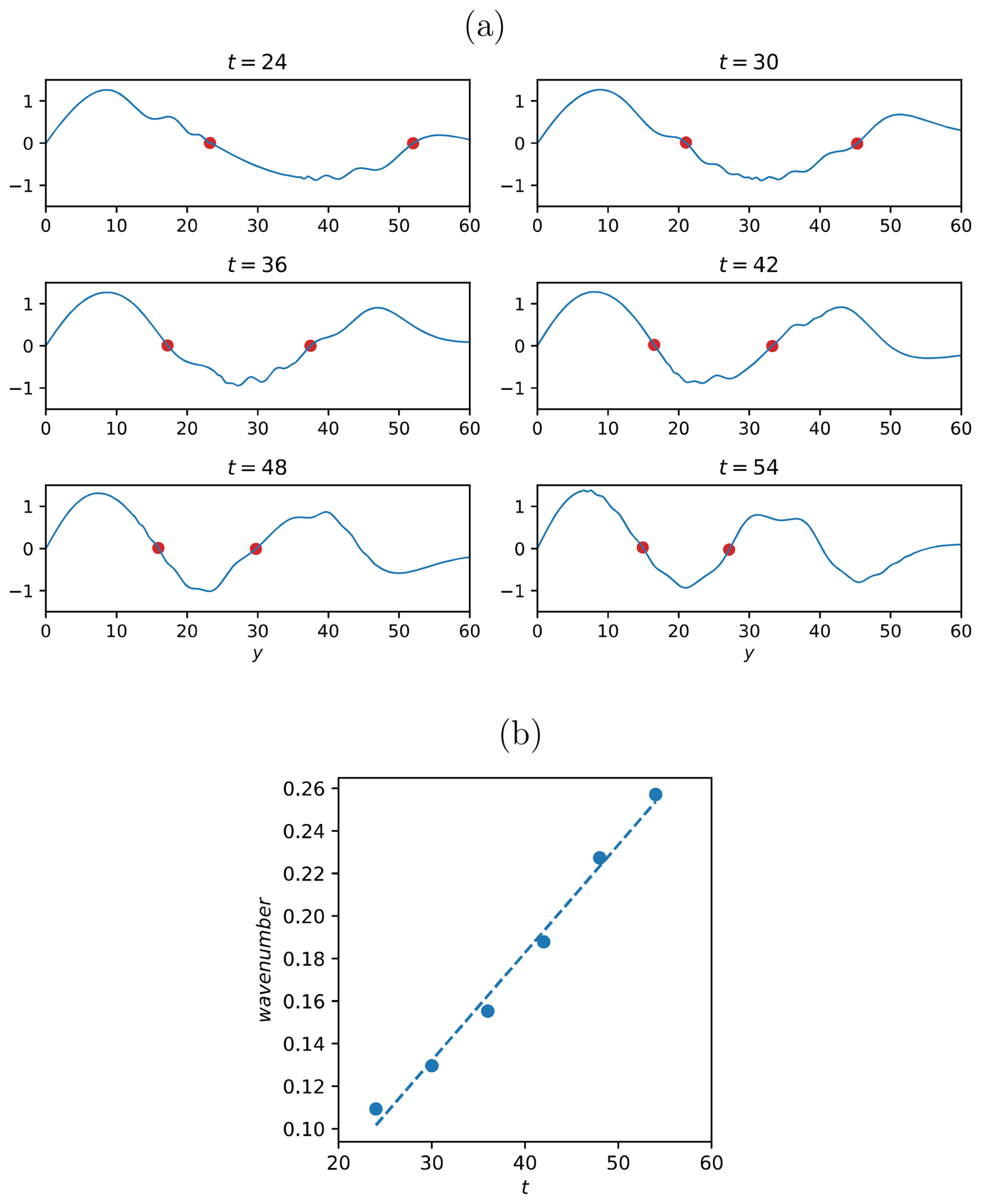
Figure E1 The decrease of the meridional wavelength with t (where t is given in units of $f_{\mathrm{0}}^{-\mathrm{1}}$). (a) The blue curves replicate the blue curves of Fig. 4, i.e., the trapped wave solutions in the Ekman adjustment problem at the indicated times, t. The red dots mark the two southern nodal points. The distance between the two red dots, D, is used in panel (b) to estimate the meridional wave number, $l\approx \mathit{\pi }/D$. (b) Dots: the estimated zonal wavenumber $\mathit{\pi }/D$ as a function of time. Dashed line: a linear regression fit. The slope of the regression line is $\mathrm{0.0051}\approx \mathit{\beta }{R}_{\mathrm{d}}/f_{\mathrm{0}}=\mathrm{0.005}$ which agrees very well with the observed trend reported by D'Asaro et al. (1995). The intersection with the ordinate is −0.02, indicating that the initial wavelength is 314. A 180° phase shift occurs at t=4.

Due to their relatively fast phase speed, Poincaré waves in the ocean are harder to observe compared to Rossby waves. Yet, reports of Poincaré wave observations were documented in the literature and they have been compared with analytical solutions and numerical simulations. For example, internal Poincaré waves were observed in Lake Ontario following a storm on 9 August 1972. Simons (1978) analyzed these observations and showed that both analytical and numerical solutions in idealized setting exhibit similar characteristics to the observed wave-fronts, e.g., the offshore propagation speed and the periodic recurrence with near-inertial periods. Simons (1978) also showed that the basic kinematics of the downwelling front could be simulated using a simple two-layer model.

Observations of the fast Poincaré waves require long and high-resolution in time and, similarly, the distinction between the mode structure of trapped and harmonic waves requires high meridional resolution and large meridional extent, both of which complicate the detection of these waves in the ocean. Presently, observations of Poincaré waves were reported mainly in lakes, where only harmonic modes can be detected, e.g., Lake Michigan and Lake Ontario (Mortimer, 1977). Indeed, Gill (1982, Sect. 7.3) cites these observations, emphasizing that the observed Poincaré waves have similar characteristics to the analytical harmonic-wave solutions of the geostrophic adjustment on the f-plane. Our results imply that the resemblance between both numerical and analytical solutions on the f-plane and the observed waves in Lake Ontario is expected, given that the meridional (south-north) extent of Lake Ontario is ∼80 km, which should be considered narrow since the results of Figs. 1 and 3 imply that a meridional extent of O(4) radii of deformation is narrow.

Poincaré waves with frequency near the inertial frequency f, known as near-inertial waves, are a dominant mode of high-frequency variability in the ocean, appearing as a prominent peak that rises significantly above the Garrett and Munk (1975) continuum internal wave spectrum (Alford et al., 2016). These waves are frequently observed in oceans and lakes, such as in the Gulf of Mexico (Gough et al., 2016), Lake Ontario (Schwab, 1977), Lake Michigan (Ahmed et al., 2014), the Gulf of Lions (Millot and Crépon, 1981), and the northeast Pacific Ocean (D'Asaro et al., 1995). The distinction between near-inertial trapped and harmonic modes of these near-inertial waves is complicated by the fact that the frequencies of the n=0 modes are very close to 1, hence to one another. This can be shown by substituting n=0 in Eq. (A3) which yields ${\mathit{\omega }}^{\mathrm{2}}=\mathrm{1}+(\mathit{\pi }/L{)}^{\mathrm{2}}$ for the harmonic n=0 mode while substituting n=0 (i.e., ${\mathit{\xi }}_{\mathrm{0}}=-\mathrm{2.338}$) and b=0.005 in Eq. (A11) yields ω²=1.1 for the trapped wave theory. For L=10 the two types of n=0 modes yield identical frequencies and for a larger/smaller value of L the frequency of the harmonic mode is only slightly smaller/larger than that of the trapped mode.

However, the trapped wave solution can be invoked to reproduce an observed phenomenon in the ocean – the linear change of the meridional wavenumber with time. The observations in the Pacific Ocean reported in D'Asaro et al. (1995) demonstrate that following a storm the zonal wavenumber remains constant while the meridional wavenumber changes linearly with time. Specifically, the meridional wavenumber decreases at a rate of −βt by, first, decreasing the initial wavenumber to zero followed by a 180° phase shift in which the wavenumber becomes negative and increases its absolute value linearly with time (see also Alford et al., 2016). This phenomenon was explained by D'Asaro et al. (1995) using the following argument: Representing an inertial wave on the β-plane (where $f=f_{\mathrm{0}}+\mathit{\beta }y$) as $e^{i(l_{\mathrm{0}}y-ft)}=e^{i\left[\right(l_{\mathrm{0}}-\mathit{\beta }t)y-f_{\mathrm{0}}t]}$ suggests that the initial meridional wavenumber l₀ becomes increasingly negative as βt increases. However, this heuristic argument is mathematically inconsistent since the ansatz $e^{i(l_{\mathrm{0}}y-f(y\left)t\right)}$ violates the separation of variable that yields the wave equation for the meridional structure (and the dispersion relation). Indeed, the harmonic wave solutions (red lines in Figs. 1–4) do not reproduce the linear time variation of the meridional wavenumber.

In contrast to the harmonic wave solutions, the trapped wave theory accurately reproduces the linear change of the wavenumber. To illustrate this, Fig. E1a revisits the trapped wave solutions for the Ekman adjustment problem shown in Fig. 4. The two southern nodal points are highlighted with red dots and the distance between these points, D, provides an estimate of the meridional wavenumber – $l\approx \mathit{\pi }/D$. As shown in Fig. E1b, the calculated wavenumber increases linearly with time. A linear regression analysis yields a slope of 0.0051, which is in excellent agreement with the theoretical value $\mathit{\beta }{R}_{\mathrm{d}}/f_{\mathrm{0}}=\mathrm{0.005}$ and the trend observed by D'Asaro et al. (1995).

The application of the theoretical results reported here to observations does not include the meridional structure of the modes and the wave's spectrum, since under typical conditions these properties cannot be deciphered in observations. However, laboratory experiments on a rotating table, similar to those reported in Cohen et al. (2010, 2012), can be carried out to verify the applicability of the theoretical results to carefully designed laboratory experiments.