Merging of a mesoscale eddy into the Lofoten Vortex in the Norwegian Sea captured by an ocean glider and SWOT observations

The Lofoten Vortex (LV) is an intense, apparently permanent anticyclone in the Lofoten Basin of the Norwegian Sea. It is characterised by a 1200 m thick core of Atlantic Water, with a radius of 15–20 km, in nearly solid-body rotation, reaching speeds up to 0.8 m s⁻¹. Potential vorticity in the core is nearly 2 orders of magnitude lower than the surroundings, creating a barrier to lateral mixing. It has previously been postulated that anticyclonic eddies in the Lofoten Basin, shed from the eastern branch of the Norwegian Atlantic Current along the Lofoten Escarpment, merge into the LV, contributing to maintaining its large heat and salt content and energetics, but such merging events have proven to be difficult to observe directly due to their transient and unpredictable nature. In April 2023, an eddy merger event was successfully observed using a combination of in situ data from an autonomous ocean glider and absolute dynamic topography (and derived velocities) from the fast sampling calibration phase of the Surface Water Ocean Topography (SWOT) satellite altimeter. During the observed merging process, an incoming eddy gradually approaches the LV and then elongates as the two begin to co-rotate and then merge, with a corresponding spin-up of vorticity and eddy kinetic energy and possible ejection of water of low potential vorticity from the merged LV core. The incoming eddy had a smaller radius and higher Rossby number than the LV. It has a similar density range to the LV, and, therefore, a double-core vertical structure did not form after the merger. During the observed period, merging eddies were the dominant process affecting the evolution of the LV, clearly outweighing vertical 1D processes due to atmospheric forcing and lateral mixing between the LV core and the outer rim. Through the influx of buoyant waters, spin-up of eddy kinetic energy and increasingly anticyclonic vorticity, eddy mergers contribute to the longevity of the LV.

1 Introduction

The Lofoten Basin is a topographic depression with a maximum depth of 3250 m, located in the Norwegian Sea. The basin lies between the Norwegian continental slope in the east, the Vøring Plateau and the Helgeland Ridge in the south and southwest, and the Mohn Ridge in the northwest (Fig. 1). Two branches of the Norwegian Atlantic Current, itself a branch of the North Atlantic Current, surround the Lofoten Basin. They bring warm Atlantic Water poleward through the Iceland–Faroe Ridge and the Faroe Shetland Channel (Poulain et al., 1996; Orvik and Niiler, 2002; Rossby et al., 2009b). The latter branch is then known as the Norwegian Atlantic Slope Current (NwASC), which flows northward as a barotropic shelf edge current along the continental shelf of Norway (Orvik and Niiler, 2002) on the eastern side of the Lofoten Basin. Similarly, the outer baroclinic branch forms the Norwegian Atlantic Front Current (NwAFC), which flows along the western flank of the Vøring Plateau and then along the Helgeland and Mohn ridges (Orvik and Niiler, 2002; Bosse and Fer, 2019). The Lofoten Basin, located between these two current systems, contains relatively warm waters, for this latitude, throughout the basin. It is the largest oceanic reservoir of heat (Rossby et al., 2009a; Bosse et al., 2018) in the Nordic Seas (a common collective name for the Greenland, Iceland and Norwegian seas) and plays an important role in regional and global climate dynamics (Segtnan et al., 2011; Asbjørnsen et al., 2019; Broomé et al., 2020; Brakstad et al., 2023).

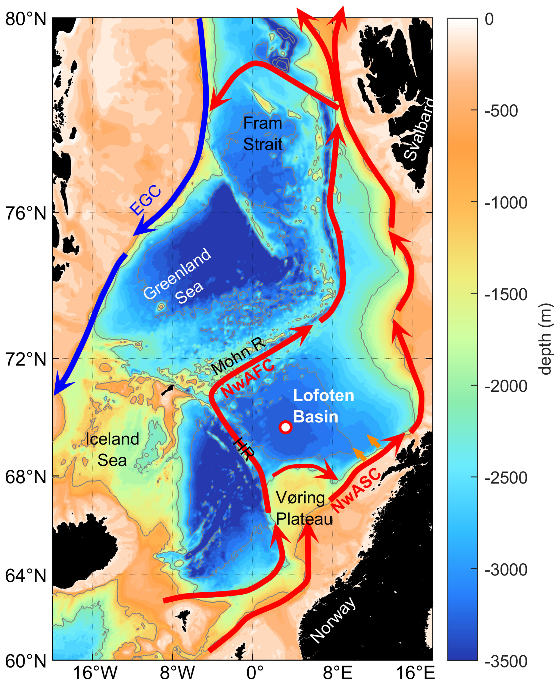
Figure 1 The Nordic Seas. Bathymetry is shown in colour, with grey contour lines every 1000 m. The coloured arrows represent the main circulation patterns, with the warm Norwegian Atlantic Current in red and the cold East Greenland Current (EGC) in blue. Small orange arrows indicate the region where warm anticyclonic eddies are shed from the NwASC. HR denotes the Helgeland Ridge, Mohn R denotes the Mohn Ridge, NwAFC denotes the Norwegian Atlantic Front Current, and NwASC denotes the Norwegian Atlantic Slope Current. The white circle with the red outline in the Lofoten Basin marks the mean position of the Lofoten Vortex.

Warm Atlantic Water enters the Lofoten Basin in two ways: from the south as the result of the separation of the two branches of the Norwegian Atlantic Current (Rossby et al., 2009b; Dugstad et al., 2019) and from the east via coherent anticyclonic mesoscale eddies shed from the NwASC near the Lofoten Escarpment (Köhl, 2007; Isachsen, 2015; Richards and Straneo, 2015; Volkov et al., 2015; Fer et al., 2020). After formation, these eddies propagate westward and transport heat towards the deeper part of the Lofoten Basin (e.g. Rossby et al., 2009b; Andersson et al., 2011). Raj et al. (2016) used satellite data from 1995 to 2013, together with data from surface drifters and Argo floats, to characterise the eddy field of the Lofoten Basin and inferred a generally cyclonic drift of eddies in the western Lofoten Basin with mean speeds of 5–6 km d⁻¹, consistent with previous analysis of the mid-depth circulation from Argo float trajectories by Voet et al. (2010). The eddy lifespan varied from days to months for both cyclonic and anticyclonic eddies, but a greater portion of the anticyclonic eddies were long-lived, and these long-lived anticyclonic eddies were found predominately in the western Lofoten Basin around the Lofoten Vortex (LV).

The LV, also known as the Lofoten Basin Vortex or the Lofoten Basin Eddy, is an apparently permanent oceanic anticyclonic eddy located in the deepest part of the Lofoten Basin (Søiland and Rossby, 2013; Yu et al., 2017). First observed in the 1970s (Ivanov and Korablev, 1995a), the LV consists of a core of warm, saline Atlantic Water which can reach as deep as 1200 m (Bosse et al., 2019). The deep mixing within the LV and the persistence of the LV influence water mass transformations regionally: within the LV, Atlantic Water has been found at depths several hundred metres deeper than in surrounding parts of the Lofoten Basin (Raj et al., 2015; Bosse et al., 2018).

The LV core is surrounded by a region of intense azimuthal velocities. These azimuthal velocities can reach 0.8 m s⁻¹ at 600–800 m depth, and relative vorticities are typically around −0.5f but sometimes reach as low as −0.9f, close to the theoretical limit for anticyclones (Bosse et al., 2019; Fer et al., 2018). The radius of the LV core is usually defined as the radius at the maximum azimuthal velocity R_v and has typically been found to be between 15–20 km based on acoustic Doppler current profiler (ADCP) measurements, glider cyclogeostrophic reconstruction, and Lagrangian RAFOS floats drifting at 500–800 m depth (Søiland and Rossby, 2013; Yu et al., 2017; Fer et al., 2018; Bosse et al., 2019). The LV also has a detectable signature in sea surface height. Raj et al. (2015) used a persistent sea level anomaly of at least 2 cm to detect the LV in 16 years of satellite altimetry data from 1995 to 2010. They found the radius of the LV to have a mean value of 37 km, but gridded satellite altimetry products are known to overestimate the LV radius as defined by the maximum azimuthal velocity (Yu et al., 2017). They also found the LV centre to be located between 69.5–70° N, 2.5–4.1° E (first and third quartiles). This is consistent with the LV locations found by Søiland and Rossby (2013), Yu et al. (2017), Fer et al. (2018), and Bosse et al. (2019).

Several authors have reported a multiple-core vertical structure in the LV, i.e. weakly stratified cores separated by layers of higher stratification, although single cores have occasionally been observed (e.g. Søiland and Rossby, 2013; Raj et al., 2015; Søiland et al., 2016; Yu et al., 2017; Fer et al., 2018; Bosse et al., 2019). Yu et al. (2017) and Bosse et al. (2019) discuss the varying vertical structure in terms of seasonal changes, using ocean glider observations of the LV taken between 2013–2015 and 2016–2017, respectively. During winter, strong cooling at the surface results in convective mixing reaching several hundred metres deep (though not as deep as 1000 m in the years they observed). Beginning in approximately April–May, surface warming creates a cap of restratified waters above the core which can extend down to approximately 200 m over the summer. When wintertime convection resumes, the upper water column is again homogenised as the mixed layer grows. As time progresses, the temperature and salinity properties of each wintertime core layer change gradually; the layers densify and are found deeper in the water column. The layer formed each winter is thus found above that of the previous winter, resembling vertical “stacking” (see, for example, Yu et al., 2017's Fig. 11). However, while the observations of Yu et al. (2017) and Bosse et al. (2019) suggest wintertime convection penetrating to a few hundred metres at most, Søiland and Rossby (2013) and Søiland et al. (2016) found highly homogenised water to ∼1000 m in July 2010 and September 2012, respectively, suggesting that convection penetrated to at least that depth during the preceding winter.

Based on ocean microstructure observations from a summer cruise, Fer et al. (2018) estimated the timescale to drain the volume-integrated total energy of the LV by the volume-integrated dissipation in the same radial and vertical (100–1400 m) extent of the eddy to be 𝒪(10) years. The turbulent dissipation rate was driven by strong shear below the swirl velocity maximum at the vortex rim and near-inertial waves trapped by the negative vorticity in the vortex core. Including additional processes of surface and bottom drag, Bosse et al. (2019) adjusted this timescale down to 3 years. Given that the LV has been observed for considerably longer periods than 3 years (especially the 16-year-long observation from the satellite data studied by Raj et al., 2015), it must therefore be maintained by processes which supply potential energy that overcomes the energy dissipation beyond a timescale of a few years.

Two mechanisms have been proposed to play a role in maintaining the structure and characteristics of the LV: wintertime deep convection (Ivanov and Korablev, 1995a, b) and the merging of mesoscale eddies into the LV (Köhl, 2007). Convection events are hypothesised to deepen the isopycnals below the vortex core, increase the radial density gradient, and intensify the azimuthal velocity, whereas eddy mergers are believed to increase vertical stratification and intensify the LV by compression and potential vorticity (PV) conservation (Trodahl et al., 2020). Various model studies have investigated these processes. In an idealised numerical case study, de Marez et al. (2021) concluded that the LV can survive thanks to a balance between mergers, convection, and bottom drag. Trodahl et al. (2020) studied the LV using the high-resolution, eddy-resolving Regional Ocean Modelling System (ROMS), a hydrostatic model with terrain-following coordinates with a horizontal resolution of 800 m and 60 vertical layers. They investigated the mesoscale eddy merging process and identified three to four merger events each year, with no clear seasonal bias. This is in contrast to two previous modelling studies, both using the Massachusetts Institute of Technology general circulation model with a horizontal resolution of 4 km: that of Köhl (2007), who also found three to four merging events per year but with slightly more mergers occurring during the period February–May and none in November–December, and the study of Belonenko et al. (2017), who identified one to two mergers per year, with a distribution skewed towards wintertime. Detailed merger observations in the water column have not been reported to date; however, Bosse et al. (2019) indirectly deduced a merger in winter when the LV core's heat content increased by the amount contained in a typical mesoscale anticyclonic eddy contemporaneously with the restratification of the upper core.

While the supporting role of convection cannot be ruled out, Trodahl et al. (2020) concluded that the LV is mainly maintained through repeated merging events. Incoming eddies approach the LV, begin to co-rotate with it, become elongated and wrap around the LV, and are eventually absorbed by it. The LV is typically denser at its core than incoming eddies because the LV is subject to prolonged cooling periods, whereas the incoming eddies are shorter-lived and have not had time to lose as much heat since they were spun out from the NwASC. Thus, the merging process modelled by Trodahl et al. (2020) frequently results in a double-core vertical structure at the end of the merging process, which can persist for weeks to months, because the lighter incoming eddy is stacked above the original LV core (see Trodahl et al., 2020's Fig. 14). This accords well with the eddy merging processes observed by Garreau et al. (2018) in the Mediterranean Sea, Belkin et al. (2020) in the Gulf Stream, and Rykova and Oke (2022) in the Tasman Sea; the latter authors also found that the merging of two eddies of different densities led to vertical stacking. In the LV, the cores of the vertically aligned denser vortex and the lighter merging eddy are subsequently fused through vertical convection (Trodahl et al., 2020). However, when the incoming eddy is of a similar density to the LV, the result is a single LV core. During the merging process (irrespective of whether it results in a single or double core), the combined vortex becomes more vertically stratified, is intensified by compression and PV conservation, and expels some low-PV fluid. Wintertime convection serves mainly to vertically homogenise and densify the LV impacting its potential energy, whereas merging events have the strongest impact on intensifying it by means of the transfer of kinetic energy.

Vortex merging is an active field of research, though mostly through numerical simulation given the difficulty of in situ observations of such transient processes. During merging, two like-signed eddies (i.e. both anticyclonic or both cyclonic) come into close contact with each other and then form either one larger eddy or two asymmetrical eddies, depending on initial conditions (see, for example, Dritschel, 2002; Meunier et al., 2002; Reinaud and Dritschel, 2002; Bambrey et al., 2007; Özugurlu et al., 2008). While most studies of this process consider isolated vortex mergers, i.e. omitting the influence of environmental factors such as neighbouring eddies or large-scale currents, de Marez et al. (2020) deduced that merging is influenced by the β effect and surrounding eddies. Efforts to include more physical effects in studies of vortex mergers are often impaired by the lack of observations of these processes. The LV offers an ideal location to capture in situ observations of merger events. However, apart from the current study, we are not aware of any direct in situ observations of a merger event.

In December 2022, the Surface Water and Ocean Topography (SWOT) satellite was launched. It employs a Ka-band radar interferometer (KaRIn) providing maps of sea surface height (SSH) at a native horizontal resolution of 250 m and noiseless products at 2 km within two swathes, each 60 km wide, separated by a 20 km gap; in the middle of the gap, sea level is measured by a conventional nadir altimeter (Fu et al., 2024). The SWOT satellite's fast sampling calibration and validation phase (henceforth the Cal/Val phase) lasted from 29 March to 10 July 2023: during this time, the satellite passed over the same locations on the planet each day. One of the crossover points was located above the mean position of the LV (Fig. 2); thus, this area was observed twice per day, once on the ascending track and once on the descending track. SWOT offers a significant increase in resolution over nadir altimeters such as Jason, Sentinel and TOPEX/Poseidon. While such satellites have improved our knowledge of mesoscale eddies on horizontal scales O(50–500) km, they can miss smaller mesoscale eddies and nearly all submesoscales (Klein et al., 2019). Zhang et al. (2024) have demonstrated that SWOT is easily able to resolve submesoscale eddies with radii as small as 16 km and sea level anomaly amplitudes as small as 2 cm; thus, it should have no difficulty in resolving the LV. This unprecedented resolution offered the opportunity to observe the LV, and nearby eddies, as never before, and thus coincident glider missions were planned to collect observations from the LV during the SWOT Cal/Val phase, participating in the global effort of in situ data collection during this crucial phase (d'Ovidio et al., 2019).

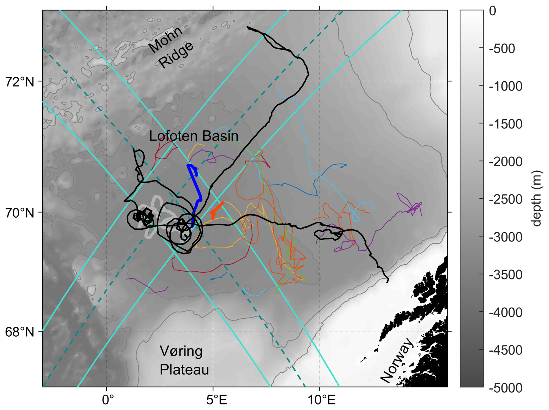
Figure 2 The Lofoten Basin, showing the path of SG563 (black); the position of the LV for the time period 1 January–31 June 2023 (grey), taken from the altimetric Mesoscale Eddy Trajectories Atlas (META3.2exp NRT); and the outer edges of the Surface Water and Ocean Topography (SWOT) swathes (turquoise) and the SWOT nadirs (dark cyan). Bathymetry contours are every 1000 m. Coloured lines are the tracks of mesoscale eddies, also from META3.2exp NRT. We include all tracks where at least part of the track lies within the region 68.5–71.5° N, 0–10° E in the time period 1 January–30 June 2023. Two eddy tracks are highlighted, which will be discussed further in the text: the thick blue line is eddy A, and the thick orange-red line is eddy B.

In this paper, we present in situ observations of a mesoscale eddy merging into the Lofoten Vortex, which took place between 5–16 April 2023. Subsurface observations are supplemented by the measurements from SWOT. Section 2 presents the in situ and satellite data and details the methods used to characterise the LV. Section 3 presents the results, focusing on the merger of a mesoscale eddy into the LV in April 2023, though we also infer a previous merger in March 2023. Section 4 contains the discussion and conclusions.

2 Data and methods

2.1 In situ data

Hydrographic data were acquired using the Seaglider SG563, which was deployed from RV Johan Hjort on 19 January 2023 and recovered on 8 June 2023 by RV G.O. Sars, completing 620 dives in total. Seagliders are small, autonomous, remotely piloted, buoyancy-driven vehicles which profile to a maximum depth of 1000 m in a sawtooth pattern (Eriksen et al., 2001; Testor et al., 2019). SG563 carried a CT sail measuring conductivity and temperature. Sampling occurred every 10 s (∼1 m vertical resolution at typical vertical speeds of ∼0.1 m s⁻¹) in the upper part of the water column to 300 m and every 15 s (∼1.5 m vertical resolution) below that. SG563 was deployed on the eastern side of the Lofoten Basin and proceeded west, arriving in the vicinity of the LV on 3 March. It completed approximately 200 dives in the vicinity of the LV in the period between 3 March–7 May and then proceeded northeast before being recovered (Fig. 2).

The raw data were processed using the University of East Anglia Seaglider toolbox (https://bitbucket.org/bastienqueste/uea-seaglider-toolbox/ commit 025191f, last access 11 January 2023). The Seaglider hydrodynamic flight model was tuned following Frajka-Williams et al. (2011). Depth-averaged currents (DACs) were calculated from the difference between the glider's flight path found from GPS positions at the beginning and end of each dive and the glider's flight path relative to the water as calculated using dead reckoning and the Seaglider hydrodynamic flight model. The thermal lag of the CT sail was corrected following the methods of Garau et al. (2011). Occasional poor-quality data (e.g. from poor flushing of the conductivity cell when the glider is moving slowly) were flagged and discarded, and outliers in the salinity profiles were removed using a three-run Hampel filter (Liu et al., 2004); together, these account for 3 % of the total data collected. Conservative Temperature and Absolute Salinity were calculated using the thermodynamic equation of sea water (IOC et al., 2010), and all references to temperature and salinity from this point onward should be taken to mean Conservative Temperature and Absolute Salinity. The potential density anomaly (σ₀) was calculated relative to the surface pressure.

Temperature and salinity were calibrated against available ship conductivity, temperature, and depth (CTD) data managed by the Institute of Marine Research in Bergen, Norway. CTD casts were chosen which were collected within 5 km and 3 d of a glider profile; the top 300 m was excluded to avoid the rapidly changing effects of surface forcing, and data within any pycnoclines were also excluded. These selection criteria were chosen to maximise the number of profiles used for calibration while still ensuring that the matching profiles were sampling the same water masses. In particular, the selection criteria ensured that glider profiles within the LV were matched to CTD profiles within the LV, whereas glider profiles outside the LV were matched to CTD profiles outside the LV since the water column properties inside and outside the LV are significantly different. This led to a total of 13 glider–CTD profile pairs being used for calibration. Salinity was corrected by an offset of 0.021 g kg⁻¹, and temperature was corrected by an offset of 0.061 °C. The glider data are available from the Norwegian Marine Data Centre, including the final, quality-controlled data and the associated raw data files (Damerell et al., 2024).

2.2 Characterisation of the LV

Seagliders have a navigation mode which is well suited for piloting inside eddies: steering relative to the DAC of the previous dive. By steering at 90° to the previous dive's DAC, the glider will spiral into the core of the LV, which can be easily identified by pilots based on the deep core of warm Atlantic Water. Once the core is reached, the glider can be commanded to steer at 270° to the previous dive's DAC and will spiral out of the LV. These spiralling tracks, henceforth referred to as vortex realisations, take approximately 4–6 d to complete. This method has been used to study the LV previously (Yu et al., 2017; Bosse et al., 2019).

Each LV realisation aims to characterise the LV's hydrography and dynamics in radial section. First the glider's DACs are used to detect the LV centre by minimising a cost function applied to a rolling window of four consecutive DACs to find the position where DACs are most perpendicular to the vectors joining their positions to the eddy centre (Bosse et al., 2015). Detected centres are only kept when the glider is reasonably close to the LV's core, where the cost function minimum is properly defined by closed contours. Geographical coordinates of glider sampling points are then transformed into cylindrical coordinates $(r,\mathit{\theta },z)$, neglecting the eddy's ellipticity, with r the radial distance from the LV centre, θ the azimuthal angle, and z the depth. As in Bosse et al. (2019), temperature, salinity and DAC data are bin-averaged on a regular grid (3 km in radial distance, 5 m in vertical) and optimally interpolated using correlation scales typical of the LV's radius (L_r=15 km) and of the seasonal thermocline thickness (L_z=15 m). In our analysis, we used the optimally interpolated radial sections. Measurements along the dives of the glider, before this bin-averaging and optimal interpolation, are shown in Fig. B1 to highlight the lateral resolution of the profiles. The cyclogeostrophic balance is finally solved for azimuthal velocities (see Appendix A in Bosse et al., 2016), as the strong vorticity of the LV implies important effects of the non-linear centrifugal force.

The following LV characteristics are described for each realisation. The radius R_v is defined as the radial distance of the velocity maximum v_m. Water properties of the inner core and outside the LV are defined as the mean profiles located at a distance inferior to $\mathrm{2}/\mathrm{3}{R}_v$ and between 3R_v and 5R_v, respectively. LV vorticity is obtained in cylindrical coordinates, as in Bosse et al. (2019), using

$$\begin{array}{}\text{(1)}& {\displaystyle }{\displaystyle }\mathit{\zeta }(r,z)={\displaystyle \frac{\mathrm{1}}{r}}\left({\displaystyle \frac{\partial \left(r{v}_{\mathit{\theta }}\right)}{\partial r}}\right),\end{array}$$

where v_θ(r,z) is the azimuthal velocity, and the Rossby number $\mathit{\text{Ro}}=\mathit{\zeta }/f$ is the vorticity normalised by f, the Coriolis parameter. PV (${\mathrm{m}}^{-\mathrm{1}}{\mathrm{s}}^{-\mathrm{1}}$) is finally calculated as

$$\begin{array}{}\text{(2)}& {\displaystyle }{\displaystyle }\text{PV}(r,z)={\displaystyle \frac{\mathrm{1}}{g}}\left[N^{\mathrm{2}}(f+\mathit{\zeta })-\left({\displaystyle \frac{\partial v_{\mathit{\theta }}}{\partial z}}\right)\left({\displaystyle \frac{\partial b}{\partial r}}\right)\right],\end{array}$$

with $b=-{\mathit{\sigma }}_{\mathrm{0}}/\left({\mathit{\rho }}_{\mathrm{0}}g\right)$ the buoyancy, σ₀ the potential density anomaly, g=9.81 m s⁻² the gravitational acceleration, ρ₀=1028 kg m⁻³ a reference seawater density, and $N^{\mathrm{2}}=\partial b/\partial z$ the buoyancy frequency.

2.3 Altimetry

Level-3 SWOT satellite altimetry data were retrieved in their last validated version (v2.0.1, CNES, 2024) during the Cal/Val phase from 29 March 2023 to 10 July 2023 for tracks 5 (descending pass) and 14 (ascending pass) from the AVISO ftp server (Dibarboure et al., 2025) as these two tracks have a cross-over in the LV region. Fields of noiseless Sea Surface Height Anomaly (SSHA) and Mean Dynamic Topography (MDT) at 2 km resolution were used to infer Absolute Dynamic Topography (ADT) as follows: $\text{ADT}=\text{SSHA}+\text{MDT}$. Here, we remove the monthly average of the ADT over the study area of 68.5–71.5° N, 0–6° E and refer to what remains as the local ADT anomaly (ADTa). Horizontal velocities (u,v) satisfying the cyclogeostrophic balance were computed using Jaxparrow open-source software (Bertrand et al., 2024). The variational approach of this new method allows one to solve the gradient wind balance, whereas the iterative method previously developed by Penven et al. (2014) for larger-scale gridded altimetry does not consistently converge when applied to high-resolution SWOT data. Relative vorticity maps were finally obtained from cyclogeostrophic velocities by calculating

$$\begin{array}{}\text{(3)}& {\displaystyle }{\displaystyle }\mathit{\zeta }={\displaystyle \frac{\partial v}{\partial x}}-{\displaystyle \frac{\partial u}{\partial y}}.\end{array}$$

In order to refine the characteristics of the LV and the merging eddy during this critical period, we applied an eddy detection method to the SWOT-based high-resolution ADT in April 2023. For each individual SWOT swath sampled during the Cal/Val phase, the maximum of ADT in the study area was considered to be the LV centre position, (x_LV,y_LV). The parameters $(A_{\text{LV}}^{\mathrm{0}},A_{\text{LV}},R_{\text{LV}})$ of an idealised Gaussian eddy,

$$\begin{array}{ll}{\displaystyle }{\text{ADT}}_{\text{LV}}(x,y)=& {\displaystyle }{A}_{\text{LV}}^{\mathrm{0}}\\ \text{(4)}& {\displaystyle }& {\displaystyle }+A_{\text{LV}}{\exp }^{-\left[(x-x_{\text{LV}}{)}^{\mathrm{2}}+(y-y_{\text{LV}}{)}^{\mathrm{2}}\right]/\mathrm{2}{R}_{\text{LV}}^{\mathrm{2}}},\end{array}$$

were then derived from SWOT ADT. $A_{\text{LV}}^{\mathrm{0}}$ was set as the median of ADT in the far-field, considered to be the region between 100–150 km away from the LV centre. A_LV was set as the maximum of ADT (i.e. at the centre of the LV). Finally, R_LV was inferred from a least-square regression between the observed ADT and the Gaussian model in a region less than 45 km from the LV centre. Note that this definition is consistent with a radius of maximum azimuthal velocity. This procedure was repeated on ADT−ADT_LV in order to characterise the approaching eddy $\left[\right(x_{\mathrm{B}},y_{\mathrm{B}}),A_{\mathrm{B}}^{\mathrm{0}},A_{\mathrm{B}},R_{\mathrm{B}}]$. As will be discussed below, the approaching eddy is eddy B, whose track is shown in Fig. 2. To avoid outliers and detection at the swaths' edges, these estimates were not considered in the analysis when less than 75 % of a disc of radius R_LV or R_B was covered by SWOT data and when the root mean square error between the Gaussian model and the measured ADT was larger than 5 cm in a disc of 100 km radius. The eddies' dynamical intensity was then characterised in terms of maximum Rossby number at the eddy centre by resolving the cyclogeostrophic balance for the Gaussian model:

$$\begin{array}{}\text{(5)}& \begin{array}{rl}R{o}^{max}& =-\mathrm{1}+\sqrt{\mathrm{1}-\mathrm{4}g{A}_i/f^{\mathrm{2}}{R}_i^{\mathrm{2}}}\\ \text{for}R{o}_{\mathrm{geo}}^{max}& =-\mathrm{2}g{A}_i/f^{\mathrm{2}}{R}_i^{\mathrm{2}}>-\mathrm{0.5}\\ \text{and}R{o}^{max}& =-\mathrm{1}\text{otherwise};\end{array}\end{array}$$

with $i=(\text{LV},\mathrm{B})$ and with $R{o}_{\text{geo}}^{max}$ the maximum Rossby number in geostrophic balance. It is worth noticing that the R_LV found with this method is about 30–35 km, which is larger than the glider-inferred R_v but is coherent with previously reported LV radii inferred from satellite data. This larger radius from the satellite data than from the in situ glider observations is most likely due to the Gaussian fit smoothing the finer-scale velocity signal of the core.

A typical error for the amplitude estimate (A_i) was estimated by examining the distribution of the background ADT signal ($A_i^{\mathrm{0}}$) over the merging period, leading to an error of 2 cm. Error in the radius estimate could be related to SWOT gridded product resolution; hence, we chose an error of 2 km for R_i. These error estimates were then propagated to Ro^max using its mathematical definition.

Eddy tracks were taken from the altimetric Mesoscale Eddy Trajectories Atlas (META3.2exp NRT, henceforth META3.2), which is produced by SSALTO/DUACS and distributed by AVISO+ (https://www.aviso.altimetry.fr/, last access: 14 August 2024) with support from CNES (France), in collaboration with IMEDEA (Spain) (Mason et al., 2014; Pegliasco et al., 2022). This dataset uses data from previous-generation altimetric satellites such as Jason, Sentinel, and TOPEX/Poseidon and does not incorporate SWOT data. We show only those tracks where at least part of the track lies within the region 68.5–71.5° N, 0–10° E in the time period of 1 January–30 June 2023 (Fig. 2). Two of these eddy tracks will be discussed in this paper: eddy A, which was tracked from 17 February to 12 March and is shown as a thick blue line in Fig. 2, and eddy B, which was tracked from 21 March to 4 April and is shown as a thick orange-red line in Fig. 2. Using these data allows us to extend the period in which we have data on eddy movements before the start of the SWOT Cal/Val phase.

2.4 Surface forcing data

Surface forcing data were taken from the ECMWF ERA5 reanalysis (Hersbach et al., 2023) and are shown in Fig. 3. ERA5 has a temporal resolution of 1 h and a horizontal resolution of 31 km. Each of the surface forcing variables was averaged over the area 69.5–70° N, 2.5–4.1° E (i.e. over 21 grid points), covering the typical variability in the location of the LV. This also agrees well with the vortex centre locations found in our data (see below). Mean net surface heat flux (Q_net, in W m⁻²) was then calculated as the sum of the short-wave, long-wave, sensible and latent heat fluxes. The mean net surface freshwater flux (FW_net, in kg m⁻²) was calculated as the mean total precipitation rate minus the mean evaporation rate.

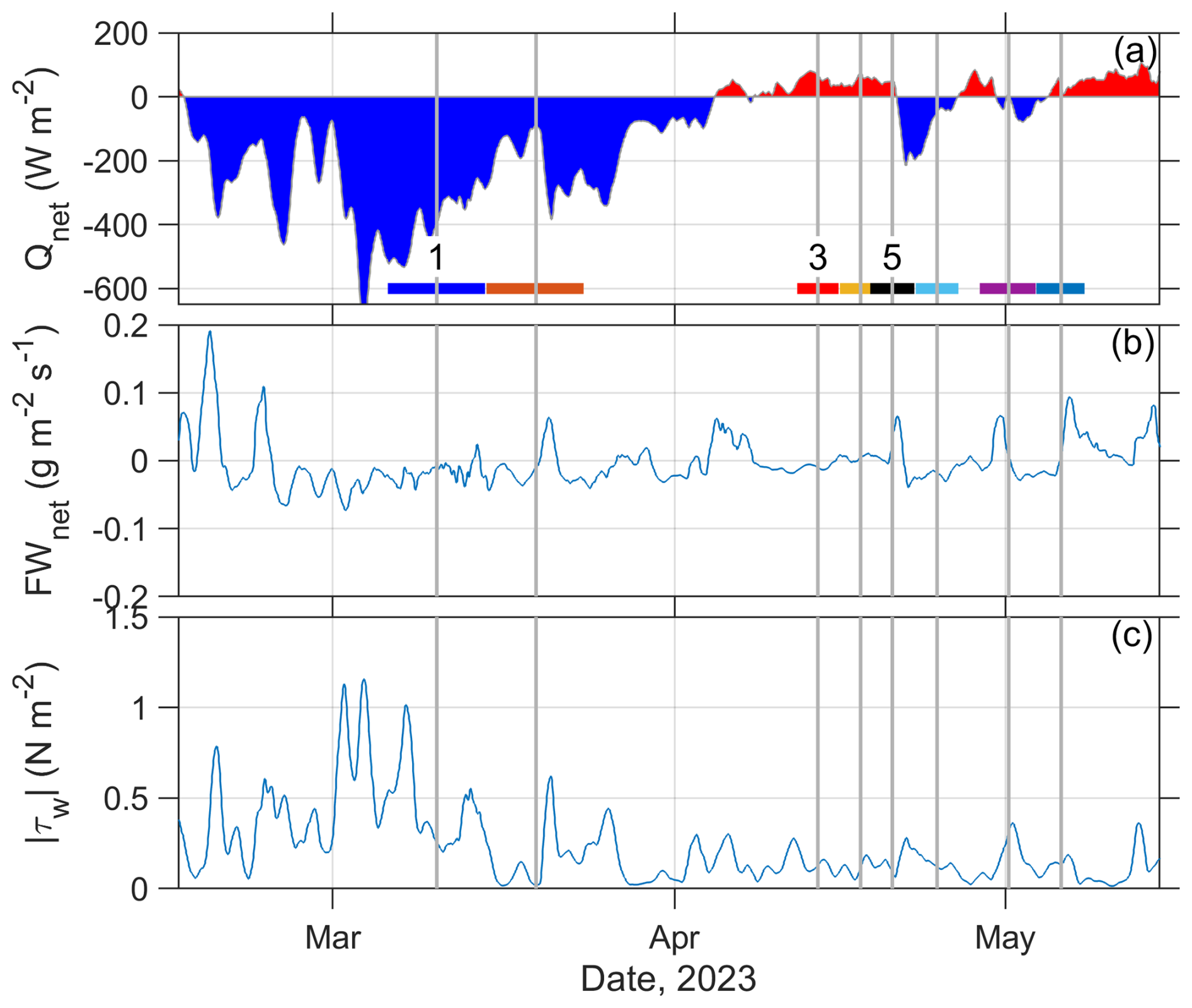
Figure 3 Surface forcing from ERA5, as described in Sect. 2.4. Daily averaged (a) net surface heat flux, (b) net surface freshwater flux, and (c) wind stress. Vortex realisations are marked by the coloured bars along the bottom of (a), and realisations 1, 3, and 5 are labelled. In all panels, vertical grey lines mark the mean date of each vortex realisation.

2.5 Error analysis of in situ glider data

To assess the sensitivity of the derived variables (e.g. azimuthal velocity maximum, relative vorticity, Rossby number) to various sources of uncertainty, we conducted a series of Monte Carlo simulations (Mooney, 1997), each isolating a specific source of error. For the measurement uncertainties of temperature and salinity, we generated 1000 sets (i.e. temperature and salinity) of perturbed data fields by adding normally distributed errors, with a prescribed standard deviation, to each measurement point. Each set of perturbed fields is then analysed by applying transformation into cylindrical coordinates, binning, optimal interpolation, and calculations as required to obtain the derived variables, exactly as in Sect. 2.2, giving 1000 estimates of each derived variable. The measurement uncertainty of the DACs is treated in the same way. Assessing the errors introduced by the assumption of axial symmetry involved applying scaling factors to the radial distances from the centre of the LV to profiles and DAC measurements and again generating 1000 realisations. These scaling factors were inferred from the vortex ellipticity seen in the SWOT data. Further details can be found in Appendix A. We report the mean, standard deviation and 95 % confidence intervals of the resulting distributions obtained from the 1000 estimates for each source of uncertainty.

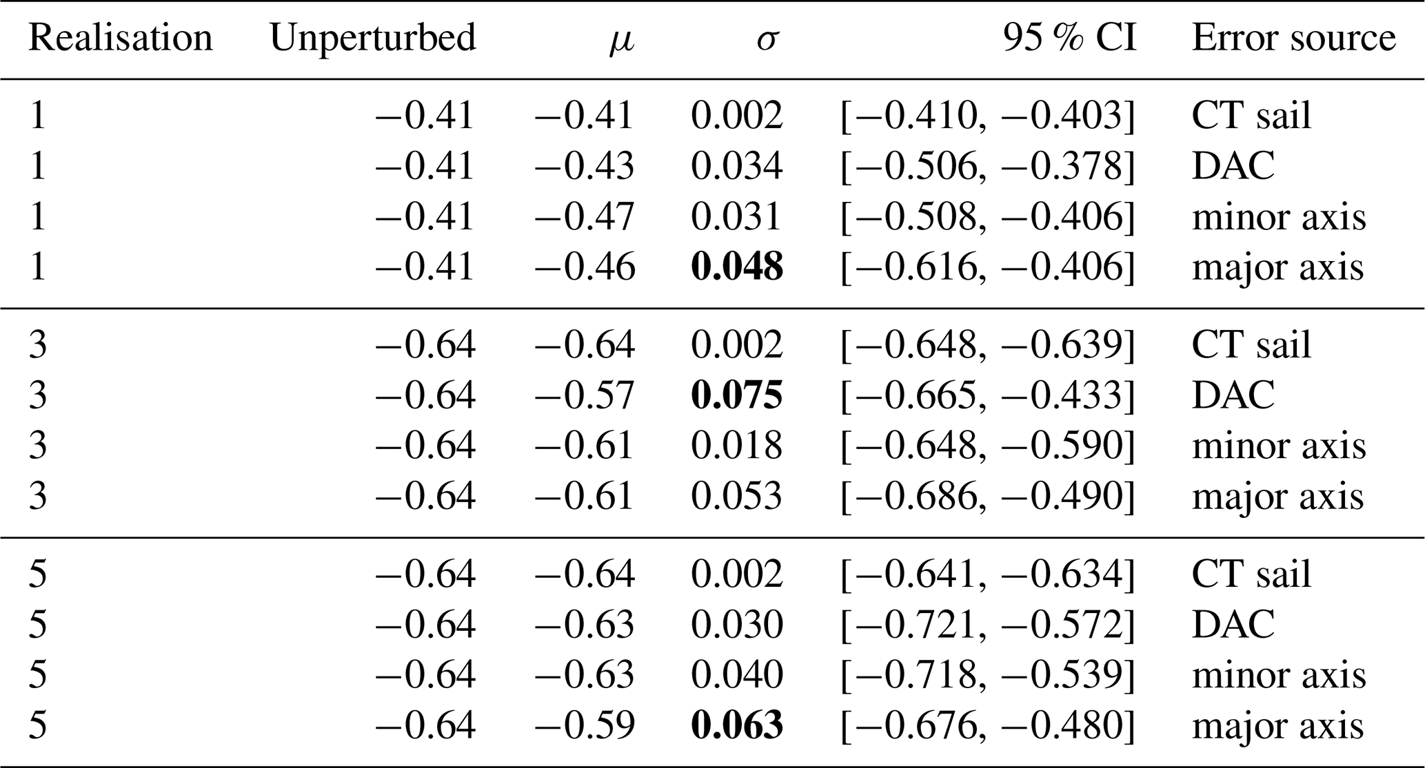
The results from this error analysis are detailed in Tables A1 and A2 in Appendix A. The errors from the CT sail measurement uncertainty are trivially small, but those from the DAC measurement uncertainty and from the assumption of axial symmetry are significant. When stating errors within the body of this paper, we give a conservative error estimate using the largest standard deviation in each case. For vortex realisation 3, the largest standard deviation for the maximum azimuthal velocity is derived from the DAC measurement uncertainty. In all other cases, the largest standard deviation is found from the assumption of axial symmetry, specifically from assuming that the glider's transect was aligned with the major axis of the LV ellipse. Thus the errors stated below may be considered to be the “worst case” and are likely to be an overestimate of the true uncertainty.

3 Results

SG563 visited the LV four times in the period March–May 2023 for a total of eight vortex realisations. Three of these realisations will be the focus of this paper: realisation 1, sampled between 5–14 March, which shows the late-winter properties of the LV; realisation 3, sampled between 12–15 April, which is the period when an eddy merged into the LV; and realisation 5, sampled between 18–22 April, which shows the effect of the merging. Radial sections of selected variables for these vortex realisations are shown in Fig. 4, followed by average profiles in the core and outside the LV in Fig. 5, together with their Θ–S_A diagrams. Radial sections of Θ and S_A along the dives before optimal interpolation (Fig. B1), Θ–S_A diagrams of individual profiles (Fig. B2), and the radial sections using density as a vertical coordinate (Fig. B3) are shown in Appendix B for reference. We do not show the other realisations because they do not add to the results presented here. In particular, because the glider spirals into the LV in each odd-numbered realisation and then out of the LV in the following even-numbered realisation, the glider dives in the centre of the LV at the start of each even-numbered realisation follow immediately after those at the end of the preceding odd-numbered realisation, and the properties of the LV core do not change significantly in such a short space of time. Core profiles from each even-numbered realisation are thus extremely similar to the core profiles from the preceding odd-numbered realisation and are not shown.

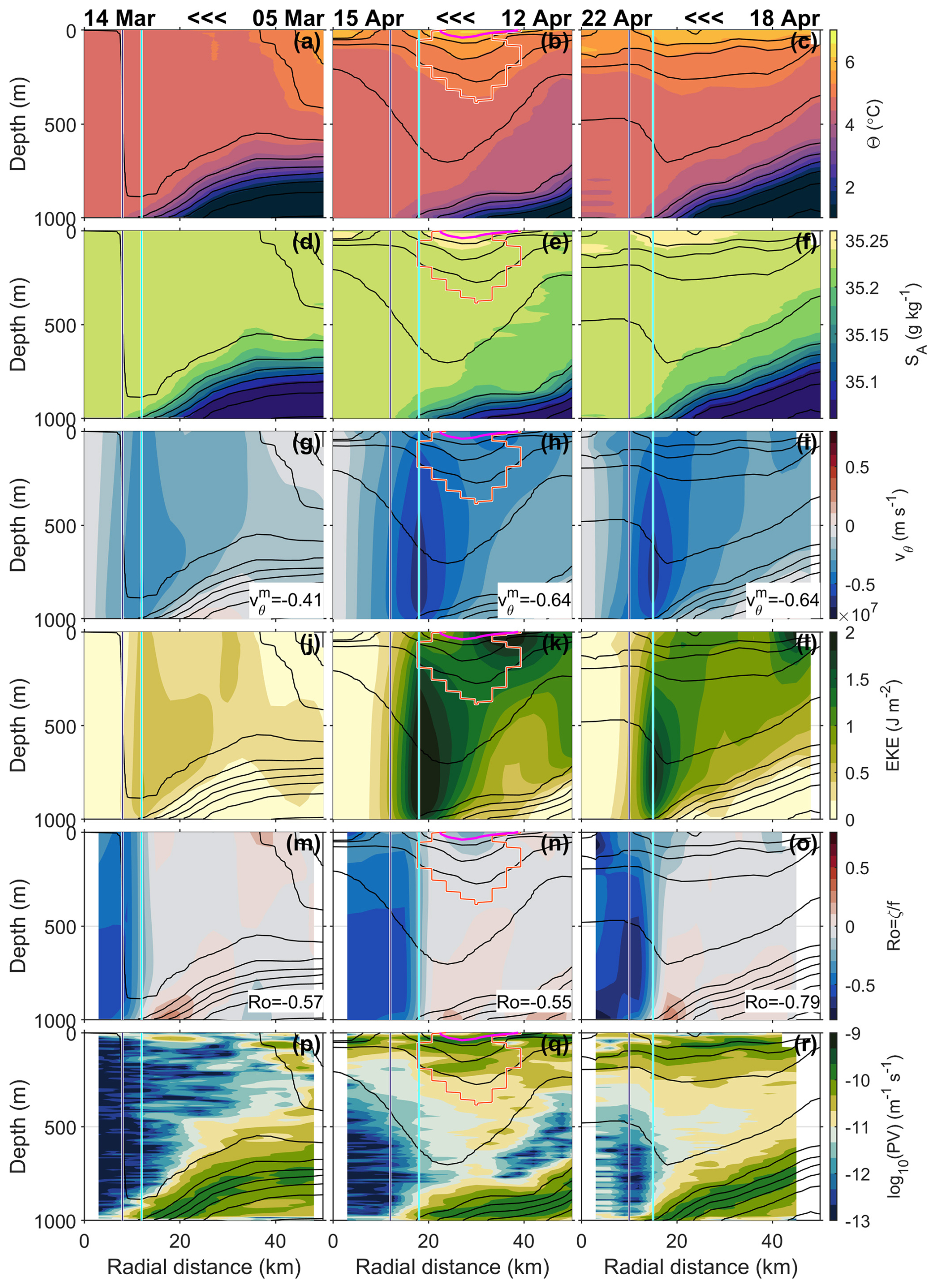
Figure 4 Sections through the LV: the first column shows realisation 1 between 5–14 March, the second column shows realisation 3 between 12–15 April, and the third column shows realisation 5 between 18–22 April. Note that, because the glider is travelling from outside the LV towards the centre of the LV in each of these realisations, the left-hand side of each panel is later in terms of date than the right-hand side, as indicated by the labels at the top of each column. (a–c) Temperature; (d–f) salinity; (g–h) azimuthal velocity, with the maximum ${\mathrm{v}}_{\mathit{\theta }}^{\mathrm{m}}$ value indicated in the bottom right; (j–l) eddy kinetic energy; (m–o) Rossby number $\mathit{\text{Ro}}=\mathit{\zeta }/f$, with the minimum Ro value indicated in the bottom right; (p–r) potential vorticity (PV). Θ–S_A diagrams for these realisations can been seen in Fig. B2. Black contours in all panels show the potential density anomaly (σ₀) every 0.04 from 27.6 to 28.0 kg m⁻³. Vertical cyan lines on all panels show the radius of the core R_v. Vertical blue lines show $\mathrm{2}/\mathrm{3}{R}_v$. In the second column, the orange-red contour outlines eddy B, which is merging into the LV, and the magenta contour marks the σ₀=27.6 kg m⁻³ isopycnal.

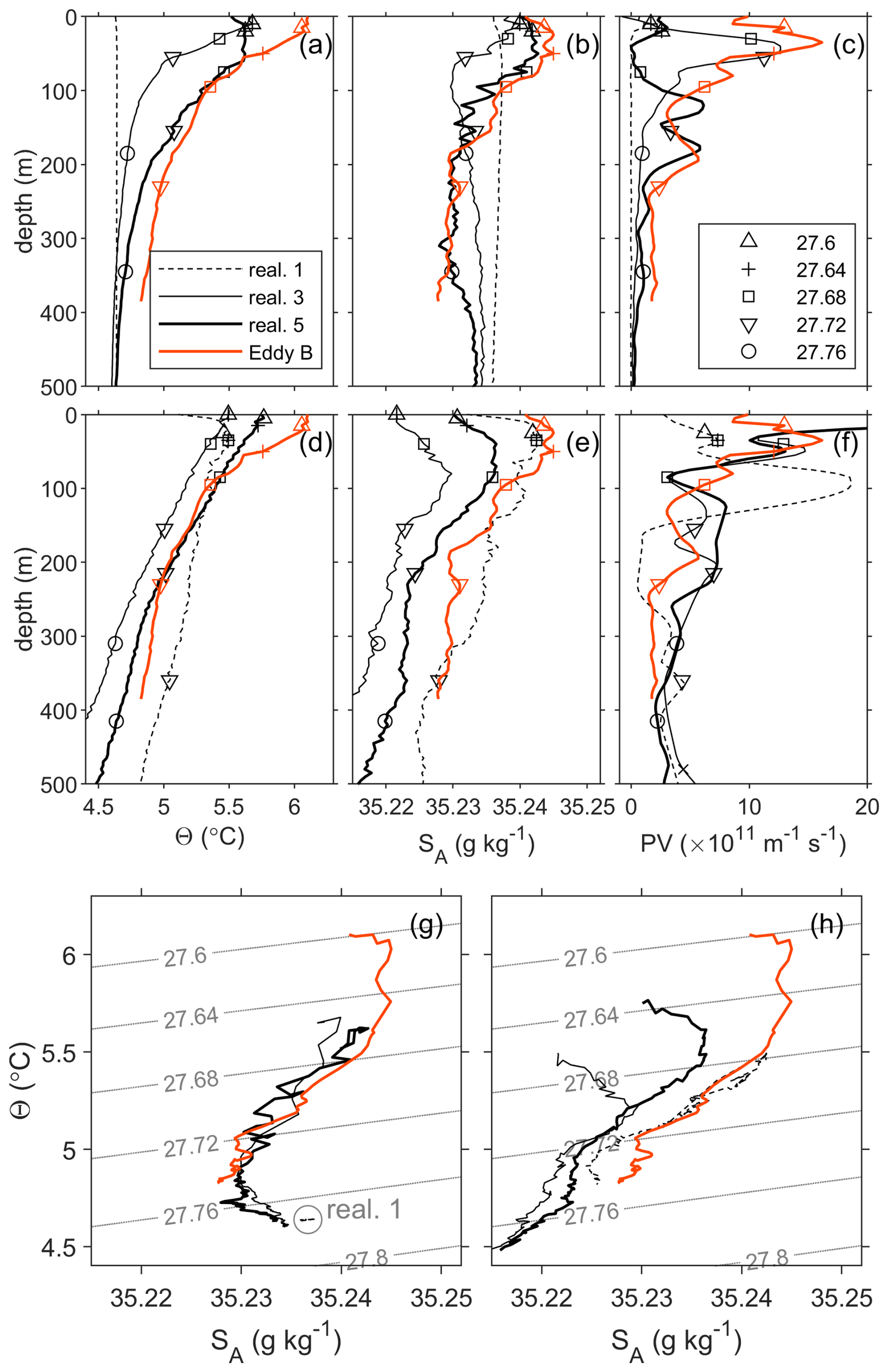
Figure 5 Average water profiles in the top 500 m in the core of the LV (a–c) and outside the LV (d–f) for (a, d) temperature, (b, e) salinity, and (c, f) PV (multiplied by 10¹¹ for display purposes) and Θ–S_A diagrams of the top 500 m (g) in the LV core and (h) outside the LV. In each panel, dashed black lines show properties during realisation 1, 5–14 March; thin solid black lines show properties during realisation 3, 11–15 April; and thick black lines show properties during realisation 5, 18–22 April. Orange-red lines show the properties of eddy B, as defined in the main text. Markers in (a–f) depict different potential density anomalies on each profile, as given by the legend in (c). There are no markers on the core profile for realisation 1 because the entire profile lies between σ₀=27.772 and σ₀=27.773 kg m⁻³.

3.1 Late-winter conditions in the LV

In realisation 1, (Fig. 4, first column) the LV displays a well-mixed winter core with weakly stratified waters extending to 1000 m. Core profiles of temperature, salinity and PV are vertically uniform, and the density is well-mixed throughout the water column to 1000 m (Fig. 5). The core of the LV (radial distance of about 10–15 km in Fig. 4) is surrounded by a rim of increased azimuthal velocity, reaching a maximum of 0.4(±0.05) m s⁻¹ (Fig. 4g). Low PV is seen throughout the core from the surface to 1000 m (Fig. 4p). The shape of the low-PV area is lens-like but extends further out of the core between depths of approximately 50–500 m. The relative vorticity of the core is strongly anticyclonic, reaching $-\mathrm{0.57}(\pm \mathrm{0.12})f$ (Fig. 4). Note this is not a double-core vertical structure, such as many previous observations have seen (e.g. Yu et al., 2017; Fer et al., 2018; Bosse et al., 2019), but instead shows the result of winter mixing to at least 1000 m, similar to the earlier observations of Søiland and Rossby (2013) and Søiland et al. (2016). In March, prior to realisation 1, net surface heat losses were large (−400 to −650 W m⁻²), and wind stress exceeded 1 N m⁻² in several episodes, suggesting strong convection and atmospheric forcing (Fig. 3).

Outside the LV, profiles are typical of the Lofoten Basin, with a thin (approximately 20 m), fresh and cold surface layer and somewhat warmer and saltier waters beneath, which then gradually cool and freshen towards 1000 m (Fig. 4). The change in properties is almost density-compensating from the surface to 100 m (Figs. 4 and B3), and even to 400 m the density changes are small.

3.2 Comparing centre positions

The LV is clearly visible as a persistent, approximately circular area of elevated ADTa (Fig. 6) and strongly anticyclonic vorticity (Fig. 7), centred between 69.75–70° N, 2.5–4° E (consistent with the LV positions in the literature), throughout the SWOT Cal/Val phase. The positions of the LV from META3.2 (grey triangles with black outlines in Fig. 6) are close to the positions of maximum ADT in the SWOT data (grey dots with black outlines in Fig. 6, henceforth SWOT-derived centre positions), with an average separation of 6.0 km in April 2023. On seven days (14–17 and 21–23 April 2023), positions for the centre of the LV were also found from the glider data, as described in Sect. 2.2. On these days, the average distance between the LV centre positions from META3.2 and the glider-derived LV centre positions was 4.8 km, and the average distance between the SWOT-derived and glider-derived LV centre positions was 4.9 km. At first glance, this might suggest that META3.2 gives comparable estimates of the centre position of the LV to the SWOT-derived centre positions. However, it is worth noting that, firstly, the sample size is small; secondly, the META3.2 positions are daily estimates, the SWOT-derived positions come from the time of a particular pass of the SWOT altimeter, and the glider-derived positions are based on data from four dives covering a period of approximately 20 h, and thus they do not all represent equivalent time periods; thirdly, the glider-estimated centre positions rely on an assumption of axial symmetry, but there are some slight distortions from circular in the ADTa contours (Fig. 6) which will cause some slight alterations in the glider-estimated centre positions. Given these provisos, it seems reasonable to conclude that the META3.2, SWOT-derived, and glider-estimated centre positions are all within a few kilometres of each other, but we cannot say that one position estimate is better than the others during the limited period considered.

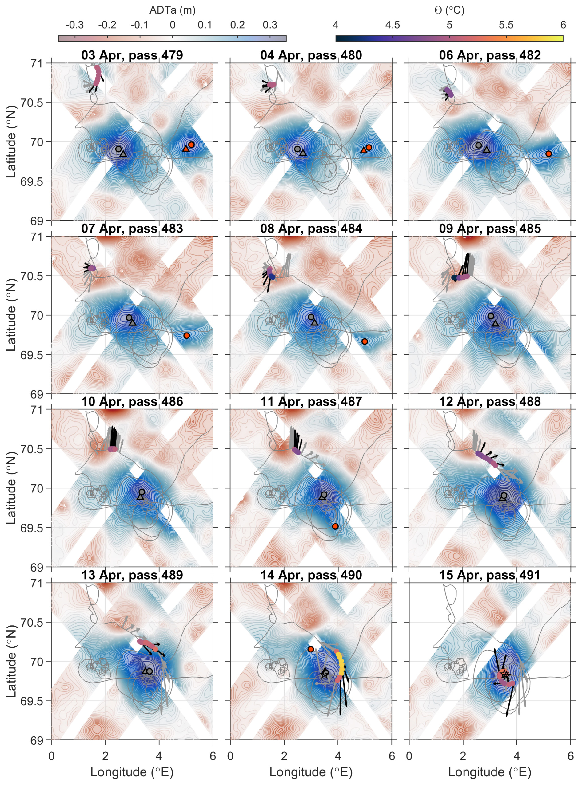
Figure 6 ADTa from the SWOT altimetry (coloured contours and shading) from 3 to 15 April 2023. Note that 5 April is not shown but was extremely similar to 4 April. Dates and SWOT pass numbers are given above each panel. The grey line shows the whole-mission path of SG563, and coloured dots along this path show the average temperature of the top 100 m for profiles taken on the date given above each panel. Black arrows show the DACs measured that day, and grey arrows show the DACs for the day before and after. The black stars on 14–15 April show the LV position detected by the glider (Sect. 2.2). Grey triangles with a black outline mark the daily position of the LV from META3.2, and orange-red triangles with a black outline mark the daily position of eddy B from META3.2, which is also shown as an orange-red track in Fig. 2. The last date given for this track was 4 April 2023; thus, its position is not shown for later dates. Grey dots with a black outline mark the position of the LV from the maximum ADT in the SWOT swath data, and orange-red dots with a black outline mark the position of eddy B from the SWOT swath data on days when the position met the eligibility criteria described in Sect. 2.3.

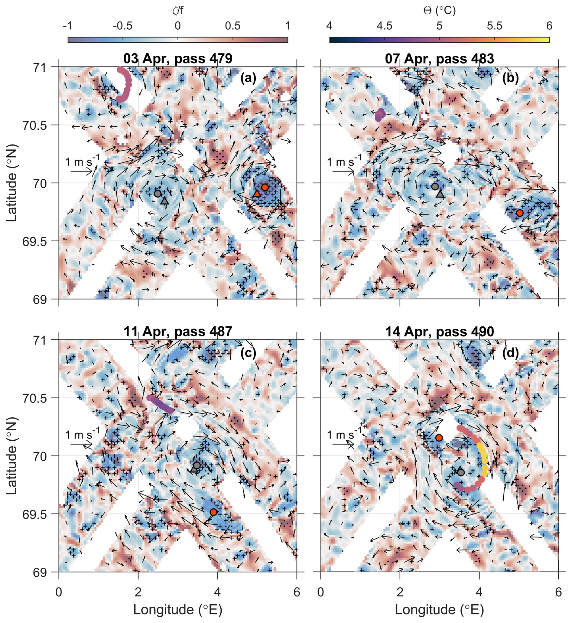
Figure 7 Relative vorticity calculated from the SWOT altimetry (coloured shading) on selected dates in April 2023. Dates were selected simply to give an overview of the processes depicted and not because these dates are particularly significant. Here we show the sum of the geostrophic and cyclostrophic components of vorticity. Black arrows show the surface velocity on those dates. Grey dots with black outlines, orange-red dots with black outlines, grey triangles with black outlines and orange-red triangles with black outlines are all as in Fig. 6. Coloured dots show the average temperature of the top 100 m measured by the glider for a 48 h period centred at noon of the date given above each panel. The vorticity is mostly dominated by the geostrophic component, but stippling marks where the cyclostrophic component is significant relative to the geostrophic component. Specifically, “+” stippling marks where the ratio of the cyclostrophic component to the total is >0.25, and “.” stippling marks where the ratio of the cyclostrophic component to the total is $<-\mathrm{0.25}$. Stippling is only shown where $\left|\mathit{\zeta }\right|>\mathrm{0.4}f$.

3.3 Merger with eddy B

At the beginning of the SWOT Cal/Val phase, a smaller anticyclonic eddy is also visible to the east of the LV (Figs. 6 and 8). This eddy will be termed eddy B from now on. Eddy B gradually approached the LV over the period from 21 March to 4 April, as shown by its track from the META3.2 data (thick orange-red track in Fig. 2). Eddy B is a region of very high anticyclonic vorticity where the cyclostrophic component is significant compared to other areas (Fig. 7). Eddy B gradually elongates (7–8 April) and becomes attached to the southeastern side of the LV (9–12 April), following an approximately circular path around the LV centre (Figs. 6 and 8). Indeed, the evolution of the centre positions of eddy B and the LV (Fig. 8) suggests that it is not simply that eddy B travels around the LV but that the LV and eddy B co-rotate, as was previously found in idealised numerical studies (Yasuda and Flierl, 1997; Von Hardenberg et al., 2000; Carton et al., 2016). This elongation, attachment and co-rotation are similar to the merging process described by Trodahl et al. (2020). There are no valid detections of eddy B in the SWOT data on 12–13 April, but between 11 April and 14 April, it seems to have accelerated considerably and wrapped around the LV. Drifting along a circle at about 50 km from the LV centre in three days, eddy B would have travelled at speeds comparable to the LV swirling velocities of about 0.6 m s⁻¹ during this period. It is possible that some of eddy B is ejected to the west around 12–13 April, but we cannot be certain as that area is not covered by the glider observations. Eddy B begins to merge into the LV on 13–14 April as the distance between the two centre positions drops below about 50 km. However, it is still visible as a distortion (on the northern side of the LV at a distance of approximately 30 km from the LV centre) in the otherwise fairly circular ADTa contours around the LV (Figs. 6 and 8) and as a region of strongly anticyclonic vorticity (Fig. 7). The glider was then approaching the LV for realisation 3 (12–15 April), and thus on 13 April it recorded temperatures in the uppermost 100 m which are slightly elevated compared to the waters surrounding the LV. On 14 April the glider passed through eddy B and recorded noticeably warmer temperatures in the uppermost 100 m, up to 6.2 °C near the surface and nearly 6 °C for the 0–100 m average. Eddy B is also seen clearly as less dense water at a given depth at around 30 km from the centre of the LV (Fig. 4) and displays high eddy kinetic energy (EKE) and higher PV than the LV (Fig. 4k and q). Finally, on 15 April, the glider reached the core of the LV, which was slightly warmer (5.6 °C near the surface) than the waters surrounding the LV (4.9 °C near the surface) but not as warm as eddy B, which suggests that eddy B had not yet merged into the core of the LV (Fig. 4b).

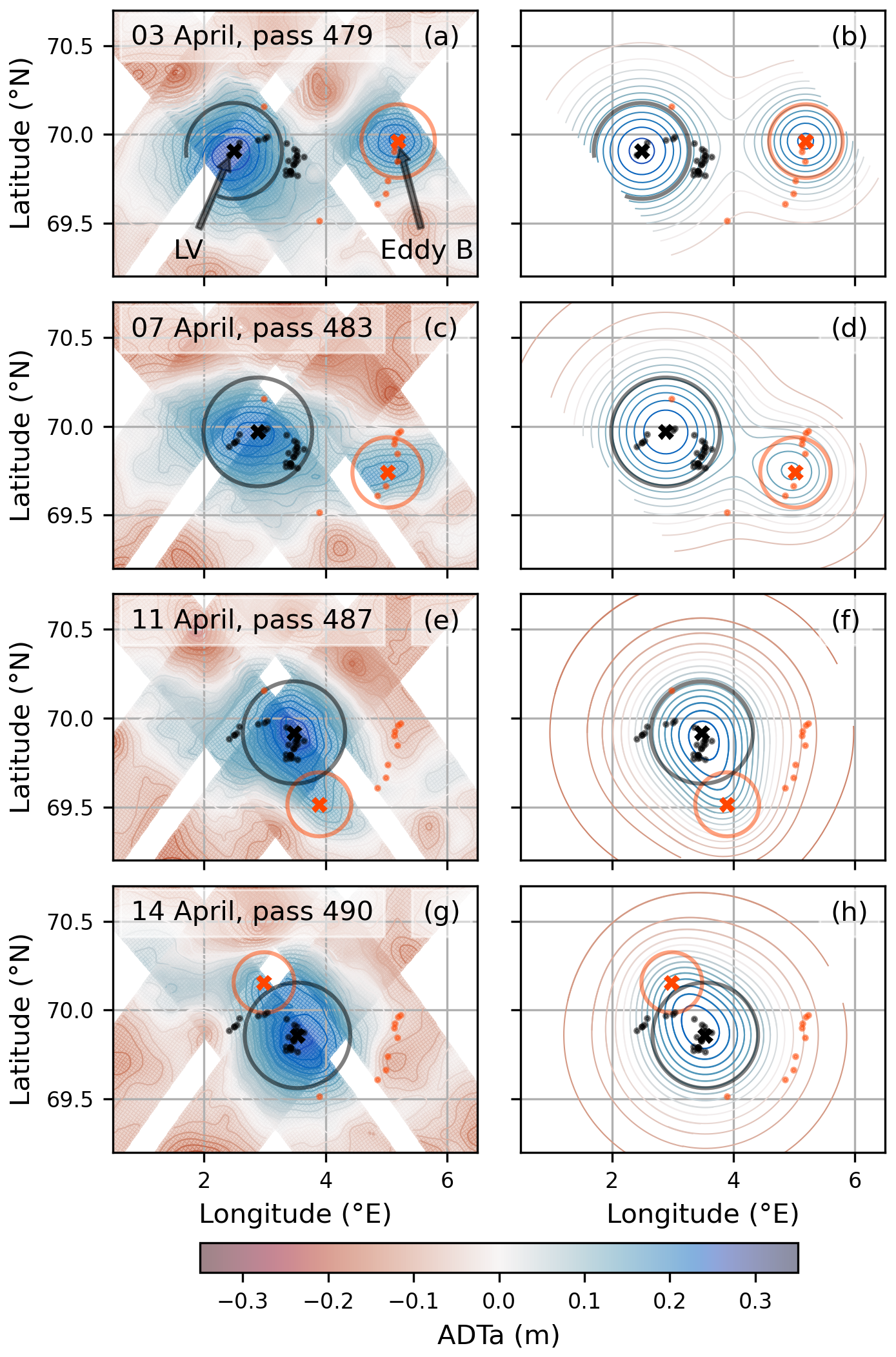
Figure 8 Maps of (first column) SWOT ADTa and (second column) reconstructed fields from Gaussian fits of the LV and eddy B on selected dates in April 2023. Dates: (a, b) 3 April, (c, d) 7 April, (e, f) 11 April, (g, h) 14 April. ADTa contours are shown every 5 cm. The dark-grey dots are LV centre positions (i.e. daily maximum ADT in the study area) from 3 April to 14 April 2023, with the black cross corresponding to the centre position on the date of the panel and the dark-grey circle corresponding to the radius of the Gaussian fit R_LV on that date. Similarly, the orange-red dots are centre positions for eddy B from 3 April to 14 April 2023, with the cross corresponding to the centre on the date of the panel and the coloured orange-red circle corresponding to the radius of the Gaussian fit R_B.

The Gaussian fits to the LV and eddy-B ADT, described in Sect. 2.3 and illustrated in Fig. 8, show the evolution of various properties of both the LV and eddy B from 3 to 25 April (Fig. 9). Prior to the merger, the LV and eddy B have similar amplitudes ($A_{\text{LV}}\simeq A_{\mathrm{B}}\simeq \mathrm{0.25}$ m), but thanks to its smaller radius, eddy B has a significantly stronger vorticity signature, with ${\mathit{\text{Ro}}}^{\text{max}}\simeq -\mathrm{1}$ vs. −0.5 for the LV if one considers cyclogeostrophy (or geostrophy only: ${\mathit{\text{Ro}}}^{\text{max}}\simeq -\mathrm{0.6}$ for eddy B vs. −0.35 for the LV). The error in these Ro estimates computed from the SWOT data is estimated to be 0.07. As the distance between the LV and eddy B decreases, the LV's amplitude and radius increase, while eddy B's amplitude and radius decrease, suggesting that the interaction between the two vortices results in an exchange of mass from eddy B to the LV. The rapid change in these properties should be treated with some caution, however: as eddy B and the LV become more elongated due to their mutual interaction, a circular Gaussian fit becomes less representative. The absorption of eddy B by the LV, and potential ejection of a low-PV parcel from the LV, could also explain the transitional increase in the LV radius (R_LV) observed between 15–20 April, indicating the final stage of the merger. Eddy B's amplitude slowly decreases from 3 April as the two approach each other, but then it drops more rapidly from 7 April onwards as the distance between the LV and eddy B becomes smaller than approximately 80 km, testifying to a stronger interaction between them. The merging process seems to lead to the dissipation of eddy B despite an apparently more dynamical initial Rossby number at the surface (Fig. 9c and Fig. 7). In terms of Rossby number, eddy B quickly loses its strong signature as the interaction with the LV begins, even before the actual merger with the LV core. It is also worth noting that the LV's cyclogeostrophic Rossby number seems to increase in absolute value from about −0.4 to −0.5 between 3–23 April.

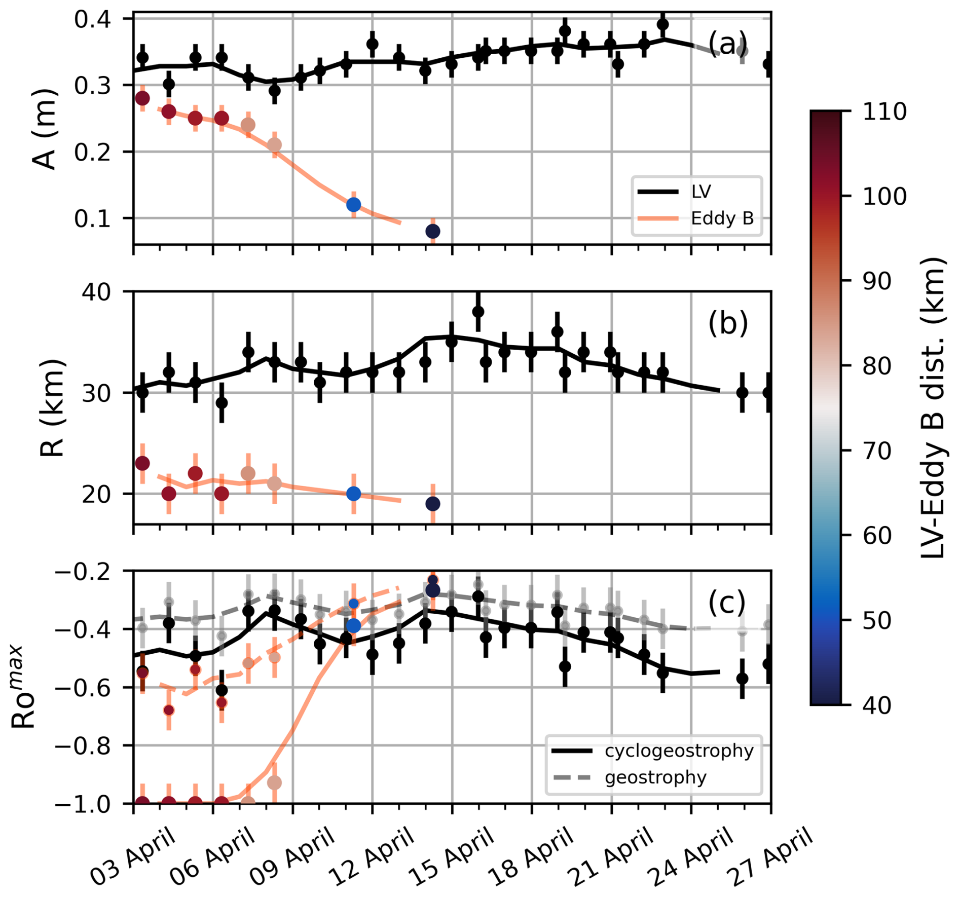
Figure 9 Temporal evolution of properties detected by SWOT with error bars during the April merger event between the LV and eddy B: (a) amplitude, (b) radius from the Gaussian fitting, and (c) maximum Rossby number Ro^max at the LV or eddy-B centre. In all panels, dark-grey dots show values for the LV, with a solid black line showing the 3 d rolling average, and coloured dots show values for eddy B, with a solid orange-red line showing the 3 d rolling average. The colour of the dots represents the distance between the centre positions of the LV and eddy B. In (c), the paler dashed lines and light-grey dots (for the LV) and the dashed orange-red line and smaller coloured dots (for eddy B) show geostrophic estimates, whereas the darker solid line, dark-grey dots, solid orange-red line, and larger coloured dots show cyclogeostrophic estimates (see Sect. 2.3).

3.4 Probable merger event in March

Although the glider passed through eddy B on 14 April and reached the LV core on 15 April, eddy B had not yet reached the LV core by 15 April: the glider was moving faster than the eddy was merging. Hence, the core profiles during realisation 3 are actually profiles from just before eddy B merged in. The LV core is already more stratified than during realisation 1, with warmer temperatures near the surface and a much wider range in density than in realisation 1 (Fig. 5). It has been previously reported that, during winters, a weakened PV gradient in the upper part of the LV between the core and the waters outside the LV reduces the dynamical barrier and facilitates the intrusion of warm waters from the vortex rim (Bosse et al., 2019). While one could speculate that the core and outer temperatures of realisation 1 (Fig. 5a and d) might mix laterally to generate the core temperatures of realisation 3 (and similarly for PV, Fig. 5c and f), the salinity in the core in realisation 3 is fresher than both the core and outer salinities of realisation 1 and thus cannot be formed from a mixture of the two. This strongly suggests that another water mass has contributed to the evolution of the core structure. We speculate that another eddy (eddy A) has already merged into the LV in March for the following reasons:

• From 14 March (when the LV core was observed at the end of realisation 1) to 15 April (when the LV core was observed at the end of realisation 3), the average net surface heat flux over the mean position of the LV was −107 W m⁻² (Fig. 3a). A negative surface heat flux cannot explain an increase in temperature in the LV core, and so there must have been another source of warmer water.

• Similarly, the average net surface freshwater flux from 14 March to 15 April was $-\mathrm{6.1}\times {\mathrm{10}}^{-\mathrm{6}}$ $\mathrm{kg}{\mathrm{m}}^{-\mathrm{2}}{\mathrm{s}}^{-\mathrm{1}}$ (i.e. net evaporation) (Fig. 3b). The core profile for realisation 3 is fresher than the profile for realisation 1 (Fig. 5), which cannot be explained by a negative freshwater flux or, as above, by the intrusion of more saline waters from the vortex rim.

• The META3.2 product shows another distinct eddy (eddy A) approaching the LV earlier in the year (thick blue track in Fig. 2). This track runs from 17 February to 12 March, ending close to the average position of the LV; thus, it may have merged into the LV.

• The LV's azimuthal velocity increased considerably between realisation 1 and realisation 3, from 0.4(±0.05) to 0.6(±0.07) m s⁻¹ (Fig. 4g and h). This kind of “spin-up” is an expected outcome of an eddy merger (Trodahl et al., 2020).

• Finally, the LV appears to have ejected a parcel of low-PV water, seen in Fig. 4q, between approximately 400–800 m depth and 35–60 km from the centre of the LV. Note that this parcel of low-PV water is almost invisible in Fig. B3 because its density range is extremely small. This agrees with the findings of Trodahl et al. (2020), who reported that some low-PV fluid was expelled from the LV during merging events in their modelling study. Moreover, Bosse et al. (2019) used RAFOS float trajectories between 300–800 m to document the Lagrangian coherence of the LV core – except during particular events where several floats were expelled at the same time, consistent with water parcels being expelled from the LV. However, the low-PV parcel seen in realisation 3 was observed by the glider several days before eddy B merged into the LV. Thus, we speculate that this parcel of water may have been ejected during an earlier merger.

Since we lack both in situ observations and the high-resolution SWOT altimetry during this period, we cannot be certain that eddy A merged into the LV between realisation 1 and realisation 3. However, it seems to be the most plausible explanation for the changes in water properties in the LV core, and we will henceforth refer to this as the “probable merger event in March”.

3.5 Impact of the April merging event

To assess the properties of eddy B, observed in April, we use a simple definition to distinguish it from surrounding waters: water with temperatures which are at least 0.2 °C warmer than the temperature of the LV core at the same depth are taken to be within eddy B. This is shown as an orange-red contour in Fig. 4. The properties of eddy B are calculated as an average in each depth bin over the waters enclosed by this contour and are shown in orange-red in Fig. 5. By the time of realisation 5 (18–22 April), the LV core profiles to 400 m are similar to those observed in eddy B a week earlier (Fig. 5). Although Trodahl et al. (2020) found that incoming eddies tended to be lighter than the LV and thus stacked on top of it during mergers to create a double-core vertical structure, we do not observe that here. This is because eddy B is not significantly lighter than the LV: the probable merger event in March has already reduced the density of the upper layers of the LV. In the second column of Fig. 4, a magenta contour marks the minimum potential density observed in the LV core during this realisation (σ₀=27.6) and is equivalent to the red contour in Trodahl et al. (2020)'s Fig. 14. The example of an incoming eddy shown in Trodahl et al. (2020)'s Fig. 14 is lighter than the LV to a depth of approximately 600 m, but in realisation 3, eddy B is only lighter than the lightest water in the LV core to a depth of 40 m. Eddy B therefore simply mixes with the LV rather than stacking on top of it, as also happens to eddies of the same density as the LV in the work of Trodahl et al. (2020). However, eddy B's signature in temperature extends to approximately 400 m depth, and thus it is lighter than the LV core at the same depth, as seen by the deepening of the isopycnals in eddy B compared to the LV core (Fig. 4, second column). Water in the LV core is therefore pushed downward during the merger, as seen by the lowered isopycnals in the LV core in realisation 5 compared to in realisation 3 (Fig. 4). We therefore see the vortex intensification and change in relative vorticity as predicted by Trodahl et al. (2020): in realisation 5, after the merger, the LV's vorticity is even more strongly anticyclonic than in realisation 1, reaching $-\mathrm{0.79}(\pm \mathrm{0.19})f$ (Fig. 4o).

As with the probable merger event in March, we consider whether surface forcing could have brought about the changes in the core properties observed in April. It has not been possible to determine this for salinity because the net change in core salinity was extremely small in the period from 15 to 22 April (i.e. between realisations 3 and 5); a net freshening of only 0.002 g kg⁻¹ over the full water column observed. The average net surface freshwater flux was $\mathrm{9.3}\times {\mathrm{10}}^{-\mathrm{6}}$ $\mathrm{kg}{\mathrm{m}}^{-\mathrm{2}}{\mathrm{s}}^{-\mathrm{1}}$, which is also small, but in combination with the eddy merger, lowering of isopycnals, and possible leakage from the area outside the vortex, it was not possible to separate the different effects. The situation is simpler for temperature because both eddy B and the average net surface heat flux acted to warm the LV. However, the average net surface heat flux of 23 W m⁻² is an order of magnitude too small to bring about the observed temperature change in the LV core; hence, the effect of eddy B merging is dominant.

4 Discussion and conclusions

Conservative estimates of the spin-down timescale for the LV (Fer et al., 2018; Bosse et al., 2019) require that such a long-lived vortex must be maintained by sources that energise it. Merging of mesoscale eddies into the LV has been discussed in the literature as a potentially important mechanism; however, observations in support of merging events have been limited to surface signatures from satellite data (e.g. Raj et al., 2015) or indirect deduction (Bosse et al., 2019). Our study, for the first time, presents a relatively coherent evolution of the surface and subsurface structure during a merging event by combining in situ glider observations with SWOT satellite altimetry data.

The observed merging process closely resembles the modelled process described by Trodahl et al. (2020). As observed at the surface by SWOT, eddy B appeared to be more energetic and slightly smaller than the LV. As the incoming eddy approaches the LV and the two begin to interact, eddy B gradually elongates and becomes attached to the side of the LV, and the two begin to co-rotate. This scenario also resembles quasi-geostrophic shallow-water numerical simulations (Pavia and Cushman-Roisin, 1990; Yasuda and Flierl, 1997; Von Hardenberg et al., 2000; Carton et al., 2016). Our observations do not have the resolution to show the filamentation described by Trodahl et al. (2020), although the elongation of eddy B does suggest that something of that nature may be occurring. Due to cloud cover, no sea surface temperature or ocean colour image could be used during the merger event to document finer-scale filaments. We do not observe a double-core vertical structure after the merger of eddy B and the LV, but this is not unexpected since the density range of eddy B is similar to the LV's density range prior to the merger. The spin-up of vorticity and eddy kinetic energy is also analogous to the merging process modelled by Trodahl et al. (2020). The clear similarities between the modelled and observed process demonstrates that high-resolution models offer complementary insights to better understand details of such eddy processes. However, eddy–eddy interaction remains a complex problem vastly dependent on the initial conditions of the eddies (e.g. PV signature and their vertical structure). Model evaluation crucially relies on our capacity to observe such events.

During the observed period, merging eddies were the dominant process affecting the evolution of the LV. While lateral mixing between the vortex core and the outer rim may also have been a factor, it is clear that, with regard to the heat and salt budgets of the LV core, vertical 1D processes due to atmospheric forcing were greatly outweighed by the eddy merger events. In particular, the merger with eddy A in March substantially altered the water mass properties of the LV, a process continued by the merger with eddy B in April. The influx of warm waters, spin-up of eddy kinetic energy and increasingly anticyclonic vorticity (Fig. 4) will contribute to the longevity of the LV. However, these observations are from a fairly brief period. We observed one merging event clearly and inferred another in the time span of 2 months. This suggests that merging into the LV may be a more common occurrence than found by previous modelling studies, which found three to four merger events per year with no clear seasonal bias (Trodahl et al., 2020), three to four merger events per year but with slightly more mergers occurring during the period February–May and none in November–December (Köhl, 2007), and one to two mergers per year with a distribution skewed towards wintertime (Belonenko et al., 2017). It is possible that merger events in the real ocean are more common than modelled, but their average impact on the LV's properties may be smaller than modelled, as hinted at by the differing impacts of the two merger events discussed here. Longer-term (over several years) in situ observations are still needed to study the evolution of the LV's properties, rate of merger events and possible seasonality in merger events and to quantify the relative importance of wintertime convection vs. merging (Ivanov and Korablev, 1995a, b; Köhl, 2007; de Marez et al., 2021), as well as the role of surface forcing and low-PV parcel ejection from the vortex core (Bosse et al., 2019).

The depth of wintertime convection in the LV can vary greatly, from a few hundred metres in the years observed by Yu et al. (2017) and Bosse et al. (2019) to the more than 1000 m observed by Søiland and Rossby (2013) and Søiland et al. (2016) and seen in the present study. It is not known how representative the characteristics of the eddy merger reported here would be for differing starting conditions such as differing mixed-layer depths or an initial LV which already contains vertically stacked cores. Future observations incorporating biogeochemistry would also be of interest. Deep winter mixing in the LV will increase the vertical flux of nutrients and the depth of oxygen-rich waters, creating conditions which might enhance biological activity in spring. However, deep mixed layers below the euphotic depth inhibit phytoplankton growth: for example, Hansen et al. (2010) found that the onset of spring phytoplankton blooms was delayed by an average of 2 weeks in the deep mixed layers of anticyclonic eddies in the Norwegian Sea. Merging into the LV might enhance the phytoplankton growth in such an eddy through increased nutrient availability or suppress it through deepening the mixed-layer depth. Moreover, if merger events occur more frequently than previously believed, the phytoplankton community in the LV will likely be affected by repeated injections of different water masses carrying different phytoplankton with them.

The new SWOT satellite during its Cal/Val phase provided a truly unique dataset able to document the dynamics of a merger with the LV in the Norwegian Sea. Without the wide swaths and higher resolution (compared to conventional satellite altimetry) of the SWOT data, our analysis would have been impossible. However, in order to fully understand the complex eddy–eddy interactions at play, the surface signature is not sufficient, and the deep PV signature and circulations are important parameters to consider (Verron and Valcke, 1994). Thus, the in situ glider data, which allow for prolonged observations at a relatively high resolution, were also a vital component of this analysis.

Appendix A: Error analysis statistics

The errors in derived variables from glider data (e.g. azimuthal velocity maximum, relative vorticity, Rossby number) are estimated using Monte Carlo simulations (Mooney, 1997), each isolating a specific source of error. We generated 1000 realisations of the variable of interest, calculated from perturbed fields by adding normally distributed error to each measurement point. The error sources analysed are those from the temperature and salinity measurement error, dive-averaged current error, and errors due to the neglect of LV ellipticity.

The accuracy of temperature and salinity measured by a Seaglider's CT sail is typically 0.002 °C and 0.002 on the practical salinity scale (Viglione et al., 2018), and the measurement uncertainty is estimated to be 0.01 °C and 0.01 (Damerell et al., 2016). To err on the side of caution, we used the higher of these estimates.

Uncertainty in DAC measurements has previously been estimated to be 0.01 m s⁻¹ (Todd et al., 2011). We again take a conservative approach by perturbing the meridional and zonal components of the DACs with normally distributed noise with a standard deviation of 0.02 m s⁻¹, twice the uncertainty estimated by Todd et al. (2011). This will generate errors in both the magnitude and direction of the DACs and thus in the glider-estimated centre position, which will generate additional error in the derived variables.

The most complex source of error arises from the assumption of axial symmetry, i.e. the neglect of the LV's ellipticity (Sect. 2.2). Because our derived variables are highly dependent on the radial distance from the glider-estimated centre position to the location of each measurement and DAC estimate, we explored this source of error through manipulation of the radial distances. Within the rotating frame of the LV, the glider will travel approximately along a radial line since it is travelling at 90° to the previous dive's DAC. However, the orientation of this in situ glider transect relative to the ellipse is unknown.

We estimate the ellipticity of the LV by fitting ellipses to the LV ADT data from SWOT in the same way as described in Sect. 2.3 for a circular fit. On 19 of the days in April 2023, we were able to resolve the length of the major and minor axes of an elliptical fit, as well as the radius of a circular fit. Four of these were eliminated for having an un-physically low minor axis length (<10 km), and another six were eliminated because the length of the major axis was less than the radius of the circular fit. This left nine instances. We do not include additional months to increase the number of instances because a month with a merger event (such as April 2023) is the most representative of the situation we investigate here.

We then carried out two Monte Carlo simulations. In the first simulation, we assumed that the glider's transect was aligned with the minor axis of the ellipse. A normal distribution was fitted to the nine observed axis ratios (circular radius/minor axis length, mean of 1.16, standard deviation of 0.14), and 1000 realisations were run using radial distance scaling factors sampled from this distribution. For each simulation, a single scaling factor was applied uniformly to all radial distances. In the second Monte Carlo simulation, we assumed alignment with the major axis and thus fitted a normal distribution to the nine observed axis ratios (circular radius/major axis length, mean of 0.82, standard deviation of 0.13), from which we again ran 1000 realisations.

Note that this approach will tend to overestimate the errors because we only considered the two extremes; i.e. the glider's transect was aligned with the major axis or with the minor axis of the ellipse. It is highly likely that the glider sampled somewhere in between, which would give scaling factors closer to 1 and thus smaller errors in the derived variables.

Results from the error analysis are given in Tables A1 and A2, showing how the minimum vorticity (shown as Rossby number, $\mathit{\text{Ro}}=\mathit{\zeta }/f$) and maximum azimuthal velocity are affected by errors introduced by the CT sail measurement uncertainty, the DAC uncertainty, and the assumption of axial symmetry. Values are given for the mean perturbed value μ, the standard deviation of the perturbed values σ, and the 95 % confidence interval (CI). Since the distributions of the derived variables calculated in the Monte Carlo simulations were approximately normal, the 95 % confidence interval for each derived variable was simply taken to be the range between the 2.5th and 97.5th percentiles of those distributions.

Table A1 Error estimates for Ro due to perturbations of CT sail measurement uncertainty (0.01 °C and 0.01 on the practical salinity scale), DAC measurement uncertainty (2 cm s⁻¹), and the assumption that the glider sampling line was aligned with either the minor or major axis of the elliptical LV. The largest error for each realisation is given in bold.

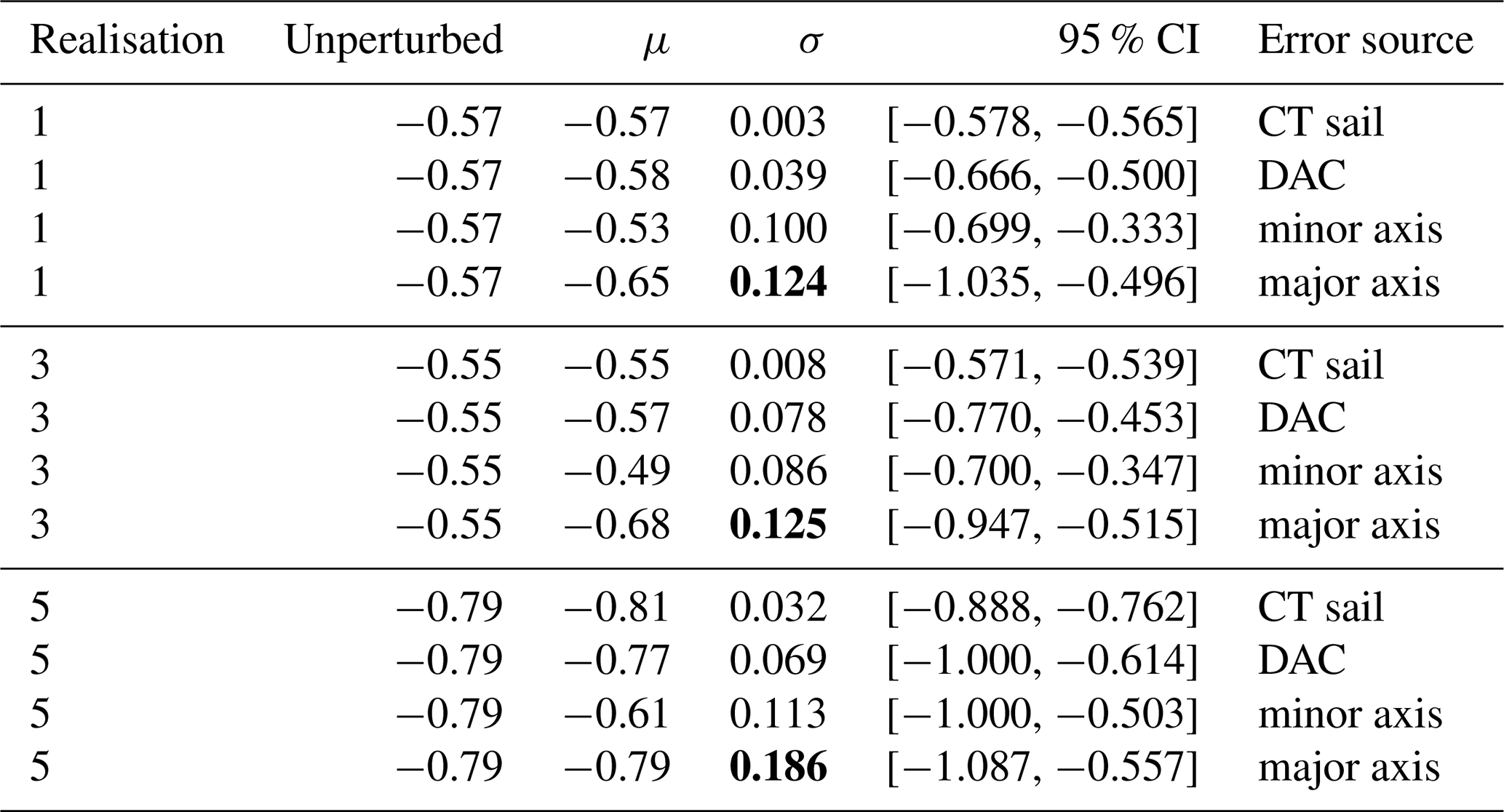
Table A2 Error estimates for maximum azimuthal velocity (in m s⁻¹) due to perturbations of CT sail measurement uncertainty (0.01 °C and 0.01 on the practical salinity scale), DAC measurement uncertainty (2 cm s⁻¹), and the assumption that the glider sampling line was aligned with either the minor or major axis of the elliptical LV. The largest error for each realisation is given in bold.

Appendix B: Additional figures

Here, we present additional figures that could help interpret the observations. Figure B1 shows the glider profiles before optimal interpolation. Figure B2 shows Θ–S_A diagrams for vortex realisations 1, 3, and 5 using all of the data instead of just the average profiles shown in Fig. 5g and h. Figure B3 shows the same panels as Fig. 4, using density as the vertical axis instead of depth.

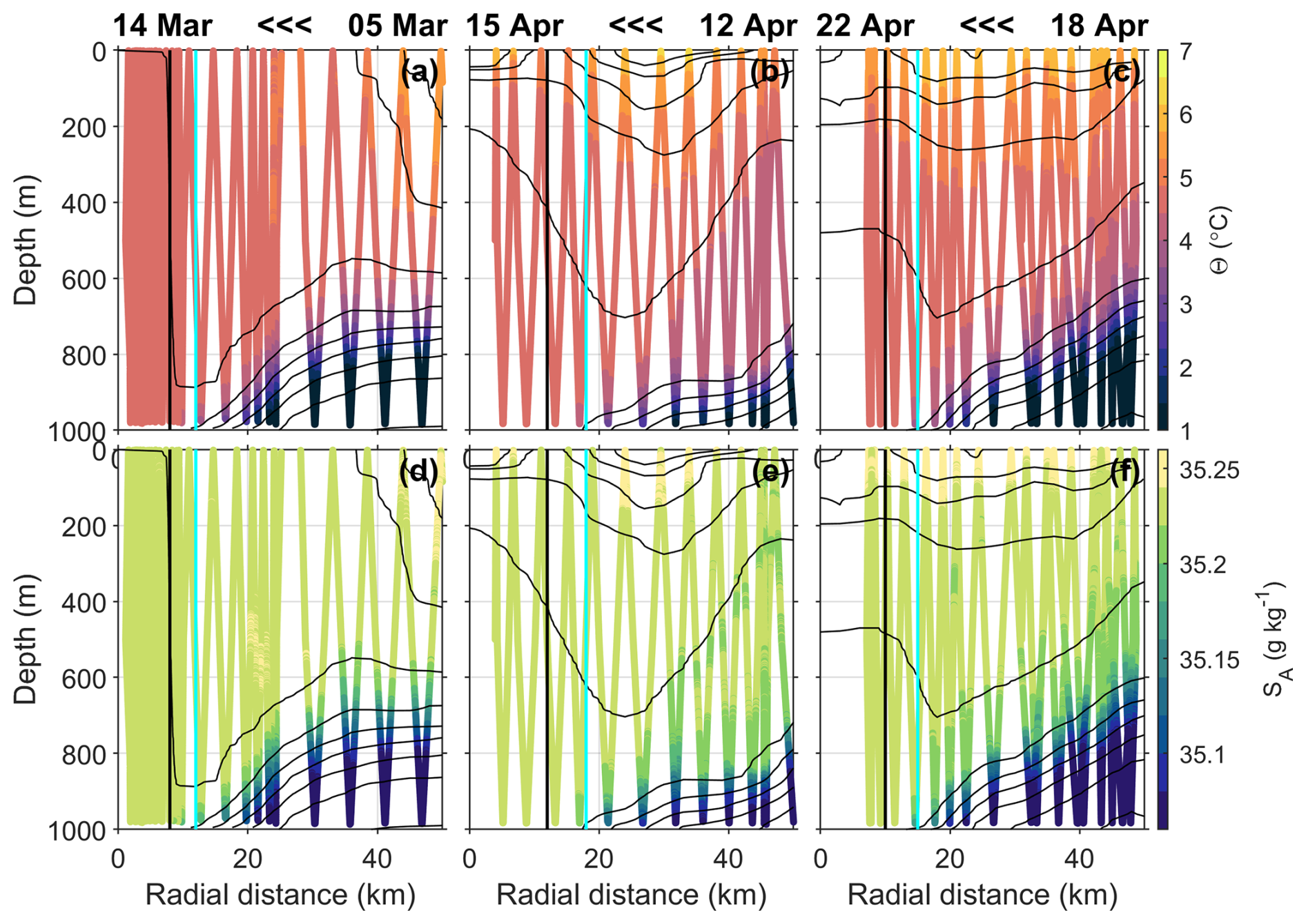
Figure B1 In situ data from the glider before the optimal interpolation described in Sect. 2.2. The first column shows vortex realisation 1 between 5–14 March, the second column shows realisation 3 between 12–15 April, and the third column shows realisation 5 between 18–22 April. Note that, because the glider is travelling from outside the LV towards the centre of the LV in each of these realisations, the left-hand side of each panel is later in terms of date than the right-hand side, as indicated by the labels at the top of each column. (a–c) Temperature and (d–f) salinity. Black contours in all panels show the potential density anomaly (σ₀) every 0.04 from 27.6 to 28.0 kg m⁻³. Vertical cyan lines in all panels show the radius of the core R_c. Vertical black lines show $\mathrm{2}/\mathrm{3}{R}_{\mathrm{c}}$.

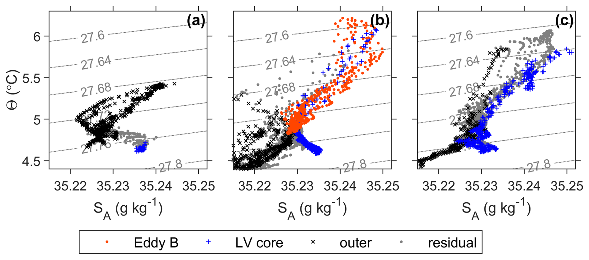
Figure B2 Θ–S_A diagrams for (a) realisation 1, (b) realisation 3, and (c) realisation 5, with those values in the LV core (radial distances $\le \mathrm{2}/\mathrm{3}{R}_{\mathrm{c}}$) shown as blue crosses, the values outside the LV (3R_c to 5R_c) shown as black × symbols, values in eddy B shown as orange-red dots and the residual (i.e. data points which fall into none of these categories) shown as grey dots.

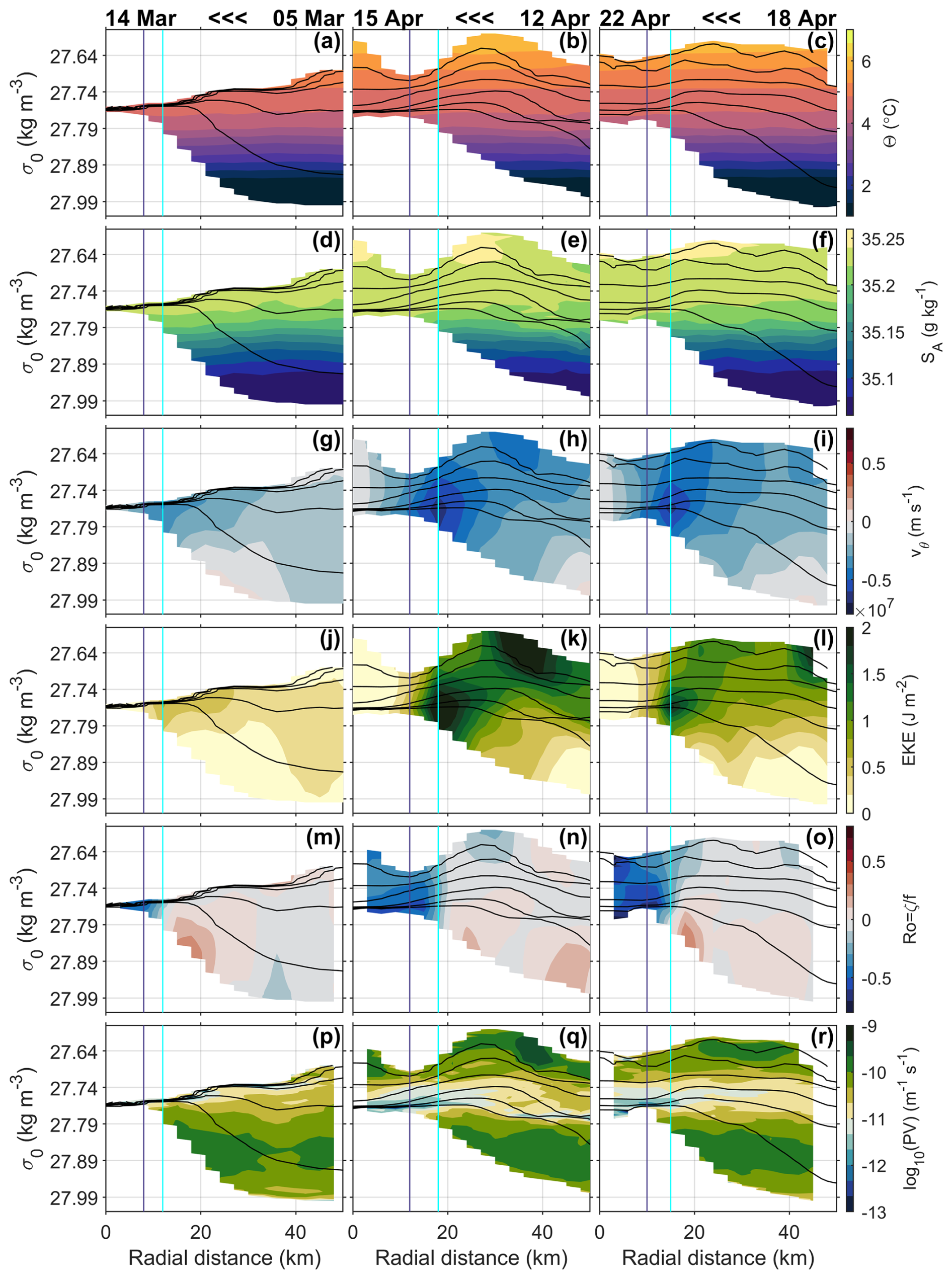
Figure B3 As in Fig. 4 but against density instead of depth. Black contours in all panels are depth contours at depths of 50, 100, 200, 400, 600, and 800 m, except in column 1, which does not show the 50 m contour because of the minimal density change between the surface and 100 m. Note that the y axis scale in all panels is expanded by a factor of 2 between densities of 27.74–27.99 kg m⁻³.