Satellite-derived steric height in the Southern Ocean: trends, variability, and climate drivers

The Southern Ocean circulation plays a central role in regulating the global ocean overturning, ventilating the deep ocean, and driving sea level rise by delivering heat to Antarctic ice shelves. Understanding heat and freshwater content in this region is key to monitoring these global processes and identifying multi-year changes; however, in situ observations are limited and often do not offer the spatial or temporal consistency needed to study long-term variability. Perturbations in steric height can reveal changes in oceanic heat and freshwater content inasmuch as they impact the density of the water column. Here, we show for the first time that the monthly steric height anomaly of the Southern Ocean south of 50° S can be assessed using satellite altimetry and GRACE gravimetry data from 2002 to 2018. Steric height anomalies are validated against in situ Argo float and conductivity–temperature–depth (CTD) data from tagged elephant seals. We find good agreement north of 65° S, but there is increasing uncertainty towards the Antarctic continental shelf due to insufficient validation data, the leakage error, and anti-aliasing in GRACE. The Southern Ocean steric height anomalies capture the expected seasonal cycle of low (high) steric height in winter (summer) and show regionally variable trends during 2002–2018. We find that the variability in steric height is driven predominantly by anomalies in surface heat and freshwater content associated with positive and negative phases of the two major modes of Southern Hemisphere climate variability (the El Niño–Southern Oscillation and Southern Annular Mode). This steric height dataset provides a uniquely comprehensive insight into density anomalies and presents opportunities for further analysis of heat and freshwater fluxes, changes in stratification, or convective regimes across the Southern Ocean.

1 Introduction

The water masses of the Southern Ocean are an essential component of the global thermohaline circulation, connecting the world's oceans and feeding ventilated surface waters into the abyssal ocean (Rintoul, 2018; Morrison et al., 2021). Recent weakening of the overturning circulation (Gunn et al., 2023; Li et al., 2023; Dima et al., 2021) and unprecedented reductions in sea ice (Parkinson, 2019; Haumann et al., 2020; Purich and Doddridge, 2023) have stressed our need to understand the thermohaline characteristics of the Southern Ocean. Reliable, enduring, and comprehensive methods are required to monitor global changes in ocean circulation and assess how heat and freshwater content is responding to climate drivers on multi-year timescales (Null et al., 2023).

The remoteness and hostility of the Southern Ocean impede the collection of high-quality observations, and inter-model variability for key processes such as deep-water formation remains high (Heuzé, 2021). Despite improvements in the quality, frequency, and distribution of oceanographic observations, coverage remains poor, particularly in winter months and permanently ice-covered areas (Smith et al., 2020). Improved coverage and quality of satellite data over the past decade have begun to fill this gap. We are now able to observe the sea surface height (SSH) of the Southern Ocean, including the marginal ice zone (Armitage et al., 2018; Naveira Garabato et al., 2019; Auger et al., 2022), and more accurately measure sea ice concentration throughout the year (e.g. Eayrs et al., 2019; Parkinson, 2019; Kacimi and Kwok, 2020). Developments in gravimetry, specifically in the GRACE experiment, provide comprehensive observations of mass transports throughout the global ocean and show increasing accuracy within small ocean basins, near coastlines, and in polar regions (Dobslaw et al., 2020; Dobslaw et al., 2017; Shihora et al., 2022). Here, we exploit these recent improvements in satellite technology to calculate steric height in the Southern Ocean, a metric related to water column density, from which information on oceanic temperature and salinity changes can be inferred.

Steric height is the contribution to SSH from changes in the density of the water column. Higher steric height values indicate a less dense (fresher and/or warmer) water column, while lower values denote a denser (colder and/or more saline) water column. Steric height derived from satellite data agrees closely with in situ observations in both global (Purkey et al., 2014; Feng and Zhong, 2015) and regional (Armitage et al., 2016; Karimi et al., 2022; Raj et al., 2020) studies and can reveal large-scale information about water column structure such as mixed layer depth (Gelderloos et al., 2013) and freshwater content (Lin et al., 2023; Armitage et al., 2016). Changes in these properties across the Southern Ocean are currently under scrutiny due to their impact on the global ocean and uncertain relationship to climate change, yet few studies have attempted to explore these changes via steric height. Rye et al. (2014) use a combination of satellite SSH and model output to compute the steric contribution to sea level rise around the Antarctic continent, finding a relative increase in SSH on the shelf compared to the rest of the Southern Ocean between 1992 and 2011. They attribute this to the freshening of the surface waters from increased ice sheet melt rates and warmer waters at depth, which dominate over local increases in ocean mass. Kolbe et al. (2021), using a model-based approach, found an overall decrease in the steric height of the Southern Ocean waters between 2008 and 2017 due to an increase in surface salinity. We aim to provide fresh insight into this conversation with a comprehensive and updated picture of the Southern Ocean steric height, using a purely observation-based approach.

Using remote sensing methods to approximate steric height is more challenging at high latitudes than in lower-latitude oceans. Altimetric measurements of the sea surface are inhibited by sea ice, and the use of retracking algorithms to reconstruct SSH from ocean leads can result in discontinuities at the ice zone margin (Bamber and Kwok, 2004; Tilling et al., 2018). Armitage et al. (2016) used bespoke processing methods to compute the SSH of both the ice-covered and ice-free Arctic Ocean, using data from multiple satellites. Biases between satellite eras and sea ice zones were identified and minimised, resulting in a coherent, multi-decadal SSH dataset from which steric height was estimated. The steric height was validated against Argo float data and demonstrated the feasibility of the method used herein. The Southern Ocean presents a more complex problem than the Arctic Ocean; strong winds and intense ocean currents drive complex upwelling and downwelling patterns and rough sea surface conditions that can affect the accuracy of satellite observations (Kacimi and Kwok, 2020; Kuo et al., 2008). Satellite research in Antarctica is relatively immature compared to the Arctic, and the nature of Antarctic sea ice and its impact on satellite observations is not as well understood (Gabarró et al., 2023).

In this article, we combine a multi-satellite SSH dataset spanning both the ice-covered and ice-free Southern Ocean with gravimetry data from GRACE to reveal steric height anomalies south of 50° S during 2002–2018 (Fig. 1). We validate the steric height anomaly dataset against in situ geopotential height computed from Argo floats and tagged elephant seal CTD data and qualitatively assess regional uncertainties, tracing such uncertainties back to specific satellite processing methods. We explore the trends and variability in steric height, drawing links to indices of the two major modes of Southern Hemisphere climate variability (the El Niño–Southern Oscillation and Southern Annular Mode) to explain inter-annual fluctuations in steric height. Finally, we discuss how our findings compare to build upon the existing knowledge base and describe the potential applications of our method.

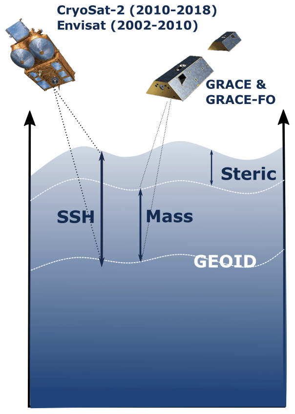
Figure 1 Schematic showing the contribution of barystatic height and steric height to total sea surface height (SSH). Barystatic height is the mass component and is measured using the GRACE twin satellites, which evaluate gravitational field strength. Steric height is the density component and is estimated by the altimeters on CryoSat-2 and Envisat.

2 Data and methods

2.1 Dynamic ocean topography

The dynamic ocean topography (DOT) has been calculated using a pre-processed satellite altimetry product from the combined SSH from Envisat (July 2002 to March 2012) and CryoSat-2 (April 2010 to July 2018). Dragomir (2023) gridded along-track data from both satellite missions onto a 1° longitude × 0.5° latitude grid and merged the data from CryoSat-2 and Envisat. The overlap between the satellites' operating periods was used to calculate and remove the offset between the two, which varies from 1–2 cm (Armitage et al., 2016). The resulting monthly SSH was then referenced against the GOCO05c geoid (Pail et al., 2016) to give DOT and smoothed using a 300 km Gaussian filter. We do not perform any further processing on the DOT.

2.2 Barystatic height

Barystatic height is the mass-only component of SSH (i.e. excluding steric effects). To estimate changes in barystatic height, we use the GRACE/GRACE-FO RL06 Mascon Solutions (version 2) from the Centre for Space Research (Save, 2020; Save et al., 2016). The GRACE mascons are gridded monthly means of the liquid water equivalent in metres of mass (i.e. barystatic) change relative to a baseline average from 2004 to 2009. We re-sampled the mascon data onto the DOT grid using linear interpolation. Where data were missing in time, we linearly interpolated up to 2 months forward or back from the last or next month with an available data point. Missing data more than 2 months apart from an available data point are left as null values. There is a prominent data gap from July 2017 to May 2018 between the final recording from GRACE and the first recording from GRACE-FO.

The GRACE mascon solutions used here have been processed into monthly values on a 0.25° grid; however, they represent underlying data of a roughly 300 km spatial resolution that have been temporally accumulated over 7–30 d (Save, 2020). The impact of this processing could be significant in the dynamic Southern Ocean and Antarctic environment, and we explore this in Sect. 4.2.1.

2.3 Steric height

We compute the steric height anomaly (SHA) by subtracting the barystatic height anomaly (BHA) from the sea surface height anomaly (SSHA). Since changes in sea surface height arise from variations in either mass (barystatic) or density (steric), this leaves only the density contribution, equivalent to SHA:

$$\begin{array}{}\text{(1)}& \mathrm{SHA}=\mathrm{SSHA}-\mathrm{BHA}.\end{array}$$

Since DOT is SSH relative to the geoid, a mean reference surface, the DOT anomaly (DOTA), is equivalent to the SSHA. We compute the DOT anomaly by subtracting the mean DOT over the dataset period (July 2002 to June 2018). The GRACE mascons provide the barystatic height as an anomaly relative to a baseline of 2004 to 2009; however, we re-calculate the anomaly relative to the period July 2002 to June 2018 for consistency with the DOT data.

2.4 Geopotential height

We validate the satellite-derived SHA dataset against the geopotential height (GPH) computed from in situ hydrographic profiles from Argo floats (Riser et al., 2018) and seal-mounted CTD instruments (Roquet et al., 2014). One profile consists of a series of concurrent temperature, salinity, and pressure observations corresponding to a single time, latitude, and longitude. Each observation is marked with a quality flag, where “1” indicates good-quality data.

We calculate GPH relative to 500 dbar to maximise the quantity and geographical distribution of profiles available for validation; profiles from tagged elephant seals constitute a large proportion of data on the shelf, and while Argo floats often go to 2000 dbar, elephant seals rarely dive below 500 dbar. Empirical and theoretical studies have shown that the circulation in the Southern Ocean follows an equivalent barotropic mode; thus, the thermohaline properties within the surface 500 m are highly correlated with those at depth (Meijers et al., 2011; Killworth and Hughes, 2002). Indeed, we find a strongly significant correlation of 0.98 between GPH relative to 500 and 1800 dbar in a subsample of Argo data across the Southern Ocean (not shown).

Starting with all profiles south of 50° S, we discard any profiles containing fewer than 2 good-quality observations. We then discard profiles with a maximum pressure of less than 500 dbar and a minimum pressure of greater than 25 dbar. The limit of 25 dbar is sufficiently shallow to capture changes in GPH close to the surface and sufficiently deep to retain data from Argo floats trapped beneath ice, in the case that they cannot reach the surface but continue to profile at depth. In order to retain winter profiles, we do not omit under-ice profiles or correct their locations (the co-ordinates of under-ice profiles are approximated by linearly interpolating between the points before and after the float became trapped below the surface). This down-selection yields a total of 289 441 valid profiles with good coverage of the Southern Ocean over our study period, though with a marked increase in quantity after 2008 (Fig. S1 in the Supplement).

The GPH is computed for each of the remaining profiles according to the equation below, where density ρ has been calculated using the Gibbs seawater (GSW) density function (McDougall and Barker, 2011) using the adjusted pressure, temperature, and salinity fields from the Argo float and seal profiles and reference density ρ_ref is the density at 35 psu and 0 °C for each vertical level P in the adjusted pressure.

$$\begin{array}{}\text{(2)}& {\displaystyle }\mathrm{GPH}={\int }_{\mathrm{0}}^{p_{\mathrm{500}}}{\displaystyle \frac{\mathrm{1}}{\mathit{\rho }}}-{\displaystyle \frac{\mathrm{1}}{{\mathit{\rho }}_{\mathrm{ref}}}}\mathrm{d}p,\text{(3)}& {\displaystyle }{\mathit{\rho }}_{\mathrm{ref}}=\mathit{\rho }(\mathrm{35}\mathrm{psu},\mathrm{0}\mathit{°}\mathrm{C},P).\end{array}$$

To facilitate the comparison against the satellite-derived steric height, our entire GPH dataset is mapped onto the SHA grid by computing the monthly mean of all GPH profiles falling into each cell. We then compute the geopotential height anomaly (GPHA) for each grid square by subtracting the mean GPH from July 2002 to June 2018 for consistency with the DOT and GRACE (and therefore SHA) anomalies. This method of gridding provides a dataset with a scale that is broadly comparable to that of the SHA.

2.5 Geographic nomenclature

For clarity in this study, we present the different regions of interest within the Southern Ocean in Fig. 2. To discuss basin-wide results, we divide the Southern Ocean into four sectors: the South Atlantic Ocean, the South Indian Ocean, the Australian–Antarctic Basin, and the South Pacific Ocean. The basins are further divided into seas, within which local steric processes can be more easily described. The dynamics of each basin and sea are distinct from one another and result in large regional, seasonal, and inter-annual differences in sea ice cover, heat, and freshwater fluxes.

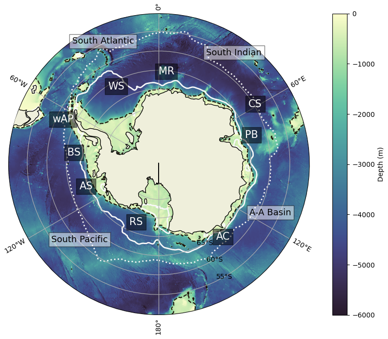
Figure 2 Bathymetric map of the Southern Ocean showing the major ocean basins (South Atlantic, South Indian, Australian–Antarctic (A–A), and South Pacific) and the smaller regions of interest (Weddell Sea (WS), Maud Rise (MR), Prydz Bay (PB), Cooperation Sea (CS), Adélie Coast (AC), Ross Sea (RS), Amundsen Sea (AS), Bellingshausen Sea (BS), and western Antarctic Peninsula (wAP)). The extent of the seasonal ice zone (dotted white marks), the area where the sea ice concentration (SIC) exceeds 0.15 on average in August, and the extent of the permanent ice zone (solid white marks), where SIC is above 0.15 at least 95 % of the time are shown. Also marked is the −1000 m isobath (dashed black). Bathymetry data were obtained from GEBCO (see “Data availability”) and sea ice concentration from NSIDC (Meier, 2024).

3 Results

3.1 Validation of SHA against observations

We compare the average monthly SHA against the average monthly GPHA across the whole domain (Fig. 3a, b). Both show a seasonal cycle with an amplitude of 2.5 cm. The SHA data display a peak in February, during austral summer, coinciding with the minimum sea ice concentration (Fig. 3c), while the GPHA peaks in March. The SHA data reach a minimum in September–October, during the end of austral winter, with the GPHA at its lowest in September. The monthly averages of SHA and GPHA show good agreement to within 0.25 cm for most months, except May, when there is a larger discrepancy of 0.6 cm. This is explored further in Appendix A.

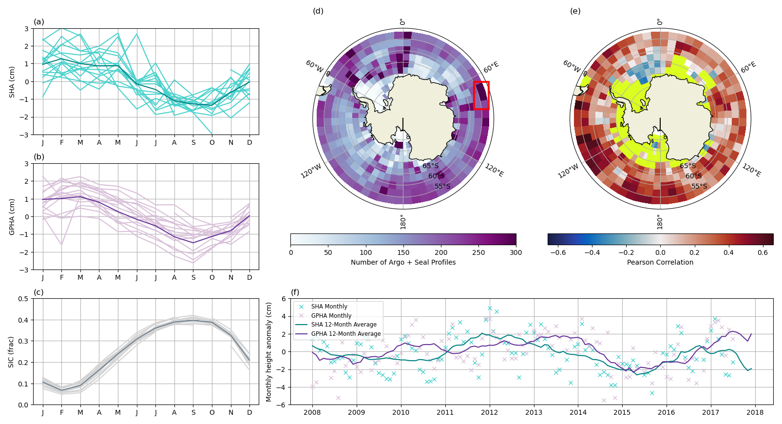
Figure 3 Validation of SHA against GPHA from Argo and seal profiles. (a) The monthly average SHA (darker line) across the entire domain. (b) The monthly average GPHA across the entire domain. (c) The monthly average sea ice concentration (SIC) across the entire domain. Individual years' data are shown as lighter lines in (a), (b), and (c). (d) The total number of profiles recorded within each grid square. The red box outlines the region from which the data in (f) have been taken. (e) The Pearson correlation coefficient between the SHA and GPHA for each grid square. Pixels with less than 36 months of data are masked in yellow. (f) Comparison between the SHA and GPHA time series for the location shown in (d). Monthly measurements are shown with an “x” and the 12-month rolling mean as a solid line.

We next perform a spatial comparison of SHA and GPHA. We coarsen the SHA/GPHA grid by a factor of 6 so that the new grid measures 3° latitude × 6° longitude. We re-calculate the GPHA in the same way as before (see Sect. 2.4), relative to the new grid squares. By coarsening the grid, we increase the amount of data within each cell and decrease the overall resolution such that the profile data are more comparable to the SHA, which is formed from relatively low-resolution satellite data. The total number of profiles recorded within our analysis period for each grid square is shown in Fig. 3d. We compute the Pearson correlation coefficient for the SHA and GPHA time series at each grid square (Fig. 3e). We exclude pixels where there are fewer than 36 non-consecutive months' worth of simultaneous SHA and GPHA data (i.e. over the entire 192-month analysis period, data are available for both SHA and GPHA); based upon analysis of individual grid squares, this achieves a sufficiently high number of degrees of freedom to accurately validate the SHA data while retaining enough grid squares to produce a comprehensive correlation map. The correlation between the SHA and GPHA exceeds 0.25 across 49 % of grid cells shown, rising to 57 % for grid cells north of 65° S. Further south, we find some areas exhibiting good correlation, such as the Bellingshausen Sea (with an average correlation of 0.43) but a swathe of negatively correlated pixels from 30° W to 0°.

While we consider 36 months of data sufficient to compare GPHA and SHA on our coarse correlation map, a higher data density is required for more precise and local comparison. We isolate the data from the grid cells covering the Kerguelen Islands (65 to 80° E, 55 to 50° S), where there is a high density of profile data (Fig. 3d) due to this being a primary site of seal tagging and release (Roquet et al., 2014). Here, multiple profiles are available for each month, permitting a time series of monthly averages to be constructed for this location (rather than relying on a single profile or handful of data points to represent each month, as is the case in other locations with lower data density). Satellite data represent a monthly mean; thus, this improves the validity of the comparison.

The 12-month rolling means of the monthly height anomalies from the satellite-derived SHA and profile-derived GPHA are similar in both shape and magnitude; the SHA and GPHA time series reach a maximum anomaly of 2 cm in 2012 and 2013, respectively, before both falling to a minimum of −2 cm in 2015, then rising again until 2017 (Fig. 3f). The magnitudes differ by up to 2 cm but are usually within 1 cm. This discrepancy does not necessarily arise from the error in SHA alone; it may also reflect any combination of the following: (a) error in the satellite measurements used to compute steric height, (b) incompleteness of the profile data resulting in biases, or (c) limitations of comparing in situ point data to spatially smoothed satellite data over a relatively small area. The amplitude of the seasonal cycle of GPHA in this location can be up to 8 cm, with inter-annual variations of up to 4 cm; therefore, this margin of error in the SHA data is likely to capture changes over multi-month timescales.

Across almost the entire continental shelf, the amount of in situ data are insufficient to perform a validation of SHA via gridded comparison. We use individual float data to validate the SHA in the Ross Sea, where some in situ profiles are available and find a seasonal discrepancy (Appendix A). For the remainder of this study, we present the results in all locations for exploratory analysis and the readers' interest. We interpret and discuss basin-wide changes over inter-annual timescales, which we believe are well served by the present dataset, but suggest that further validation be performed for small-scale studies.

3.2 Steric height trend and variability 2002–2018

We compute the linear trend in SHA from July 2002 to June 2018 (Fig. 4a). The trend is regionally variable but predominantly negative, indicating an increase in water column density across most of the Southern Ocean southwards of 50° S. The South Pacific and South Indian oceans show the strongest negative trends, with maxima of −0.7 and −0.5 cm per year, respectively. There is also a negative steric height trend along the coastline of the Bellingshausen and Amundsen seas and on the shelf in the Weddell Sea. In contrast, the South Atlantic Ocean shows a positive steric height trend, with maxima in the Drake Passage and on the western Antarctic Peninsula (wAP) of up to 1 cm per year. In contrast to other locations along the Antarctic coastline, the Adélie Coast also shows a positive SHA trend and thus a decreasing density. The Australian–Antarctic Basin exhibits patches of both increasing and decreasing steric height, with a stronger positive trend at lower latitudes.

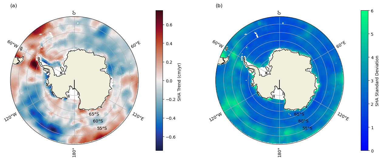
Figure 4 Steric height linear trend (a) and standard deviation (b). Geographical nomenclatures are displayed in Fig. 1. Data quality may vary regionally (please refer to Sect. 3.1 for validation results).

SHA shows the greatest variability in concentrated areas along the coastline of South America and the Antarctic continent, in the Drake Passage, and across the South Pacific Ocean between 50 and 60° S (Fig. 4b). Strong seasonal or inter-annual fluctuations in SHA arise from changes in the density of the entire water column. We expect to see higher variability on the coast since (a) the total volume of water is lower in shallower areas and (b) coastal processes such as freshwater runoff, ice–ocean interactions, and up-/downwelling can result in significant water mass transformations over short periods of time. The South Atlantic Ocean displays low variability, especially within the Weddell gyre, where the density of the water column remains relatively stable over time.

We perform an empirical orthogonal function (EOF) analysis on the SHA dataset (Rieger and Levang, 2024). We retain the seasonal cycle so that its influence on overall variability may be assessed. The spatial components of the first three modes are shown in Fig. 5a, b, and c, along with the winter sea ice maximum extent, −1000 m isobath, and the respective explained variance ratio (EVR). The temporal components of the modes are shown in Fig. 5d, e, and f.

Figure 5 Spatial signatures of mode 1 (a), mode 2 (b), and mode 3 (c) resulting from EOF analysis of SHA. The colour scale is arbitrary but consistent across (a), (b), and (c) and centred at zero. The explained variance ratio (EVR) is shown in the title. The sea ice maximum is demarcated in solid white and the −1000 m isobath in dashed black lines. Temporal signatures of mode 1 (d), mode 2 (e), and mode 3 (f). The scale on the y axis is arbitrary but consistent across (d), (e), and (f) and centred at zero. Data quality may vary regionally (please refer to Sect. 3.1 for validation results).

The first mode, accounting for 23 % of the variability, shows little spatial structure or conformity to the sea ice maxima or −1000 m isobath. It captures a simultaneous rise in steric height across almost the whole domain, strongest in the South Pacific and with a small decrease in the wAP. The temporal component is dominated by an annual fluctuation reflecting steric height changes resulting from the seasonal cycle.

The second mode shows anomalously low steric height in the South Pacific Ocean between 90 and 165° W (referred to hereafter as the southwestern Pacific) and an opposing positive anomaly in the southern Atlantic, on the wAP, and in the South Pacific Ocean between 170° W and 140° E. A weaker positive signal bound by the sea ice maximum exists in the Ross Sea and on the Adélie Coast, contrasting with a weak negative signal within the sea ice maximum in the Cooperation and Weddell seas. The Weddell Sea and Cape Darnley show a negative anomaly landward of the −1000 m isobath. The spatially averaged SHA time series pertaining to the second mode (Fig. 5e) exhibits a seasonal cycle superimposed upon a more dominant low-frequency signal, which oscillates over more than 10 years, suggesting these changes are driven primarily by an inter-annual mode.

Mode 3 accounts for 7 % of the observed variability and, broadly speaking, shows an increase in SHA within the seasonal ice zone (landward of the sea ice maximum) and a decrease at most longitudes outside of the seasonal ice zone. The strongest anomalies exist on the shelf in the Weddell Sea, Prydz Bay, and Ross Sea, all regions where there are large ice shelves, with another hotspot off the shelf in the wAP. Mode 3 remains relatively stable over multi-year timescales until around 2013, when it begins to decrease. Mode 3 loosely reflects the spatial pattern in steric height related to sea ice melt, increasing within the sea ice zone as the density decreases due to the addition of freshwater.

Across all modes, the wAP, the South Pacific, and the Weddell Sea shelf regions show strong variability. We might expect heightened density variability in these regions, particularly when compared to the gyres, due to increased eddy activity, which redistributes water masses of different properties. The EVR of the first 3 modes accounts for 39 % of the variability, suggesting that while seasonal fluctuations and inter-annual climate modes have a major effect, most of the variability is driven by a myriad of independent processes. The higher modes (not shown) display spatial patterns and trends that are more independent of sea ice, bathymetry, and seasonal cycles and may be useful when examining local changes or specific water masses.

3.3 Inter-annual mode composite analysis

To visualise the steric height response to the Southern Oscillation, a major mode of Southern Hemisphere climate variability, we compare composites of the SHA in months with a positive and negative Southern Oscillation Index (SOI). We apply a 1-year filter to the SOI and choose months in which the SOI is greater or less than 1/−1 standard deviation to represent positive/negative SOI years, then take the average of the 1-year filtered SHA within these months for the composite (Fig. 6a).

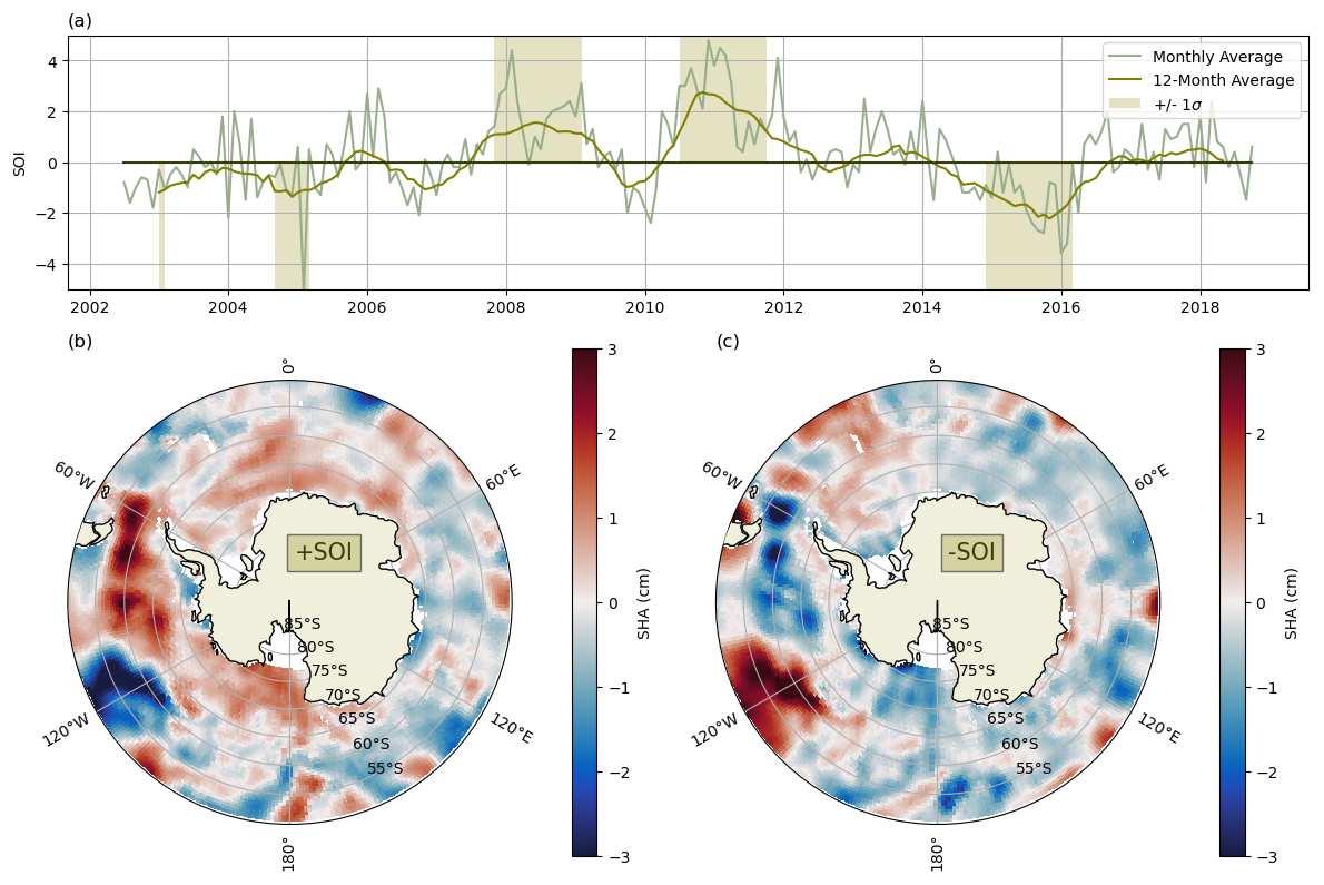
Figure 6 (a) Time series of the Southern Oscillation Index (SOI) smoothed over 12 months. Months showing an SOI greater than 1 standard deviation or less than −1 standard deviation are highlighted in pale green. (b) Composite plot of SHA within months where the SOI is greater than 1 standard deviation. Panel (c) is the same as panel (b), but where the SOI is less than −1 standard deviation. SHA has also been smoothed over 12 months. Data quality may vary regionally (please refer to Sect. 3.1 for validation results).

The SOI is the difference in surface air pressure between Tahiti and Darwin, Australia. Periods of sustained negative (positive) SOI correspond to anomalously warm (cool) temperatures in the eastern tropical Pacific, known as El Niño (La Niña) events (Turner, 2004). The temperature anomalies in the tropical Pacific propagate to the South Pacific via atmospheric Rossby waves (Karoly, 1989), affecting the depth of the Amundsen Sea Low (ASL) (Raphael et al., 2016; Turner et al., 2013). During a La Niña event, the ASL deepens and pulls warm surface water towards West Antarctica (Henley et al., 2015; Holland and Kwok, 2012; Stammerjohn et al., 2008), resulting in a dipole between the South Pacific Ocean and the Bellingshausen and Amundsen seas (Yuan and Martinson, 2001; Kwok and Comiso, 2002).

The SOI composites display a zonally variable response to the Southern Oscillation (Fig. 6b, c). The key feature is the dipole between the South Pacific and wAP, exhibiting a positive SHA in the South Pacific and negative SHA in the wAP during negative SOI phases. The signal in the Ross Sea is coherent with the wAP. Both features show some similarity to the second and third modes identified in our EOF analysis (Sect. 3.4). The SHA in East Antarctica is less affected by the Southern Oscillation than that in West Antarctica, suggesting weaker influence from the Pacific. In the Weddell Sea, there is a weakly positive SHA in an otherwise negative area that appears to follow the export pathway for Antarctic Bottom Water (Morrison et al., 2020). This could suggest changes in dense Weddell Sea water classes in response to SOI fluctuations; however, this is conjectural, and changes of this nature are likely to occur over timescales longer than 1 year. We also see weak opposing signals between the South Indian Ocean and along the coast of East Antarctica, which could indicate bipolar large-scale pressure changes that have not yet been investigated.

The Southern Annular Mode (SAM) is another major mode of variability in the Southern Ocean that is likely to be linked to changes in steric height. However, isolating the SHA response to positive and negative SAM phases is difficult due to the positive trend and increasing amplitude of the SAM index over our study period. To account for this, we apply an 18-month filter and consider months in which the SAM is greater than 2× the standard deviation as positive and months in whcih it is below 0 as negative (Fig. 7a). We show only the composite of SHA corresponding to positive SAM phases since there are too few negative SAM months in the study period.

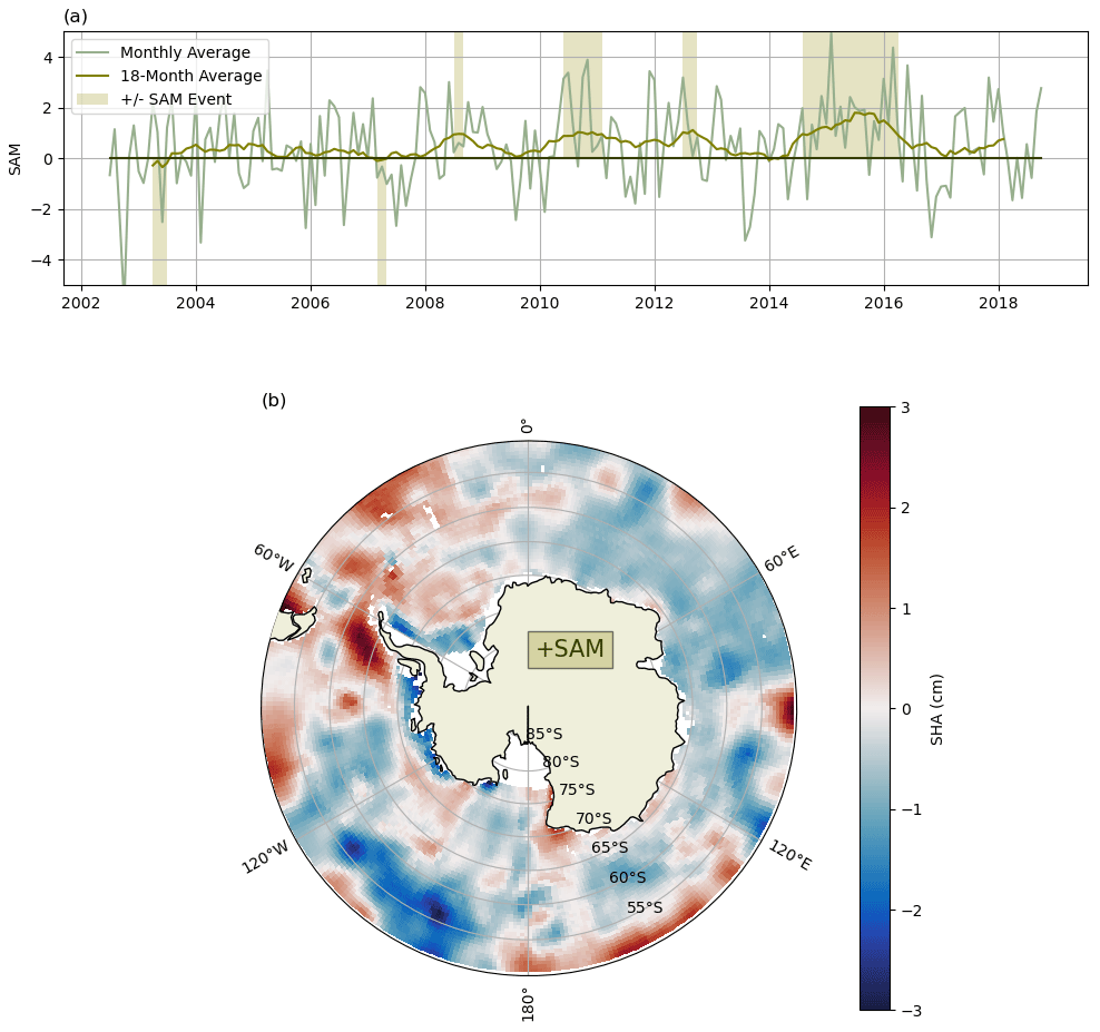
Figure 7 (a) Time series of the Southern Annular Mode (SAM) index smoothed over 18 months. Months in which the SAM index is greater than 2 standard deviations or less than zero are highlighted in pale green. (b) Composite plot of SHA within months in which the SAM index is greater than 2 standard deviations. SHA has also been smoothed over 18 months. Data quality may vary regionally (please refer to Sect. 3.1 for validation results).

The SAM is the primary mode of climate variability in the Southern Ocean and describes the oscillation in the zonally symmetric pressure anomaly in Antarctica relative to the mid-latitudes. A positive SAM (+SAM) index denotes negative Antarctic sea level pressure anomalies and is associated with an intensification and contraction of surface westerly winds towards the pole. Similarly to SOI, we find a regionally variable response in the SHA of the Southern Ocean to the SAM. Close to the continent, +SAM is associated with a strong positive SHA on the wAP and a strong negative SHA on the shelf in the Bellingshausen and Amundsen seas and on the eastern side of the peninsula (Fig. 7b). A moderate negative anomaly dominates the other shelf regions, except for the Adélie Coast and eastern Ross Sea, where the steric height rises in response to +SAM. Farther offshore, the SHA response is predominantly negative; the signal is strongest in the South Pacific, with a weaker and more uniform negative signal in the South Indian Ocean. The Weddell and Scotia seas show patchy positive SHA signals throughout. In general, the spatial patterns in SHA during a +SAM period appear very similar to those associated with the second mode of our EOF analysis. The EOF mode 2 time series (Fig. 5e) also appears to mirror the SAM time series (Fig. 7a), suggesting that changes related to the SAM could be a primary driver of steric height changes in these regions. These results are particularly relevant considering the increasing trend in the SAM; if the SAM continues its tendency towards a more positive phase, the conditions associated with these steric height patterns may intensify.

4 Discussion

4.1 Mechanisms of SHA variability

The trend in SHA between 2002 and 2018 is regionally variable but shows an overall decrease, with large areas of declining steric height across the South Pacific, South Indian, and Ross Sea sectors (Fig. 4a). This is initially surprising, as rising ocean temperatures and increasing freshwater input from sea and land ice might suggest a decrease in density and thus an increase in steric height. The density of the Southern Ocean, particularly at higher latitudes, is predominantly governed by changes in salinity, and the decline in steric height has previously been linked to increased salinity of the upper and intermediate layers (Kolbe et al., 2021). The meridional overturning circulation of the Southern Ocean allows deep, salty water to upwell south of the Antarctic Circumpolar Current (ACC) and supports the northward transport of heat, increasing the density of high-latitude waters (Armour et al., 2016). An amplification of this effect is consistent with the findings from Kolbe et al. (2021) and could underpin the large-scale changes in steric height we observe.

While these mechanisms contribute to the widespread decline in steric height, regional increases are likely to reflect changes in local processes and water properties. The patchy steric height increases in the Australian–Antarctic Basin may reflect the observed freshening of deep waters (Purkey and Johnson, 2013; van Wijk and Rintoul 2014; Purkey et al., 2019). The increasing steric height in the Weddell Sea is likely to be linked to decreasing density from the observed warming and freshening trend, which is possibly driven by a decrease in the denser classes of Antarctic Bottom Water (Meredith et al., 2011; Purkey and Johnson, 2013; Zhou et al., 2023; Strass et al., 2020). Increased ice melt in West Antarctica (Smith et al., 2020), particularly on the peninsula, is likely to explain the increasing SHA on the wAP due to freshening (Ding and Steig, 2013).

We can exploit the similarity between the SHA trend map (Fig. 4a) and the +SAM composite map (Fig. 7b) to further understand the physical processes driving the changes in steric height. The SAM and its effects on the Southern Ocean system have been extensively studied (e.g. Lefebvre et al., 2005; Ejaz et al., 2022; Fogt et al., 2012). During a positive SAM, when winds are intensified, we have found a negative steric height anomaly across most of the Southern Ocean, except for the wAP, the Weddell Sea, and the South Atlantic Ocean, which show positive anomalies. In the Weddell Sea, positive SAM is associated with an increased cyclonic wind stress curl. This causes a freshening of the deep waters of the Weddell Sea, as lower-salinity surface water reaches greater depths, decreasing water column density and increasing steric height (Gordon et al., 2020). Positive SAM is also associated with warmer winds and less sea ice on the wAP (Stammerjohn et al., 2008), suggesting that the positive SHA here may also be due to freshening. Concurrently, cold, southerly winds increase the sea ice in the Amundsen and Ross seas (Lefebvre et al., 2005), reducing the steric height.

The Southern Oscillation is another well-understood mode of variability that provides an evidence base from which we can derive physical interpretations of our steric height results. In agreement with previous studies (Ejaz et al., 2022; Kwok and Comiso, 2002; Turner, 2004), we find a clear SHA dipole in West Antarctica between the South Pacific and the Bellingshausen and Amundsen seas. During a La Niña year (+SOI), negative pressure anomalies originating in the tropical Pacific are propagated poleward by atmospheric Rossby waves (Ding and Steig, 2013; Karoly, 1989) and drive cyclonic surface wind anomalies in the South Pacific, resulting in Ekman divergence (Armitage et al., 2018). Cooler water upwells and water column density decreases, driving negative steric height anomalies. Concurrently, increased convergence along the coastlines of South America and the wAP increases surface temperatures and results in increased freshwater input from sea ice melt, both raising steric height.

Features from both the SOI and SAM composites are present in the map of the SHA second mode of variability. After the first mode, which we infer to be seasonal, we suggest the large-scale variability in steric height in the Southern Ocean is dominated by the combined impact of SOI and SAM on inter-annual timescales. We might expect to see an intensification of these inter-decadal trends through the ocean–atmosphere interactions associated with an increasingly positive SAM if the tendency of the last few decades continues (Fogt and Marshall, 2020).

The results shown in Figs. 6 and 7 encapsulate the instantaneous responses of the SHA to the SAM and SO; we do not consider lagged effects. For instance, Meredith and Hogg (2006) found that a positive SAM increased the Southern Ocean eddy activity with a lag of 2–3 years, resulting in increased heat flux towards the pole. Our analysis suggests that negative SAM years correspond with elevated steric height, but since the time between positive and negative SAM events (as we define them) is roughly 2–3 years (Fig. 7b), it could be that this signal is influenced by a lagged response of the deeper ocean to a positive SAM. We also do not provide a seasonal breakdown of the SHA response to SAM due to a lack of data; however, isolating summer months may provide a clearer picture of the response induced by SAM-related surface winds, as the modulating effect of the winter sea ice will be absent (Naveira Garabato et al., 2019).

Recent work has shown that in-phase and out-of-phase interactions between the SAM and SOI can have an amplified impact on sea ice concentration and distribution, resulting in dipoles driven largely by thermodynamic processes (Wang et al., 2023). The mechanisms governing changes in ocean heat and freshwater content are thought to result from isopycnal heave due to changes in wind stress (Wang et al., 2021), which also elicit changes in sea ice drift (Holland and Kwok, 2012), sea ice concentration, and ice shelf melt (Cai et al., 2023). Variations in the strength and frequency of cyclones over the Bellingshausen, Amundsen and Ross seas on seasonal–inter-decadal timescales also drive temperature anomalies and changes in sea ice drift (Fogt et al., 2012). Our results illustrate the relationship between SHA and the SOI/SAM over periods of 12/18 months, but responses in sea surface temperature (SST) and sea ice to the SOI and SAM can show periodicity of up to 15 years (Ejaz et al., 2022). There are other inter-annual tendencies in SHA that are not simply explained by the two major climate modes. For instance, the recent SHA increases in the Australian–Antarctic Basin appear to be unrelated and may have been driven by longer-term climatic change (Shimada et al., 2012; Menezes et al., 2017).

4.2 Assessment of uncertainty

4.2.1 Limitations of GRACE

GRACE ocean mass measurements correlate well with ocean bottom pressure (OBP) recorders (Save et al., 2016) and altimetry–Argo data (Purkey et al., 2014) on global scales. However, ocean mass variations in the Southern Ocean are subject to greater uncertainty than in the rest of the world due to processing methods and resolution constraints (Cheon et al., 2019; Karimi et al., 2022). Hayakawa et al. (2012) compare OBP data from the Japanese Antarctic Research Expedition bottom pressure recorder (JARE BPR) in Lützow-Holm Bay, East Antarctica, against GRACE mascons, showing both the time series and monthly mean for each dataset. The magnitude of the GRACE mascon monthly means is generally lower than that of the JARE BPR data, suggesting that large-amplitude ocean mass movements may not be fully represented by GRACE data.

The GRACE twin satellites have a footprint of 300 km and capture the gravitational anomaly as a spherical harmonic function, which is later mapped as discrete values onto a fixed grid. This results in a “leakage error” where the stronger gravitational signal from the land “leaks” into the ocean grid cells, since there is no step change in how they were originally captured. The leakage error is greater where there are coastal ice sheets or glaciers, high freshwater fluxes (Chambers, 2006), and steeply sloping bathymetry, all of which are commonplace in the Southern Ocean.

The leakage effect is exacerbated by temporal aliasing; GRACE observations are accumulated over 7–30 d to ensure a reasonable spatial resolution (Dobslaw et al., 2017), meaning that large gravitational variations over timescales shorter than this can skew the data. Ocean mass changes driven by strong pressure gradients and heavy precipitation can have large amplitudes with respect to monthly mean changes, particularly in the Southern Ocean. The variations are addressed to a certain extent by an anti-aliasing model used in GRACE post-processing, but corrections specific to the Southern Ocean and Antarctic continent, for instance, the effect of ice sheets, are yet to be implemented (Save et al., 2016; Dobslaw et al., 2017). We therefore suggest that the effective resolution and subsequently the uncertainty of GRACE mascons in areas close to the Antarctic continent are likely to be greater than what has been documented for the global ocean or better understood regions (e.g. Kuo et al., 2008).

Hayakawa et al. (2012) also consider a second SSH measurement at the Syowa tide gauge, located in Queen Maud Land at −69.0° S, 39.6° E (roughly 2° to the south and east of the JARE BPR). The OBP inferred shows a dramatically different seasonal cycle to the JARE BPR due to annual variability in upwelling caused by Ekman divergence. This demonstrates the significance of local oceanography and topographic features on zonal and meridional mass flux gradients. We see the impact of this on the steric height signal when we examine the Ross Sea (Appendix A).

4.2.2 Regional considerations

Based on our understanding of the limitations of GRACE and validation of SHA against in situ data (Sect. 3.1), we can identify distinct and partly conjectural regions of uncertainty in the SHA dataset. At high latitudes in the South Atlantic and in the Ross Sea, we have found discrepancies between the SHA and in situ data. We hypothesise that this is partially due to leakage effects in the GRACE dataset, exacerbated by the presence of large ice sheets and strong pressure gradients in these regions. For almost all longitudes south of roughly 65° S we lack sufficient in situ data for validation and cannot comment, except to note that these are areas of increased variability and are more likely to carry uncertainty from both GRACE and the satellites underlying the DOT dataset. In addition to regional dependency, the uncertainty in SHA may also have a considerable temporal component, for instance, as we have seen in the Ross Sea, where GPH agrees well with the SHA in all seasons except the spring, when large barotropic effects imprint upon the signal. A comprehensive quantification of the uncertainty for each region is beyond the scope of this study. In general, we expect good quality from the steric height dataset away from boundaries and when averaged over multiple pixels and months/years.

4.3 Novelty and comparison against other studies

The novelty of this study lies in the application of this method to the Southern Ocean and the extensive spatial and temporal coverage of the resulting dataset. To our knowledge, the SHA data are the first to comprehensively capture the steric height and thus density anomalies across the entire Southern Ocean at regular intervals for an extended period and without using model outputs. This facilitates identification of spatio-temporal fluctuations and patterns, such as the dipole in the South Pacific Ocean, and reveals regional responses to long-term climate variability. The SHA data have the potential to support various oceanographic applications, which we discuss in the next subsection.

While our observation-based method is novel, a limited number of studies use model output to compute steric height in the Southern Ocean. Kolbe et al. (2021) use the GLORYS model to compute steric height variability from 2008–2017 and find, as we do, a regionally variable trend with an overall decrease in Antarctic waters. Rye et al. (2014) use the model output to calculate the steric contribution to sea level changes around the Antarctic shelf from 1992–2007 and find an increasing steric height around the Antarctic shelf due to increased freshwater input from the continent. Restricting the time period of our data to 2002–2007 shows a similar signal (not shown). However, Rye et al. (2014) conclude that this steric height increase accounts for the majority of SSH increase over the studied time period, while we find barystatic height to be dominant. We hope the work we present here provides confidence to these modelling studies and offers a supplementary resource for comprehensively tracking steric height over multiple decades using observation-based approaches.

It is more difficult still to compare against studies assessing changes to Southern Ocean density using hydrographic observations. Our results reveal stark regional disparities in steric height, suggesting point measurements or transects are unlikely to capture the full picture and cannot be compared against the present findings. The agreement between the SHA signal and documented responses of the Southern Ocean to the SOI and SAM climate modes (Sect. 4.1) provides good confidence in the robustness of the method over long timescales and large space scales. Further, SHA captures changes happening in the sub-surface water column and provides a deeper explanation of changes in physical oceanography than studies that consider only surface signals, such as SST or sea ice (e.g. Stammerjohn et al., 2008; Holland and Kwok, 2012; Ejaz et al., 2022; Kwok and Comiso, 2002). The coverage of our results also sheds light on lesser-studied areas, for instance, the Southern Indian and Cooperation seas, which exhibit a distinct response to climate variability and contribute to the broader picture of circumpolar variability across the Southern Ocean.

4.4 Potential applications in oceanography

Coupled with supplementary data from in situ observations, the SHA data could be used to calculate freshwater budgets for major regions and features of the Southern Ocean. Lin et al. (2023) use a similar method involving DOT and GRACE to compute the freshwater content of the Beaufort Gyre in the Arctic, using known values of the salinity and density of the region in question. Our SHA data could similarly provide insights into the Ross and Weddell gyres, the freshwater content of which influences key processes like Antarctic Bottom Water formation (Gordon et al., 2020; Meredith et al., 2011). The gyres span areas sufficiently far from the Antarctic coastline that this study would be feasible without needing to improve the limitations of the satellite data we describe herein.

Theoretically, steric height computed in this way can be indicative of changes in the potential energy of the water column via changes in density; a density increase is associated with deep convection, while a decrease can indicate a shift to a more stratified regime (Gelderloos et al., 2013). This could reveal valuable insights into changes in the structure of the water column and water mass transports and transformations. For instance, polynyas often emerge where suitable ocean conditions have developed over a number of years, with increasing stratification allowing a body of warm water to accumulate, before intense mixing of the warm water to the surface (Cheon and Gordon, 2019; Dufour et al., 2017). Tracking the mixing energy via the SHA is possible in regions of known polynya development, such as the Weddell and Cooperation seas and could help predict if a polynya is likely to occur and for how long it might persist. This analysis could be supplemented by the comparison we show here against climate modes (see Results section), as changes in ocean stratification over multi-year climate cycles (i.e. arising from the heat and freshwater changes that we have discussed) may exert some influence over the formation of polynyas in key regions. Open-ocean polynyas, such as the Weddell Sea and Maud Rise polynyas, occur sufficiently far away from the coast that the current dataset would suffice, and improvements to coastal gravimetry would not be required. Coastal polynyas may need improvements to the gravimetry dataset to enable reliable, year-round study.

Following the same physical principle, another application for the SHA data could be to improve understanding of deep-water production in key regions around Antarctica, such as the Weddell and Ross seas, Prydz Bay, and the Adélie Coastline (Morrison et al., 2020). Antarctic Bottom Water is produced where dense surface waters sink to the deep ocean down the Antarctic continental slope, manifesting as a decreased steric height. Many studies describe the recent contraction and freshening of Antarctic Bottom Water and the slowdown of its formation (Zhou et al., 2023; Li et al., 2023; Gunn et al., 2023; Purkey and Johnson, 2013; van Wijk and Rintoul, 2014); however, these largely rely on model results and localised observations. The SHA data could provide a foundational resource on which to ground these studies, improve upon future model development, and contribute to the wider suite of oceanographic observations in the Southern Ocean.

5 Conclusions

We have demonstrated how variations in steric height can be obtained by subtracting the barystatic height from the SSH, using data derived from GRACE and altimetry, respectively. Using this approach, we have calculated the monthly mean SHA of the Southern Ocean south of 50° S from July 2002 to June 2018. The resulting SHA dataset shows good agreement with in situ observations when averaged over a large area and when comparing both seasonal averages and time series data, particularly at latitudes north of 65° S.

SHA is most variable along the Antarctic coastline, on the wAP, and in the South Pacific. EOF analysis reveals that changes in the steric height at these locations relate largely to the second mode of variability, while the first mode, seemingly related to the seasonal cycle, shows more spatially homogenous steric height responses. The second mode (i.e. the non-seasonal variability in SHA) is dominated by inter-annual climate modes, particularly the SAM. An increased SAM index results in a lower overall steric height but with regions of positive SHA in the Weddell Sea, South Atlantic, and wAP. This broadly reflects the general tendency between 2002 and 2018, a period during which the SAM index increased. The Southern Oscillation Index has a smaller, yet still significant, impact, and imprints of both modes are present in the variability of SHA, with particularly large fluctuations on the wAP and in the Bellingshausen and Amundsen seas. The SHA variability and trends conform to findings from the wider literature, either where the steric height has been explicitly measured or modelled or where we can infer changes in the density from freshwater or heat fluxes related to the El Niño–Southern Oscillation or SAM.

The SHA and observed GPHA are positively correlated north of about 65° S; however, at higher latitudes, validation is more difficult due to the sparsity of observations. Comparison of satellite data against in situ point measurements is further limited by differences in scale, and further work is required to assess how this method performs on small spatial (i.e. grid-square) or monthly timescales. The uncertainty of GRACE is not well understood near the Antarctic continental shelf. Here, the reliability of the method varies zonally and seasonally due to the GRACE leakage error and anti-aliasing. This results in increased uncertainty close to large ice shelves, rapidly melting/freezing ice sheets and glaciers, and areas of the ocean for which (e.g. wind-driven) barotropic processes drive rapid changes in the spatial distribution of ocean mass, such as the Ross Sea.

This method offers a novel approach to comprehensively observe the steric height of the Southern Ocean. The steric height of this region has been modelled in other studies, and we find good agreement with these. We explore SHA responses to inter-annual climate modes on long temporal and large spatial scales and offer suggestions for applying this dataset more locally to observe oceanographic phenomena, such as polynya formation or water column convection. Our findings offer a promising start to using satellite observations to explore deep-ocean processes and provide a validation base for more theoretical approaches.

Appendix A: Seasonal validation of SHA

A1 SHA on the continental shelf

We isolate the SHA signal on the continental shelf by restricting the area to south of 60° S and shallower than 1000 m depth (Fig. S2). From June to February, the SHA approximately mirrors the sea ice curve, reducing and indicating denser water during more icy periods and increasing during warmer periods with higher surface freshwater fluxes. However, the increase from March to May is unexpected and difficult to explain physically. The March–May increase is identical to the signal from DOT alone, since GRACE only shows a small increase of < 1 cm during these months (not shown). This suggests a large increase of 3 cm in SHA arising from a density decrease on the shelf from February to May, a period of cooling and formation of sea ice, which seems unlikely. Such a pattern is not seen in the gridded GPH data (not shown); however, due to the nature of the spot sampling of the profiles from the Argo floats and seals, it is possible, though unlikely, that the March–May increase has been aliased in the GPH dataset.

A2 SHA in the Ross Sea

We look more closely at the Ross Sea to understand this unexpected signal. A handful of Argo floats provide multi-year readings in this area, from which a seasonal cycle can be derived. Here, we use GPH from individual floats rather than the gridded GPHA, due to spatial and temporal sparsity. A single float (5904152) is selected for its good temporal coverage and relatively small distance travelled, so we can be sure that temporal changes are not affected by the location of the float. The seasonal cycle of GPH calculated from this float exhibits the expected decrease between March and May and not the increase seen in the SHA data (Fig. S3). The seasonal cycle from the single float agrees more closely with the observed seasonal cycle from multiple autonomous profilers from the Ross Sea continental shelf, which show minima in temperature and salinity around February and March (Porter et al., 2019), providing confidence that our selected float is not an exceptional case.

While the steric signal from March to May appears erroneous, the DOT signal from which it is derived is documented and understood. The peak in DOTA in May is caused by high westward wind stress driving water towards the coast, particularly from the Ross and Weddell gyres, resulting in an increase in the SSH (Armitage et al., 2018; Dotto et al., 2018). This kind of mass transport should increase the barystatic height on the coast; however, no such signal exists in the GRACE data (Fig. S4). This would suggest that the change in SSH is arising solely from an increase in steric height, where cold and salty coastal water is replaced by warmer, and perhaps fresher, water from lower latitudes, leading to the May spike in SHA. While this effect may be contributing, it is unlikely to be the sole cause, and we would expect a strong barystatic signal to account for most of the seasonal increase in DOT.