Regional sea level trend budget over 2004–2022

Closure of the regional sea level trend budget is investigated over the 2004–2022 time span by comparing trend patterns from the satellite altimetry-based sea level with the sum of contributions, i.e. the thermosteric, halosteric, manometric and GRD (gravitational, rotational, and deformational fingerprints due to past and ongoing land ice melt) components. The thermosteric and halosteric components are based on Argo data (down to 2000 m). For the manometric component, two approaches are considered: one using GRACE/GRACE Follow-On satellite gravimetry data and the other using ocean reanalyses-based sterodynamic sea level data corrected for local steric effects. For the latter, six different ocean reanalyses are considered, including two reanalyses that do not assimilate satellite altimetry data. The results show significantly high residuals in the North Atlantic for both approaches. In a few other regions, small-scale residuals of smaller amplitude are observed and attributed to the finer resolution of altimetry data compared to the coarser resolution of data sets used for the components. The observed strong residual signal in the North Atlantic points to Argo-based salinity errors in this region. However, it is not excluded that other factors also contribute to the reported non-closure of the budget in this area.

1 Introduction

On interannual to decadal timescales, sea level changes in a specific oceanic region arise from several factors. The global mean geocentric sea level rise is primarily driven by ocean warming, land ice melting, and water exchange with continents. Additionally, local and regional effects are another contribution, including changes in seawater density caused by variations in temperature and salinity (steric effects), as well as the redistribution of ocean water mass through circulation changes (manometric component, Gregory et al., 2019), and variations in atmospheric loading. Furthermore, changes in the solid Earth's gravity, rotation, and deformation (GRD) occur in response to mass redistributions from past and present-day land ice melt and land water storage changes. These GRD factors include two components: the glacial isostatic adjustment (GIA) effect, which stems from the last deglaciation, and GRD fingerprints, which are associated with contemporary land ice melting and, to a lesser extent, changes in land water storage (Gregory et al., 2019).

In terms of global average, the rate of sea level rise is dominated by ocean warming via thermal expansion of seawater and land ice melting (from glaciers, Greenland and Antarctica ice sheets), in response to global warming (e.g. Cazenave et al., 2018; Nerem et al., 2018; IPCC, 2019, 2021; Cazenave and Moreira, 2022; Horwath et al., 2022; Llovel et al., 2023). The spatial variations of the rate of sea level rise mainly result from steric effects, with the thermosteric contribution being generally dominant (e.g. Stammer et al., 2013; Hamlington et al., 2020), except in the Arctic, where the halosteric effect is important (e.g. Carret et al., 2017; Tajouri et al., 2024).

Focusing on trends, many studies have computed the global mean sea level budget over the altimetry era (i.e. since the early 1990s) by comparing the global mean sea level rise with the sum of the thermal and mass components from independent observing systems (e.g. Dieng et al., 2017; Nerem et al., 2018; WCRP Global Sea Level Budget Group, 2018; Horwath et al., 2022; Chen et al., 2018, 2020; Barnoud et al., 2021, 2023, to focus only on the most recent publications). These studies have shown that at least until 2016, the global mean sea level budget is closed within the data uncertainties. In recent years, some discrepancy has been observed between the altimetry-based global mean sea level and the sum of the Argo-based steric and gravimetry-based mass components (e.g. Chen et al., 2020; Barnoud et al., 2021, 2023; Mu et al., 2024), especially when using the Gravity Recovery And Climate Experiment (GRACE) and GRACE Follow-On (GRACE-FO) satellite data to estimate the total mass contribution to sea level change, instead of individual mass contributions (i.e. glaciers, Greenland and Antarctica ice sheets, land waters and atmosphere water vapour). At regional scale, the closure of the sea level budget has been less studied so far. A few recent studies have assessed the closure of the sea level budget at ocean basin scales, over the altimetry era (e.g. Rietbroek et al., 2016; Frederikse et al., 2016, 2018, 2020; Hamlington et al., 2020; Royston et al., 2020; Camargo et al., 2023; Mu et al., 2024). The regional ocean mass budget has also been investigated (Ludwigsen et al., 2024). Closure of the regional budget is only observed in some regions but not everywhere. For example, using altimetry, gravimetry, and Argo data over 2005–2015, Royston et al. (2020) concluded that the regional budget cannot be closed in the Indian–South Pacific region. Similarly, Camargo et al. (2023) also found non-closure of the regional sea level budget in a number of oceanic areas. Using machine learning techniques, these authors were able to identify processes not well captured by the observations that are considered to assess closure of the regional sea level budget.

In the above studies, closure of the regional budget was assessed by averaging the data either at ocean basin scale or smaller. In the present study, we revisit the regional sea level trend budget over the GRACE/Argo era (starting in 2004) at the local scale, without averaging the data at the basin scale. After removing the global mean trend of each component, we focus on the spatial trend patterns, with a resolution of about 300 km, as allowed by the gridded data sets considered, an approach not applied in the previous studies. This approach avoids compensation of spurious positive/negative subbasin trend patterns and allows for more precise identification of the areas where the sea level trend budget is not closed.

For this investigation, we use gridded satellite altimetry data for the observed sea level changes and Argo data to estimate the thermosteric and halosteric sea level changes. For the manometric component, two types of data are considered: satellite gravimetry data from the GRACE and GRACE-FO missions as well as ocean reanalyses to estimate the redistribution of water mass in the ocean (following the same approach as in Camargo et al., 2023, i.e. estimating sterodynamic sea level changes corrected for local steric effects; see Sect. 3). The study period covers the period from January 2004 to December 2022 (although some data sets end in December 2019; Sect. 3).

2 Brief overview of the sea level components at regional scale

2.1 Steric component

The steric component includes the effects of ocean temperature and salinity changes. Remote surface wind forcing, and heat and freshwater fluxes associated with variations in the overlying atmospheric state are the two main forcing mechanisms causing steric changes (Stammer et al., 2013; Roberts et al., 2016). Wind forcing modifies the ocean circulation, which further redistributes heat and water masses. It is the dominant mechanism of interannual to decadal steric changes in many regions, particularly in the tropics (e.g. Timmermann et al., 2010; Merrifield and Maltrud, 2011; Piecuch and Ponte, 2014; England et al., 2014). Wind forcing can also play a role in the extratropics and at high latitudes (Roberts et al., 2016). Buoyancy forcing, i.e. surface air–sea fluxes of heat and freshwater (due to surface warming and cooling of the ocean and exchange of freshwater with the atmosphere and land through evaporation, precipitation, and runoff), is important in midlatitudes to high latitudes, e.g. in the North Atlantic Ocean (Gulf Stream and North Atlantic subpolar gyre) (Roberts et al., 2016).

Over the altimetry era, regional sea level patterns are dominated by steric changes. In most regions, the thermosteric component by far dominates the halosteric one, except in the North Atlantic Ocean (Llovel and Lee, 2015) and in high-latitude areas, e.g. in the northeastern Pacific, and particularly in the Arctic (e.g. Carret et al., 2017; Ludwigsen et al., 2022; Tajouri et al., 2024). On interannual to multidecadal timescales, the spatial trend patterns in (thermo-)steric sea level are still largely influenced by basin-scale internal climate modes of variability, e.g. El Niño–Southern Oscillation (ENSO), Pacific Decadal Oscillation (PDO), Atlantic Multidecadal Oscillation (AMO), North Atlantic Oscillation (NAO), and Indian Ocean Dipole (IOD). Wind stress changes on such timescales are indeed directly related to climate modes (Han et al., 2017). For example, sea level in the tropical Pacific oscillates from west to east with ENSO (with high/low sea level in the eastern/western part during El Niño/La Niña events), in response to wind-forced propagating waves. In the North Atlantic, surface wind and heat flux partly drive interannual to decadal sea level fluctuations and are associated with the NAO (but changes in the Atlantic Meridional Ocean Circulation are also a contribution) (Han et al., 2017). In the tropical Indian Ocean, interannual to decadal variability in sea level is strongly influenced by ENSO and the IOD (Han et al., 2017, 2019).

2.2 Manometric component

The total manometric sea level change has two components: (1) the total water mass added to the ocean (the latter being called barystatic component) due to land ice melt and to the exchange of water with the continents and (2) the spatial redistribution of water mass by the ocean circulation (Gregory et al., 2019). Added water to the oceans due to the global mean barystatic contribution nearly uniformly covers the oceanic domain rapidly (within a few weeks) via a barotropic global adjustment occurring on short timescales (Lorbacher et al., 2012). Because the global mean trend of each component of the regional sea level budget is removed in this study, the barystatic component (i.e. the global mean ocean mass change) disappears. Compared to steric changes, the manometric sea level change due to water mass redistribution (barystatic contribution removed) plays a smaller role on interannual to decadal timescales but can be sizeable (e.g. Dangendorf et al., 2021; Wang et al., 2022), in particular at high latitudes and over shallow continental shelves (e.g. Forget and Ponte, 2015; Carret et al., 2021).

2.3 Atmospheric loading

On seasonal and longer timescales, sea level responds as an inverted barometer to atmospheric loading (Wunsch and Stammer, 1997); i.e. the sea surface height increases (decreases) by 1 cm if the local surface pressure decreases (increases) by approximately 1 mbar. The atmospheric loading component is quite small compared to the thermosteric one, but it is non-negligible at high latitudes (e.g. in the Arctic Ocean where it can reach 0.3 mm yr⁻¹ equivalent sea level on interannual to decadal timescales; Proshutinsky et al., 2004). Atmospheric loading can be estimated using, for example, surface pressure data from atmospheric reanalyses.

2.4 Gravity, Earth rotation, and solid Earth deformation (GRD)

The response of the solid Earth to past and present-day water mass exchange between continents and oceans causes global and regional sea level changes. The GIA results from the ice and water mass redistribution of the last deglaciation. Its effect depends on the Earth's mantle viscosity and deglaciation history. The response of the solid Earth to ongoing land ice melt essentially depends on the elasticity of the lithosphere and mantle, as well as on the amount and location of ice mass loss. These mass redistributions induce changes in the gravity, rotation, and visco-elastic deformations of the solid Earth (Mitrovica et al., 2001; Milne et al., 2009; Stammer et al., 2013). These are the so-called GRD (gravity, Earth rotation, and solid Earth deformation) fingerprints (Gregory et al., 2019). In the literature, the GRD contribution is often separated into the one resulting from the GIA (last deglaciation) and the contemporary GRD effects, the latter referring to mass redistributions due to present-day land ice melt and land water storage variations. In terms of global average, the GIA effect on the absolute sea level change is around −0.3 mm yr⁻¹ (Peltier, 2004; Tamisiea, 2011; Caron et al., 2018). Its regional signature is mostly uniform, except in formerly glaciated high-latitude regions. The contemporary GRD fingerprints produce complex regional patterns: sea level drops near the melting bodies, but sea level rises in the far field (e.g. along the northeast coast of North America). Several studies have theoretically computed the impact of contemporary GRD changes on relative and absolute sea levels, by solving the sea level equation, either assuming a priori current ice sheet mass loss (e.g. Mitrovica et al., 2001; Tamisiea, 2011; Spada, 2017) or using realistic ice mass loss based on observations from the GRACE satellite gravimetry mission (Adhikari et al., 2019). Note that the sea level fingerprints associated with the GIA and the contemporary GRD fingerprints are usually expressed in terms of linear trends and have a small amplitude (<0.5 mm yr⁻¹ except around the ice sheets where the magnitude increases to ∼1 mm yr⁻¹), compared to the observed regional sea level and steric sea level trends of several millimetres per year in magnitude. However, with the expected increase of land ice melt in the coming decades, the contribution of the contemporary GRD fingerprints to regional sea level trends may become increasingly significant.

3 Data and methods

3.1 Data

3.1.1 Altimetry-based total sea level

Total sea level is routinely observed by satellite altimetry. In this study, we use the daily $\mathrm{1}/\mathrm{4}$° × $\mathrm{1}/\mathrm{4}$° gridded sea level anomaly data version DT2021 from the Copernicus Climate Change Service (C3S) (https://climate.copernicus.eu, last access: July 2024). To ensure the long-term stability of this altimetry-based data, C3S sea level anomalies rely on two simultaneous satellite missions at any given time: the successive reference missions (TOPEX/Poseidon, Jason-1, Jason-2, Jason-3, and Sentinel-6 Michael Freilich) plus an auxiliary mission from the global constellation. The data set is corrected for TOPEX-A altimeter drift (Ablain et al., 2017), as well as for the Jason-3 radiometer drift that impacts the wet troposphere correction (Brown et al., 2023). The data set covers the period from January 1993 to December 2023. The C3S data set is corrected for GIA using the ICE6G-D model (Peltier et al., 2018). The uncertainty in the rate of the global mean sea level is estimated to be 0.3 mm yr⁻¹ (Ablain et al., 2019; Guérou et al., 2023). At regional scale, trend uncertainties are larger, on the order of 1 mm yr⁻¹ especially in coastal areas (Prandi et al., 2021).

3.1.2 Steric sea level

We compute the Argo-based steric sea level data from the Roemmich–Gilson Argo climatology of the Scripps Institution of Oceanography (SIO), which provides monthly gridded data of temperature T and salinity S at a 1° × 1° resolution and 58 depth levels until 2000 m (Roemmich and Gilson, 2009) (data downloaded in July 2024). The choice for the SIO product is motivated by the fact that its post-processing corrects for the salinity drift reported in Argo floats since 2015, which misleads to a spurious increase reported in the global mean salinity (Wong et al., 2023; Liu et al., 2020, 2024; Ponte et al., 2021). This salinity drift has a significant impact on the sea level budget closure (Chen et al., 2020; Barnoud et al., 2021). The SIO processing methodology considers the most up-to-date delayed-mode Argo profiles which have been meticulously quality-controlled by a scientist (typically within 1–2 years after the float transmits the data). In addition, the SIO processing adjusts the real-time Argo profiles (which have passed through automatic quality control typically within 24 h) to fit the WOCE (World Ocean Circulation Experiment) global hydrographic climatology. This specific processing has the benefit of removing the salinity drift in the SIO steric sea level data (Liu et al., 2024). The data set covers the period from January 2004 to December 2022, within the 0–2000 m depth range, and the latitudes between 66° S and 66° N.

In this study, the deep ocean's contribution to steric sea level is not considered due to its small magnitude (on the order of 0.1 mm yr⁻¹) and possibly high uncertainty (e.g. Purkey and Johnson, 2010). Based on deep Argo profiles, Lele and Purkey (2024) estimated the deep ocean steric sea level rise (temperature and salinity contribution) being 0.13 ± 0.16 mm yr⁻¹ in the South Pacific Ocean over 2014–2023, confirming the small contribution of the deep steric sea level rise.

The thermosteric, halosteric, and total steric sea level changes are computed from the gridded temperature and salinity data using the Lenapy library (https://github.com/CNES/lenapy, last access: July 2024) from the Centre National d'Études Spatiales (CNES), based on the Gibbs seawater oceanography toolbox of the 2010 Thermodynamic Equation Of Seawater (TEOS-10).

3.1.3 Manometric sea level

The manometric sea level change is estimated using two independent methods.

The first approach relies on satellite gravimetry data from the GRACE mission (2002–2017, Tapley et al., 2019) and GRACE-FO mission (launched in 2018, Landerer et al., 2020), which enables one to estimate changes in the Earth's gravitational field linked to mass redistribution, including the regional sea level variations due to GRD effects. Two kinds of GRACE solutions are considered:

1. An ensemble mean of so-called mass concentration (mascon) solutions (update from Blazquez et al., 2018) is considered. We use the latest GRACE and GRACE-FO Release 6 mascon solutions from the Center for Space Research (CSR; Save et al., 2016), Jet Propulsion Laboratory (JPL; Watkins et al., 2015), and Goddard Space Flight Center (GSFC; Loomis et al., 2019). These mascon solutions are corrected for the GIA effect using the ICE6G-D model (Peltier et al., 2018), as well as for the geocentre motion using the correction from Sun et al. (2016). The effects of the ocean dynamics and atmospheric loading are restored using the GAD product derived from the Atmosphere-Ocean Dealiasing (AOD1B) models (Flechtner et al., 2015; Dobslaw et al., 2017). To retrieve the ocean mass contribution comparable to the difference between altimetry and Argo, the effect of the mean atmospheric pressure over the ocean is removed using the spatial mean of the GAD product at each month (Chen et al., 2019). The manometric component is estimated as the mean of these three gridded ocean mass products, which are given in equivalent water height.

2. An ensemble of 60 spherical harmonic (SH) solutions is considered. This ensemble is derived from the manometric GRACE-based products (DOI: https://doi.org/10.24400/527896/a01-2023.011, version 4.0, Magellium/LEGOS, 2023) and distributed at AVISO+ (https://aviso.altimetry.fr, last access: July 2024). This product allows for uncertainty estimates linked to various stages of GRACE and GRACE-FO data processing (Blazquez et al., 2018). This ensemble of 60 solutions results from the combination of five processing centres, three C20/C30 (spherical harmonics of degree 2 and 3 of the gravity field potential) estimates, two GIA models (ICE6G-D from Peltier et al., 2018, and the model from Caron et al., 2018), and two levels of denoising and decorrelation kernel filtering. The geocentre motion is corrected with a model based on the approach developed by Sun et al. (2016) and Swenson et al. (2008). Each ensemble member is also corrected for the water vapour mass in the atmosphere using the C0 from GAA (non‐tidal atmospheric mass change) (Chen et al., 2019). For each ensemble member, atmospheric loading over the ocean is restored using the GAD products (Flechtner et al., 2015; Dobslaw et al., 2017) to correct for the inverse barometer effect, aligning the ocean mass variations with satellite altimetry data in which atmospheric loading is already accounted for.

The two sets of GRACE solutions used here cover the period from January 2004 to December 2022. In case of missing monthly data, a linear interpolation is applied to account for the data gaps. However, no interpolation is performed for the ∼ 1-year gap between GRACE and GRACE-FO.

The second approach follows the Camargo et al. (2023) method, which derives the manometric sea level change from ocean reanalyses. Ocean models provide the sterodynamic sea level change, i.e. the sea level change due to changes in ocean density and circulation, with the inverse barometer correction applied (Gregory et al., 2019; Storto et al., 2024). The corresponding manometric component is derived by subtracting the local steric effect from the reanalysis-based sterodynamic sea level and adding the contemporary GRD fingerprints (Gregory et al., 2019; Camargo et al., 2023). It is the approach followed here.

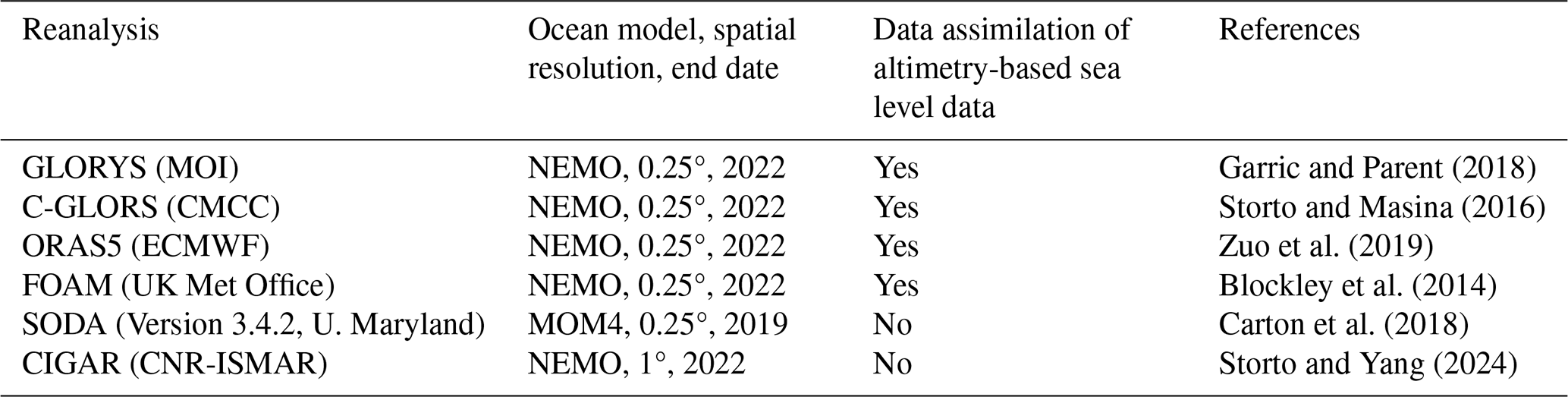
We consider six different ocean reanalyses with different characteristics as listed in Table 1. GLORYS, C-GLORS, ORAS5, and FOAM use the NEMO (Nucleus for European Modelling of the Ocean) ocean model and assimilate satellite altimetry-based sea level data. The SODA reanalysis is based on the MOM (Modular Ocean Model) developed by NOAA (National Oceanographic and Atmospheric Administration, USA) and does not include altimetry data. All reanalyses have a spatial resolution of 0.25°. In order to assess the regional sea level budget with another manometric component independent of satellite altimetry data, we also consider an ensemble reanalysis at lower resolution and without altimetry data assimilation (called CIGAR; see Table 1). This variety of reanalyses offers the opportunity to evaluate the degree of consistency of the manometric signal from reanalysis-based products.

Table 1 Characteristics of the six ocean reanalyses used in this study to estimate the manometric sea level change patterns independently from GRACE and GRACE-FO data.

To compare the manometric component derived from ocean reanalyses with the one based on GRACE and GRACE-FO, we added the contemporary GRD contribution to the reanalysis-based manometric sea level change. We used the sea level fingerprint data from Adhikari et al. (2019), which provide monthly contemporary GRD fingerprints at a 0.5° × 0.5° resolution. Because the Adhikari et al. (2019) data set ends in 2016, we linearly extrapolated the GRD fingerprints up to 2022 and added the corresponding trends to the ocean reanalyses-based manometric trends.

3.2 Method

Systematic corrections for both atmospheric loading and GIA effects are applied to altimetry-based and satellite gravimetry data sets, even though different models are used in each data set. The MOG2D (Carrere and Lyard, 2003) and inverse barometer model is used for altimetry data (http://www.aviso.altimetry.fr, last access: July 2024), while the GAD product is used for GRACE and GRACE-FO data (see Sect. 3.1.3). Likewise, the GIA corrections rely on the ICE6-G model for altimetry (Peltier et al., 2018), while GRACE data sets use either ICE6-G (Peltier et al., 2018) or the Caron et al. (2018) model.

All data sets were spatially interpolated onto a 1° × 1° grid and were averaged on a monthly basis. For spatial consistency, a common masking technique was applied to all gridded components. This mask covers latitudes from 66° S to 66° N, excludes inland seas, and omits coastal regions where the distance from land is less than 300 km.

All data sets span from January 2004 to December 2022, except for the oceanic reanalyses-based manometric components for which two study periods were considered, depending on the data set availability: January 2004–December 2019 and January 2004–December 2022.

Finally, seasonal signals (annual and semi-annual) were removed at each grid mesh of each data set through a simple least-squares adjustment of 6- and 12-month sinusoids, and a 3-month Lanczos filter was applied locally to each data set to remove high-frequency signals. The global mean trend of each data set computed over the study period was also removed before constructing the spatial trend maps.

For each gridded data set, we computed a trend uncertainty map.

For the altimetry data, we used the trend uncertainties provided by Prandi et al. (2021). These are based on a statistical computation which estimates via a generalized least-squares approach the total uncertainty in regional sea level trends due to all sources of errors affecting the altimetry-based sea level measurements (i.e. orbit, range, geophysical corrections, and intermission bias). In this approach, individual variance–covariance matrices describing time-correlated errors are computed for each source of uncertainty. Uncertainties from all sources are further combined by summing up the variances. Regional sea level trend uncertainties provided by Prandi et al. (2021) with this method applied to altimetry-based sea level grids of 2° × 2° resolution over 1993–2019 are on the order of 1 mm yr⁻¹ or less (1σ). The largest errors are located along the continental coastlines.

Since the SIO temperature and salinity data are not provided with uncertainties, we computed trend uncertainties for the thermosteric and halosteric components by considering the dispersion between two thermosteric/halosteric monthly data with respect to their mean: the SIO product used here and the EN4 T/S database, version 2.2 (https://www.metoffice.gov.uk/hadobs/en4/download-en4-2-2.html, last access: July 2024; Good et al., 2013). We estimated the thermosteric and halosteric trend uncertainty at each grid mesh from the dispersion between the two data sets (SIO and EN4) around the mean. For the total steric, thermosteric and halosteric trend uncertainties were quadratically combined.

As the ensemble mean of the 60 SH GRACE solutions is provided with trend uncertainties (adapted from Blazquez et al., 2018), these are used here for both GRACE-based manometric components (i.e. the ensemble mean mascon and the SH solutions).

Finally, for the uncertainties in the residual trend map (based on GRACE for the manometric component), we quadratically combined trend uncertainties in all components at each grid mesh.

Please note that the reanalyses used here do not provide uncertainty estimates.

In Fig. S1 of the Supplement are shown trend and associated trend uncertainty maps for the altimetry-based sea level, components, and residuals. Note that for altimetry-based sea level and components, the trend uncertainty map includes the global mean trend uncertainty (of smaller magnitude than the regional trends). Uncertainties correspond to 1σ errors.

4 Results: regional sea level trend budget with GRACE and Argo

4.1 Trend patterns in observed sea level, components, and residuals

Figure 1 shows the maps of altimetry-based sea level trends, of the GRACE- and Argo-based component trends, and of the residual trends (i.e. trend differences between altimetry-based sea level and sum of components). Hatched areas in the figures correspond to regions where the signal-to-noise ratio is not significant. This is based on comparing at each grid mesh the observed trend with the trend uncertainty (shown in Fig. S1). From Fig. 1, we note that except for the elongated negative pattern east of the Philippines in the western tropical Pacific, the altimetry-based sea level trends are significant everywhere. Concerning the GRACE-based manometric component, trends are not significant over a large portion of the northeastern Atlantic. The halosteric map displays a few regions where the trends are not significant. Most are located in the Southern Hemisphere. Accordingly, these translate into the total steric map. Finally, the residual trend map shows that the signal is significant essentially in areas where the residual trends are positive. Over several hatched areas, the residual trends are not significantly different from zero. This concerns most of the Pacific Ocean and a portion of the South Atlantic Ocean.

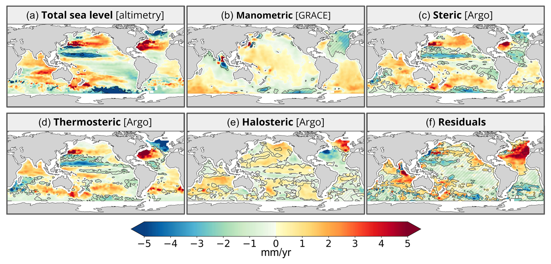
Figure 1 Sea level trends over January 2004 to December 2022 in total altimetry-based sea level (a), manometric component based on GRACE mascons (b), Argo-based total steric (c), thermosteric, and halosteric components, (d, e) and budget residual trends (observed sea level minus sum of components) (f). The hatched areas correspond to regions where the signal trend value is not significant compared to the corresponding trend uncertainties.

Visual inspection of Fig. 1 confirms earlier findings; i.e. the observed regional trend patterns are dominated by the thermosteric trend patterns (as expected; e.g. Stammer et al., 2013; Hamlington et al., 2020; Cazenave and Moreira, 2022). In the North Atlantic, thermosteric and halosteric trends have opposite signs. Except for two spots of high signal along the coasts of northern Indonesia and Japan due to the solid Earth response to the Sumatra and Tohoku earthquakes in 2004 and 2011 respectively (not removed here), the manometric trend map is dominated by large-scale patterns, positive over almost the whole Pacific, as well as over the South Atlantic Ocean and southwestern Indian Ocean. The absence of small-scale patterns likely results from the lower resolution of GRACE and Argo data compared to other data sets.

The residual trend map shows that in many regions, the sum of components cancels out the observed trends. This is the case over most of the Pacific Ocean and part of the South Atlantic Ocean, and southwestern Indian Ocean. In these regions, the residuals are not significantly different from zero, which suggests that the regional sea level budget can be considered as closed.

In the eastern Indian Ocean, along the coast of northern Indonesia, the positive residuals are related to the 2004 Sumatra earthquake The same is true for the positive residuals east of Japan and associated with the 2011 Tohoku earthquake. Besides these two regions, it is in the North Atlantic Ocean that the strongest positive residual trends are observed. In this region, altimetry-based and thermosteric sea level displays positive trends in the western part and negative trends south of Greenland, while opposite patterns are seen in the halosteric component. The strong residual signal in the North Atlantic is discussed in detail in Sect. 6.

4.2 GRACE data assessment

In this section, we explore the impact of the geocentre and GIA corrections applied to GRACE data on the residual trend map, considering that these two corrections remain imperfectly known (Blazquez et al., 2018). For that purpose, we decomposed the sea level budget components into spherical harmonics and computed the residuals for various configurations of low-degree harmonics (see Fig. S2 and Table S1 in the Supplement). Figure S2 and Table S1 show that degree 1,0 (related to the geocentre motion) and degree 2,1 (related to polar motion and GIA correction) harmonics contribute to the high positive residuals observed in the North Atlantic Ocean.

GRACE data are classically corrected for the geocentre motion when compared with altimetry data, in order to move GRACE observations from the centre of mass to the centre of figure of the reference system, in which the altimetry-based sea level is supposed to be also expressed after correcting the satellite orbits for the geocentre motion (Alexandre Couhert, personal communication, 2024).

Using the ensemble of 60 spherical harmonic solutions described in Sect. 3.1, we constructed an alternative ensemble of 60 solutions without applying the correction for the geocentre motion, i.e. keeping the GRACE observations in the centre of mass reference system. Comparing these two ensembles of solutions allows us to assess the influence of the geocentre correction on the manometric component and, consequently, on the residuals of the sea level budget. Figure 2 shows the impact of the geocentre correction on the manometric trends as well as on the associated residual trends. Not correcting for the geocentre motion reduces the residuals observed in the North Atlantic Ocean but increases the residual trends elsewhere, with larger residuals in almost all other ocean basins. Thus, even if the Sun et al. (2016) geocentre correction may not be optimal, it minimizes the residual trends, except in the northeastern Atlantic Ocean.

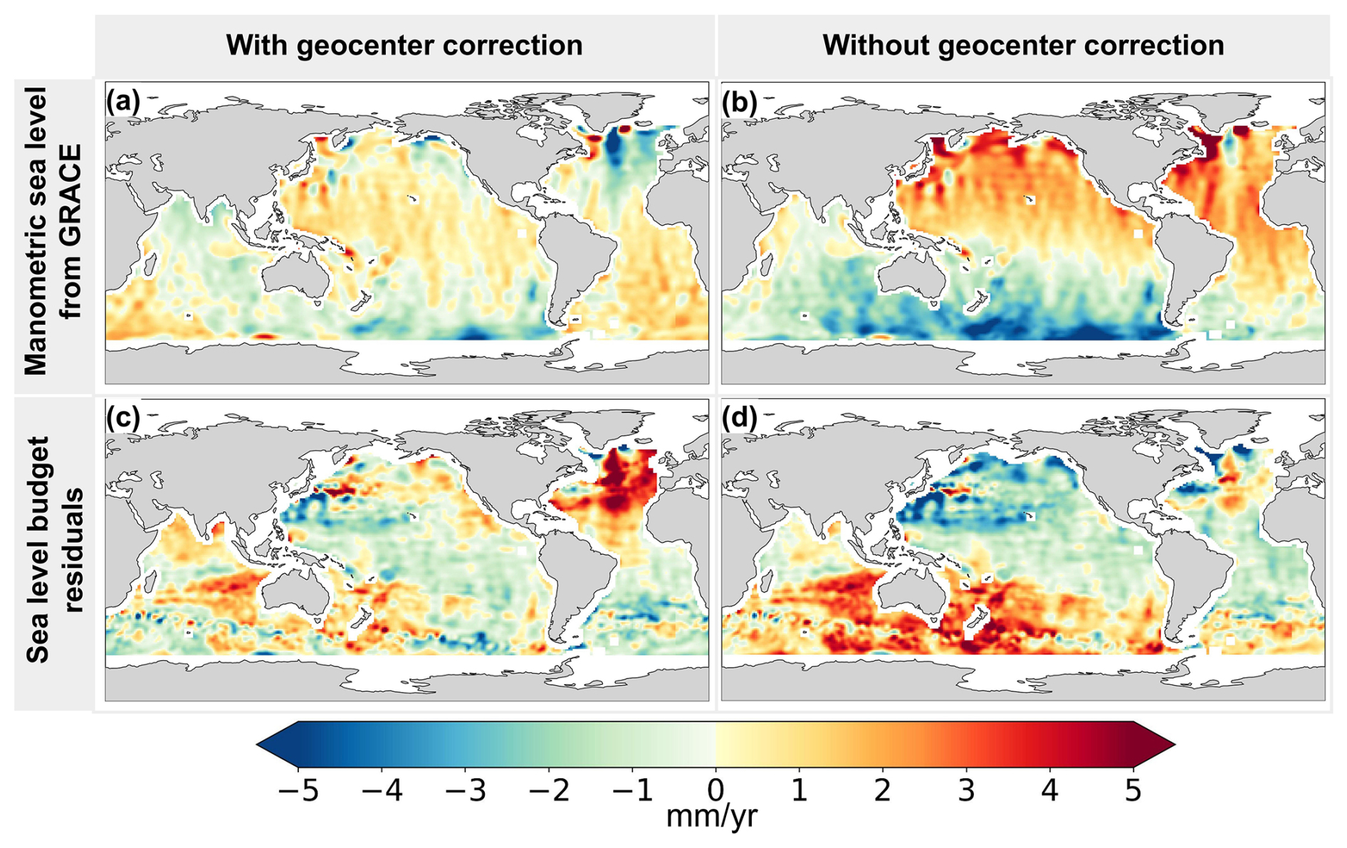
Figure 2 Sea level trends of the GRACE-based manometric component and corresponding budget residuals with and without the geocentre correction. (a) Manometric sea level trend map with the geocentre correction, (b) manometric sea level trend map without the geocentre correction, (c) sea level budget residual trend map computed with the manometric component corrected for the geocentre, and (d) sea level budget residual trend map computed with the manometric component not corrected for the geocentre.

If no geocentre correction is applied, the GRACE-based manometric component displays large-scale signals not observed by altimetry data so that the corresponding residual trends (Fig. 2d) also present unrealistic large-scale signals.

To estimate the impact of the GIA corrections on the manometric component and budget residuals, we further formed two separate subsets of 30 solutions each, for each GIA model (Peltier et al., 2018; Caron et al., 2018), applying the Sun et al. (2016) geocentre correction to each subset. Unlike for the geocentre case, no significant difference was observed.

5 Regional sea level trend budget using ocean reanalyses for the manometric component

As explained in Sect. 2, according to Gregory et al. (2019) and Camargo et al. (2023), the dynamic ocean mass redistribution due to ocean circulation changes can be estimated from the sterodynamic sea level corrected for local steric changes. Thus, in this study, we apply the Camargo et al. (2023) approach and use ocean reanalyses to estimate the manometric component, in order to further assess closure of the regional sea level budget.

As detailed above (Sect. 3), six different ocean reanalyses have been considered over their common period from January 2004 to December 2019. However, to compute the ensemble mean reanalysis, we discarded FOAM because of its spurious trends in the South Atlantic and the South Indian Ocean. Figure 3 shows the reanalysis-based manometric trend maps over 2004–2019, for each of the six data sets, as well as the ensemble mean based on CIGAR, C-GLORS, GLORYS, ORAS5, and SODA. The manometric components based on the two sets of GRACE solutions, restricted to this study period, are also shown.

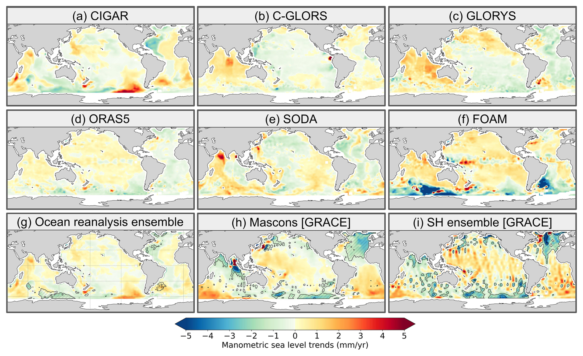
Figure 3 Reanalysis-based manometric trend maps over January 2004–December 2019 for each of the six ocean reanalyses: CIGAR, C-GLORS, GLORYS, ORAS5, SODA, and FOAM (a–f). Panel (g) shows the ensemble mean of the five reanalyses (CIGAR, C-GLORS, GLORYS, ORAS5, and SODA). Panels (h) and (i) refer to the manometric component from the GRACE mascon and GRACE spherical harmonic (SH) ensembles. Hatched areas in (g), (h), and (i) represent regions where the signal is not significant.

No uncertainties are provided with the reanalyses data so that it is not possible to highlight the areas where the signal is significant for the individual cases (Fig. 3a–d). This can be done however for the ensemble mean (Fig. 3g) where the errors are estimated from the dispersion of the five reanalyses (CIGAR, C-GLORS, GLORYS, ORAS5, and SODA) about the mean.

The six reanalyses provide quite different manometric trend patterns. The FOAM and ORAS5 patterns are quite similar in the Pacific and Indian oceans. In these regions, C-GLORS, CIGAR, and GLORYS show rough agreement. SODA's patterns differ from the other reanalyses everywhere, although they look similar to CIGAR in the Indian Ocean. As mentioned above, the FOAM-based manometric map shows spurious high trends in the South Atlantic and the South Indian Ocean. This is why it is not included in the ensemble mean.

Comparing ensemble mean reanalyses-based manometric maps with the GRACE-based manometric maps, we note the following: (1) the spatial patterns of the reanalysis-based manometric trend map have generally slightly lower amplitude than the GRACE ones in many regions, except around Antarctica, and (2) the manometric spatial trends of the ensemble mean reanalyses and GRACE have opposite signs in many regions, including in the North Atlantic.

The regional trend budget has been computed with each of the six reanalyses as well as for the ensemble mean (FOAM excluded), all other data being kept unchanged. The corresponding residual trend patterns are shown in Fig. 4.

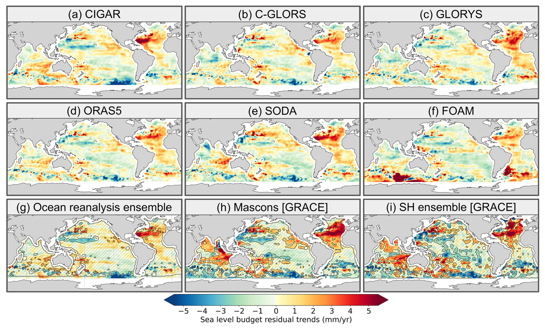
Figure 4 Residual trends of the regional sea level budget computed with each of the six reanalyses-based manometric components, as well as with the ensemble mean (FOAM excluded) (a–g) (with altimetry-based and steric components unchanged). GRACE-based residual trends for both mascon and spherical harmonic solutions are also shown (h–i). The period of analysis here is from January 2004 to December 2019. Hatched areas in (g), (h), and (i) represent regions where the signal is not significant.

Table 2 RMS of gridded residuals trends over 2004–2019, averaged over the Pacific, Indian, and North and South Atlantic oceans for the six reanalyses and GRACE mascon cases.

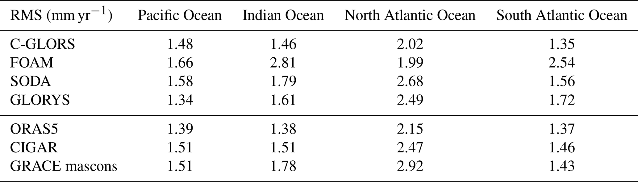
The CIGAR, C-GLORS, SODA, ORAS5, and GLORYS reanalyses give very similar residual trend patterns, even though SODA uses completely different ocean model and data assimilation schemes, and no altimetry-based sea level data are assimilated. Note that CIGAR also does not assimilate altimetry-based sea level anomaly data, but it is forced by the latest atmospheric reanalysis from ECMWF (unlike the other reanalyses) and embeds a daily varying runoff data set for freshwater discharge into the oceans. Again, one outlier is FOAM, which shows strong positive residual trends in the South Atlantic and South Indian Ocean. The ensemble mean residual trend map (FOAM excluded) displays slightly lower signal than the GRACE cases (compare panel g with panels h and i in Fig. 4). What is striking is that the two approaches (reanalyses and GRACE) show positive residual trends in the North Atlantic. However, the residuals are significantly stronger using GRACE, especially in the northeastern part of the Atlantic Ocean. This will be discussed in Sect. 6.

Table 2 shows the root mean square (RMS) of the gridded residual trends over 2004–2019, averaged over the Pacific, Indian, and North and South Atlantic oceans for the reanalyses and GRACE cases.

If we exclude FOAM, which displays higher RMS in the Indian and South Atlantic oceans than other reanalyses, Table 2 clearly shows systematically higher RMS (in the range 2–3 mm yr⁻¹) in the North Atlantic Ocean for the C-GLORS, SODA, GLORYS, and ORAS5 reanalyses as well as for GRACE mascons.

Because four of the reanalyses used above assimilate altimetry data (i.e. C-GLORS, GLORYS, ORAS5, and FOAM), our approach may introduce some circularity to the regional sea level budget assessment. This is the reason for also using reanalyses without altimetry data assimilation (SODA and CIGAR). Here we focus on CIGAR and extend the study period to December 2022. Comparing the manometric components of two reanalyses with and without altimetry data assimilation (e.g. C-GLORS and CIGAR, noting however that they differ in terms of resolution, configuration, and forcing; Fig. 4) shows some differences locally, in particular in the northwestern Atlantic and North Indian oceans. However, the residual trend maps are very similar. Figure 5 shows manometric and residual trend maps based on CIGAR, GRACE mascons, and GRACE SH ensemble, extended until 2022. Overall, the patterns are qualitatively similar to those of the shorter period 2004–2019 (Figs. 3 and 4). Thus, adding three more years does not change the previous conclusion, i.e. that significant residual trends are observed in the North Atlantic (and around Antarctica as well). But the residual patterns in the North Atlantic are noticeably different between CIGAR and GRACE, the maximum signal being located in the western part of the basin for CIGAR and in the eastern part for GRACE.

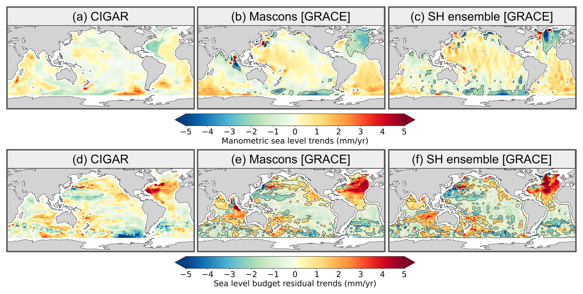
Figure 5 Manometric component based on the CIGAR reanalysis (reanalysis without altimetry data assimilation) (a) and the two GRACE solutions (b, c). Sea level budget residuals using the CIGAR-based manometric component (d) and the two GRACE manometric components (e, f). The period of analysis here is from January 2004 to December 2022. Hatched areas in (b), (c), (e), and (f) represent regions where the signal is not significant.

One may wonder whether the salinity drift observed in some Argo floats as of 2015 has impacted the CIGAR reanalysis since, unlike for altimetry data, $T/S$ data are assimilated during the reanalysis integration, thus non-linearly interacting with dynamical processes. In the reanalysis, the treatment of the salinity drift simply consisted in rejecting data that Argo had flagged for rejection in the delayed mode. But this may not fully guarantee that all bad salinity data have been discarded, possibly leading to a shift in the circulation. However, to compute the reanalysis-based manometric component, the local steric contribution has been removed. Thus, any effect of the spurious Argo salinity drift may be considered as minimal.

6 Residual trends in the North Atlantic Ocean

In this section, we focus on the North Atlantic Ocean where significant positive residuals are observed when using either GRACE or the CIGAR reanalysis for estimating the manometric component.

Figure 6 shows each component of the budget over the North Atlantic Ocean over January 2004–December 2022, including the three manometric component estimates: GRACE mascons, ensemble mean GRACE SH, and CIGAR reanalysis. Associated residual maps (all components unchanged except the manometric one) are also shown.

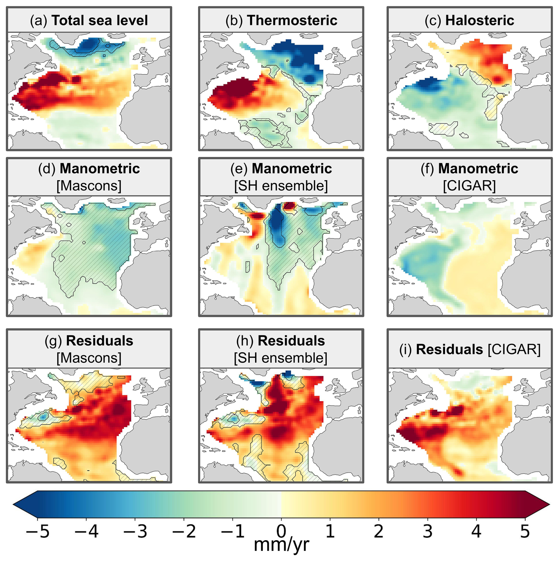
Figure 6 North Atlantic Ocean sea level trends (mm yr⁻¹) over January 2004 to December 2022: observed altimetry-based sea level (a), Argo-based thermosteric and halosteric components (b, c), manometric components from GRACE mascons (d), ensemble mean GRACE spherical harmonics (e), and derived from CIGAR reanalysis (f). Sea level budget residuals (observed sea level trends minus sum of component trends) using GRACE mascons (g), ensemble mean GRACE spherical harmonics (h), and CIGAR (i). Hatched areas represent regions where the signal is not significant.

The North Atlantic Ocean residuals of all three manometric component cases (GRACE mascons, ensemble mean GRACE spherical harmonics, and CIGAR) show a positive signal. However, the patterns are significantly different between the reanalysis and GRACE cases. They are localized in the western part of the tropical North Atlantic Ocean with the CIGAR reanalysis and in the eastern part (between the Strait of Gibraltar and the Bay of Biscay) with GRACE mascons. The residuals based on the ensemble mean GRACE spherical harmonics display a strong north–south signal in the mid North Atlantic, likely due to north–south stripe noise affecting spherical harmonic solutions (Blazquez et al., 2018).

To further investigate the North Atlantic sea level misclosure, we computed the North Atlantic sea level budget after geographically averaging each component over the region, using GRACE mascons for the manometric component. This is shown in Fig. 7, along with the sea level budget, averaging the data globally but excluding the North Atlantic Ocean.

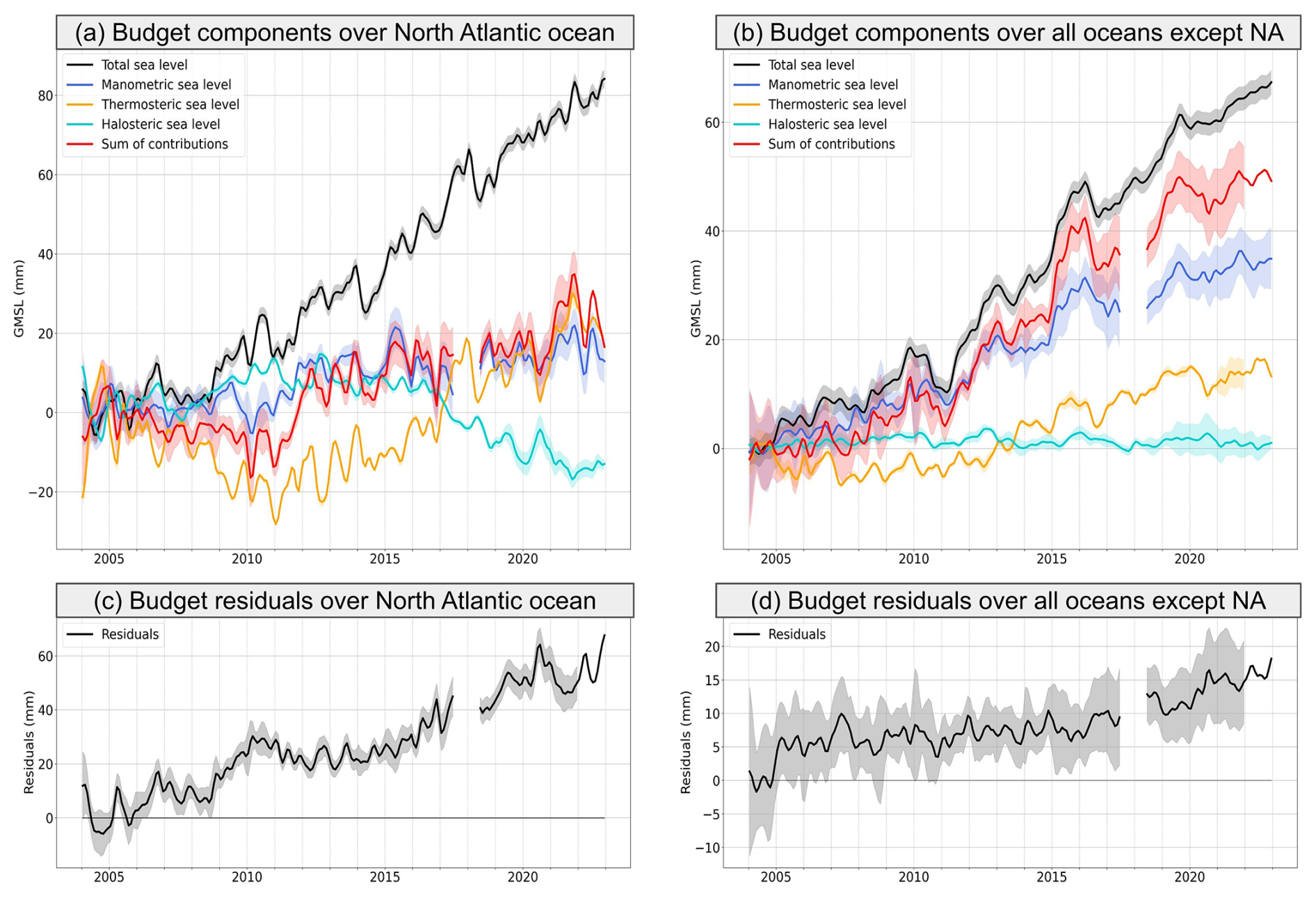
Figure 7 Regionally averaged sea level budget for January 2004 to December 2022, over the North Atlantic Ocean (a) and over all oceans except the North Atlantic (NA) (b). In each panel the altimetry-based sea level (black curve), the thermosteric and halosteric components (orange and turquoise curves), the manometric component (GRACE mascons, blue curve), and the sum of all components (red curve) are shown. The panels (c) and (d) show the corresponding residuals (observed sea level minus sum of components). Shaded areas represent the standard 1σ uncertainties.

Figure 7 well confirms the non-closure of the trend budget over the North Atlantic Ocean. While in Fig. 7c the North Atlantic residuals display a positive trend over the whole period (like in Fig. 7d), there is a clear shift towards higher residuals around 2015 that may be directly linked to the strongly negative trend as of 2015 of the halosteric component of the North Atlantic (Fig. 7a). A similar finding is provided in Mu et al. (2024).

In order to check whether the North Atlantic residual signal better fits a trend over the study period rather than a low-frequency oscillation, we performed an EOF (empirical orthogonal function) decomposition over 2004–2022 of the gridded residual time series (considering the GRACE SH solution for the manometric component) (see Fig. S3 in the Supplement, showing the first two EOF modes). Mode 1 is dominated by a strong residual trend in the North Atlantic. Its spatial map is very similar to the residual map. Mode 2 shows an oscillation of period ∼ 11 years, on which shorter fluctuations related to ENSO are superimposed. This EOF decomposition of the residuals confirms the dominant trend contribution of the North Atlantic over the study period.

7 Conclusion

In this study, we have revisited the regional sea level trend budget over the GRACE and Argo era. Using different data sets for the manometric component (GRACE and ocean reanalyses), we found significant non-closure of the trend budget in the North Atlantic Ocean in all studied cases. However, the residual patterns are not localized over the same areas in the GRACE and ocean reanalyses cases. They are stronger in the northeastern Atlantic Ocean when considering the GRACE manometric component (mascon solution), while they are more localized in the northwestern tropical part with the reanalysis-based manometric component. The sea level budget averaged over the whole North Atlantic Ocean leads us to suspect the steric contribution, especially the halosteric component as the main contributor to the budget non-closure in this region, considering that the global budget without the North Atlantic region is closed within the error bars. Although we chose the SIO data set to estimate the steric component, considering that the salinity data had been corrected for the Argo float instrumental drift that led to spurious salinity measurements, our study points to remaining errors affecting the halosteric component, especially as of 2015. Mu et al. (2024) also report a potential salinity bias in the Argo data set of the North Atlantic. Our results suggest that the salinity adjustment to the WOCE salinity climatology proposed by the SIO methodology may not fully correct for the rapid salinity drift experienced by some Argo floats. However, the different locations of the North Atlantic residual patterns when considering the reanalyses or GRACE for the manometric component, as well as larger residuals in the northeastern Atlantic Ocean in the GRACE case, suggest that uncertainty in GRACE data also plays a role. In other oceanic regions, a few areas display small-scale residual structures (e.g. in the North Pacific, eastern Pacific, and northwestern Indian Ocean). This may eventually result from differences in resolution of the gridded data sets used in this study (e.g. satellite altimetry better resolves small-scale features than GRACE or Argo), even though the same low-pass filter was applied to all data sets.

The problem of the North Atlantic halosteric component highlighted in our regional trend budget study needs to be fixed up at the processing level of the Argo-based measurements. Our findings are helpful to the scientific groups involved in the Argo network as we can identify regions where the salinity contribution to regional sea level change appears to be spurious. This may help them in refining their investigations on the quality control checks to be applied to the Argo profiles. In addition, detailed investigation of the GRACE contribution to the residuals of this region should also be carried out in parallel. Our study highlights the necessity of applying consistent data processing and using similar reference systems for satellite altimetry and gravimetry data. Improved data should indeed be made available to the community, not only for sea level budget assessments but also for other applications in oceanography or climate-related research (i.e. for Earth's energy imbalance studies based on sea level budget approaches).