the Creative Commons Attribution 4.0 License.
the Creative Commons Attribution 4.0 License.
 | 11 Jun 2024
Anthropogenic CO2, air–sea CO2 fluxes, and acidification in the Southern Ocean: results from a time-series analysis at station OISO-KERFIX (51° S–68° E)
Nicolas Metzl
Claire Lo Monaco
Coraline Leseurre
Céline Ridame
Gilles Reverdin
Thi Tuyet Trang Chau
Frédéric Chevallier
Marion Gehlen
The temporal variation of the carbonate system, air–sea CO2 fluxes, and pH is analyzed in the southern Indian Ocean, south of the polar front, based on in situ data obtained from 1985 to 2021 at a fixed station (50°40′ S–68°25′ E) and results from a neural network model that reconstructs the fugacity of CO2 (fCO2) and fluxes at monthly scale. Anthropogenic CO2 (Cant) is estimated in the water column and is detected down to the bottom (1600 m) in 1985, resulting in an aragonite saturation horizon at 600 m that migrated up to 400 m in 2021 due to the accumulation of Cant. At the subsurface, the trend of Cant is estimated at µmol kg−1 yr−1 with a detectable increase in the trend in recent years. At the surface during austral winter the oceanic fCO2 increased at a rate close to or slightly lower than in the atmosphere. To the contrary, in summer, we observed contrasting fCO2 and dissolved inorganic carbon (CT) trends depending on the decade and emphasizing the role of biological drivers on air–sea CO2 fluxes and pH inter-annual variability. The regional air–sea CO2 fluxes evolved from an annual source to the atmosphere of 0.8 molC m−2 yr−1 in 1985 to a sink of −0.5 molC m−2 yr−1 in 2020. Over 1985–2020, the annual pH trend in surface waters of per decade was mainly controlled by the accumulation of anthropogenic CO2, but the summer pH trends were modulated by natural processes that reduced the acidification rate in the last decade. Using historical data from November 1962, we estimated the long-term trend for fCO2, CT, and pH, confirming that the progressive acidification was driven by the atmospheric CO2 increase. In 59 years this led to a diminution of 11 % for both aragonite and calcite saturation state. As atmospheric CO2 is expected to increase in the future, the pH and carbonate saturation state will decrease at a faster rate than observed in recent years. A projection of future CT concentrations for a high emission scenario (SSP5-8.5) indicates that the surface pH in 2100 would decrease to 7.32 in winter. This is up to −0.86 lower than pre-industrial pH and −0.71 lower than pH observed in 2020. The aragonite undersaturation in surface waters would be reached as soon as 2050 (scenario SSP5-8.5) and 20 years later for a stabilization scenario (SSP2-4.5) with potential impacts on phytoplankton species and higher trophic levels in the rich ecosystems of the Kerguelen Islands area.
- Article
(12074 KB) - Full-text XML
-
Supplement
(2828 KB) - BibTeX
- EndNote


The ocean plays an important role in mitigating climate change by taking up a large part of the excess of heat (Cheng et al., 2020a; Fox-Kemper et al., 2021) and of CO2 released by human activities (Sabine et al., 2004; Gruber et al., 2019a; Canadell et al., 2021). Since 1750, the global ocean has captured 185±35 PgC (petagram of carbon) from a total of 700±75 PgC of anthropogenic carbon emissions from fossils fuels and land-use changes (Friedlingstein et al., 2022). The oceanic sink for anthropogenic CO2 increased progressively from 1.1±0.4 PgC yr−1 in the 1960s to 2.3±0.4 PgC yr−1 in the 2000s. Over the decade 2012–2021, the partitioning of the anthropogenic CO2 uptake was roughly equal between the ocean (2.9±0.4 PgC yr−1) and the land (3.1±0.6 PgC yr−1) (Friedlingstein et al., 2022). This partitioning has been confirmed for the decade 2013–2022 (Friedlingstein et al., 2023).
Ocean observations indicate that the Southern Ocean (SO) south of 45° S has been accumulating each year about 0.5 PgC yr−1 since the 1990s (e.g., Takahashi et al., 2009a, b; Lenton et al., 2013; Rödenbeck et al., 2013; Long et al., 2021; Fay et al., 2024; Gray, 2024). Results based on BGC-Argo floats (Southern Ocean Carbon and Climate Observations and Modeling project, SOCCOM) suggest that the CO2 sink in the SO might be much lower (0.16 PgC yr−1 south of 44° S for the period 2015–2017; Gray et al., 2018; Bushinsky et al., 2019), but there is an ongoing debate on the size of the carbon sink in this region depending the periods and methods (Long et al., 2021; Sutton et al., 2021; Hauck et al., 2023b; Gray, 2024). It is also well established that the CO2 sink in the SO undergoes substantial decadal variability first documented for the 1990s (Le Quéré et al., 2007; Metzl, 2009; Lenton et al., 2013) and subsequently identified for the period 1982–2018 (Landschützer et al., 2015; Keppler and Landschützer, 2019; Mackay et al., 2022; Hauck et al., 2023a, b). However as for the mean state, there are also uncertainties on both the magnitude and phasing of decadal variability in the SO carbon sink mainly due to insufficient sampling (Gloege et al., 2021; Hauck et al., 2023a, b). A recent extension of the period to 1957–2020 suggests that the inter-annual to decadal variability of the SO CO2 sink was most pronounced after the 1980s (Rödenbeck et al., 2022; Bennington et al., 2022). Whatever the variability of the SO CO2 sink since the 1960s, the ocean continuously absorbs atmospheric CO2 ,and the distribution of anthropogenic CO2 (Cant) in the SO is now relatively well documented (e.g., Pardo et al., 2014; Gruber et al., 2019a) thanks to the Global Ocean Data Analysis Project (GLODAP) data synthesis effort for the global ocean (Olsen et al., 2016, 2019, 2020). The SO takes up about 40 % of the total anthropogenic carbon that enters the ocean (Khatiwala et al., 2013; Gruber et al., 2019a).
The anthropogenic CO2 uptake in the ocean results in lowering carbonate ion concentrations and pH, a chemical process termed “ocean acidification” (OA) (Caldeira and Wickett 2003; Doney et al., 2009). This decreases the saturation state with respect to carbonate minerals (aragonite, ΩAr, and calcite, ΩCa), a process most pronounced in the cold waters at high latitudes where the saturation state is naturally low (Orr et al., 2005; Takahashi et al., 2014; Jiang et al., 2015). The first estimate of Cant distribution in the global ocean (for a nominal year 1994; Sabine et al., 2004) shows that the accumulation of Cant led to an upward migration of the ΩAr and ΩCa saturation horizon in all ocean basins (Feely et al., 2004). This change is particularly pronounced south of the polar front (PF) in the SO due to both Cant uptake and the enhanced upwelling of carbon-rich deep waters (e.g., Hauck et al., 2010; Pardo et al., 2017). It has been suggested, through numerical studies, that depending on future CO2 emission levels, surface waters in the SO could reach undersaturation state for aragonite by 2030–2050 (Orr et al., 2005; Gangstø et al., 2008; McNeil and Matear, 2008; Negrete-Garcia et al., 2019). Such a change would have multiple and detrimental impacts on marine ecosystems (Fabry et al., 2008; Doney et al., 2012; Bopp et al., 2013), in particular calcifying marine organisms, especially aragonite producers such as pteropods (Hunt et al., 2008; Gardner et al., 2023), as well as calcite-producing planktonic foraminifera (Moy et al., 2009), coccolithophorids (Beaufort et al., 2011), and non-calcifying species such as the abundant SO diatoms (e.g., Benoiston et al., 2017; Petrou et al., 2019; Weir et al., 2020; Duncan et al., 2022) and krill (Kawaguchi et al., 2013).
Hindcast simulations with global ocean biogeochemical models (GOBMs), as well as projections with Earth system models (ESMs), have been used to evaluate the ocean carbon cycle over the past decades and future changes in Cant storage, ocean acidification, or impacts of global changes on marine ecosystems. However, current model-based estimates of the contemporary SO CO2 sink are subject to relatively large uncertainties (e.g., Long et al., 2013; Gooya et al., 2023; Hauck et al., 2020, 2023a, b; Mayot et al., 2023; DeVries et al., 2023). Differences between GOBMs can reach up to 0.7 PgC yr−1 in the SO (Hauck et al., 2020), which is roughly equivalent to the mean climatological flux of 0.5 PgC yr−1 (McNeil et al., 2007; Takahashi et al., 2009a, b; Lenton et al., 2013). At the high latitudes of the SO (>50° S) for the 2010s, ESMs from the Coupled Model Intercomparison Project Phase 6 (CMIP6) simulated either a large sink or a modest source of CO2 (McKinley et al., 2023). This is mainly due to incorrect or missing physical and/or biological processes in the models (e.g., Pilcher et al., 2015; Kessler and Tjiputra, 2016; Mongwe et al., 2018; Lerner et al., 2021), leading to biases in the seasonality of temperature, dissolved inorganic carbon CT, partial pressure of CO2 (pCO2), air–sea CO2 fluxes, pH, or Ω (e.g., McNeil and Sasse, 2016; Rodgers et al., 2023; Rustogi et al., 2023; Joos et al., 2023). Such model imperfections should be resolved to gain reliability in future projections of CO2 uptake, OA, productivity, and the responses of the marine ecosystems (Frölicher et al., 2015; Hauck et al., 2015; Sasse et al., 2015; Kessler and Tjiputra, 2016; McNeil and Sasse 2016; Kwiatkowski and Orr, 2018; Negrete-Garcia et al., 2019; Burger et al., 2020; Krumhardt et al., 2022; Jiang et al., 2023; Mongwe et al., 2024). In this context, long-term biogeochemical observations are particularly valuable to quantify and understand recent past and current changes, and ultimately evaluate model simulations, as often concluded in modeling studies (e.g., Kessler and Tjiputra, 2016; Gooya et al., 2023; Wright et al., 2023; Hauck et al., 2023a; Mayot et al., 2023; Rodgers et al., 2023).
Table 1Trends of oceanic fCO2 (µatm yr−1) and pH (per decade) in the Southern Ocean south of the polar front based on observations. IO: Indian Ocean sector. PO: Pacific Ocean sector. AO: Atlantic Ocean sector. SO SPSS: Southern Ocean subpolar seasonally stratified biome (around 50–60° S). PZ: polar zone. NR: not reported. Standard deviations when available are given in brackets.
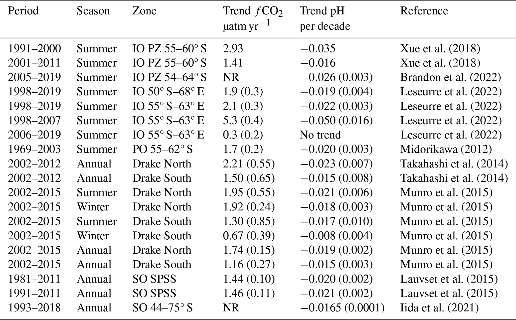
Although the SO south of the polar front remains much less observed than other oceanic regions, several observations-based studies have estimated the decrease in pH in surface waters in response to the increase in oceanic CO2 fugacity, fCO2 (Midorikawa et al., 2012; Takahashi et al., 2014; Lauvset et al., 2015; Munro et al., 2015; Xue et al., 2018; Iida et al., 2021; Leseurre et al., 2022; Brandon et al., 2022). Results showed a large range in the pH trends from −0.008 −0.035 per decade depending on the period and the region of interest. Most of these analyses were based on summer observations (Table 1), and some studies highlighted contrasting pH trends on a 5–10-year timescale probably linked to large-scale climate variability such as the Southern Annular Mode (SAM) (e.g., Xue et al., 2018). Given such variability, it is important to continue monitoring fCO2 and pH trends and, if possible, at different seasons as future change in CO2 uptake and potential tipping points of the carbonate saturation state also depend on seasonality (Sasse et al., 2015). The above observational studies were dedicated to pH changes in surface waters. In contrast to northern high latitudes (e.g., Olafsson et al., 2009, 2010; Franco et al., 2021; Skjelvan et al., 2022), few studies in the SO evaluated decadal changes of carbonate system properties and acidification in the water column based on time-series stations.These changes in the SO water column were investigated from data collected during cruises generally 3 to 15 years apart (e.g., Hauck et al., 2010; Van Heuven et al., 2011; Pardo et al., 2017; Tanhua et al., 2017; Carter et al., 2019).
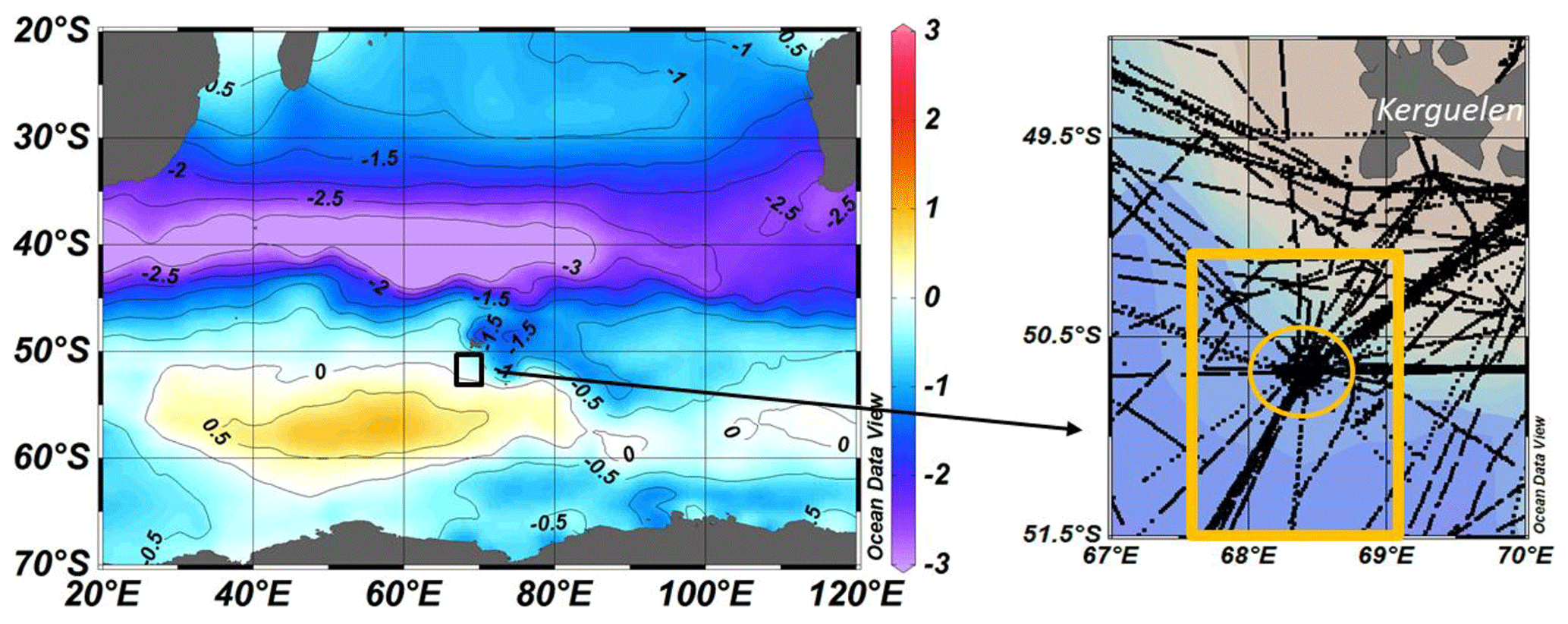
Figure 1Left: annual air–sea CO2 flux (molC m−2 yr−1) in the southern Indian Ocean for year 2020 from the FFNN model (negative flux for ocean sink, positive flux for ocean source). The black box identifies the location of the study southwest of Kerguelen Islands. Right: track of cruises with underway fCO2 data southwest of Kerguelen Islands. The station at 50°40′ S–68°25′ E occupied in 1985, 1992–1993, and 1998–2021 is indicated by a yellow circle. The yellow square is the region selected to calculate the mean values from the underway surface observations and from the FFNN model. Figures produced with Ocean Data View (ODV; Schlitzer, 2018).
The present study complements in time, seasons, and in the water column the surface fCO2 and pH trends investigated by Leseurre et al. (2022) in different regions of the southern Indian Ocean for the period 1998–2019 during austral summer. South of the PF around 50° S, Leseurre et al. (2022) showed that in summer the surface fCO2 increase and pH decrease over 20 years were mainly driven by the accumulation of anthropogenic CO2 by about µmol kg−1 yr−1 and by a small warming of °C yr−1. In addition Leseurre et al. (2022) showed that in the recent decade, 2007–2019, the fCO2 trend was low ( µatm yr−1) compared to the previous decade ( µatm yr−1 over 1998–2007), highlighting the sensitivity of the fCO2 and pH trends to the selected time period (especially during summer). In particular, they observed relatively stable pH values over 2010–2019 (i.e., no decrease in pH) with no clear explanation on the origin of the slow-down of the fCO2 and pH trends in surface waters south of the PF in recent years. To complement the analysis by Leseurre et al. (2022) based on summer observations over the period 1998–2019, this study focuses on one location regularly visited south of the polar front (around 50° S–68° E southwest of Kerguelen Island; Fig. 1). The analysis period is first extended back to 1985 and forward to 2021 to investigate the recent status of fCO2 and pH. We also evaluate the trends during late winter using sparse data in October/November. The combination of in situ observations and monthly estimates from a neural network model over the period 1985–2020 (Chau et al., 2022) enables us to assess potential changes in seasonality of the surface ocean carbonate system (including fCO2, CT, pH, Ω) as suggested in recent decades or in future scenarios (Hauck and Völker, 2015; Gallego et al., 2018; Landschützer et al., 2018; Kwiatkowski and Orr, 2018; Kwiatkowski et al., 2020; Lerner et al., 2021; Fassbender et al., 2022; Yun et al., 2022; Rodgers et al., 2023; Joos et al., 2023). The changes observed in surface waters will be related to changes in Cant concentrations estimated in the water column and will be complemented by an analysis of OA at depth between 1985 and 2021. Finally we will explore the long-term change of surface fCO2 and pH since the 1960s and potential future changes of the carbonate system at this time-series site.
2.1 Study area and data selection
This study focuses on a high-nutrient low-chlorophyll area (HNLC; Minas and Minas, 1992) in the Indian sector of the Southern Ocean (SO) in the Permanent Open-Ocean Zone (POOZ) south of the polar front (PF) and southwest of Kerguelen Islands (around 50° S–68° E, Fig. 1). The Kerguelen Plateau is an extended topographic feature that controls part of the Antarctic Circumpolar Current (ACC) and generates eddies (Daniault and Ménard, 1985) and the northward deflection of the PF just east of the island (Pauthenet et al., 2018). The plateau is also a region of relatively high chlorophyll-a (Chl-a) concentration (Moore and Abbott, 2000; Mongin et al., 2008) and strong CO2 uptake during austral spring–summer that contrasts with the weaker sink over the POOZ/HNLC (Metzl et al., 2006; Jouandet et al., 2008, 2011; Lo Monaco et al., 2014; Leseurre et al., 2022). The POOZ/HNLC region west (upstream) of the Kerguelen Plateau is characterized by rather stable water mass properties (temperature, salinity, oxygen, or nutrients) over time and low eddy activity compared to the plateau (Daniault and Ménard, 1985; Chapman et al., 2015; Dove et al., 2022). In this region, located in the deep Enderby Basin, the flow is not constrained by topography and there is no local upwelling that would import CT-rich waters to the surface layers as observed on the eastern side of the Kerguelen Plateau (Brady et al., 2021).
The Indian sector of the SO is also recognized to host the strongest winds in the SO leading to year-round high gas transfer coefficients (Wanninkhof and Trinanes, 2017). As a result, and in contrast to the Atlantic sector of the SO, the Indian region south of 45° S was a periodic annual CO2 source, especially in the 1960s to the 1980s (Rödenbeck et al., 2022; Bennington et al., 2022; Prend et al., 2022; Gray, 2024). In the POOZ–HNLC region, high winter wind speed (monthly average up to 16 m s−1) and associated heat loss drive deep mixing. Deep winter mixing entrains subsurface properties to the surface layer and increases surface CT concentrations, leading to wintertime outgassing of CO2 (Metzl et al., 2006). This combination of characteristics makes the region an ideal test bed for 1-D modeling studies investigating the temporal dynamics and drivers of biogeochemical processes including nutrients, iron, phytoplankton, and carbon (Pondaven et al., 1998, 2000; Louanchi et al., 1999, 2001; Jabaud-Jan et al., 2004; Metzl et al., 2006; Mongin et al., 2006, 2007; Kane et al., 2011; Pasquer et al., 2015; Demuynck et al., 2020).
Here we used surface and water column observations around location 50° 40′ S–68° 25′ E (Fig. 1, Table S1 in the Supplement), historically called KERFIX station (KERguelen FIXed station) sampled from 1990 to 1995 in the framework of the WOCE and JGOFS programs (Jeandel et al., 1998). The station was first occupied in March 1985 during the INDIGO-1 cruise (Indian Ocean Geochemistry; Poisson, 1985; Poisson et al., 1988), and since 1998 it has been regularly visited during the OISO cruises (Océan Indien Service d'Observations; Metzl and Lo Monaco, 1998, https://doi.org/10.18142/228). The regular occupation from 1985 to 2021 makes it the longest time-series station in the Southern Ocean POOZ/HNLC area for investigating the inter-annual to decadal trends of carbonate properties in surface waters and across the water column (0–1600 m). Despite the occasional large anomalies in surface waters properties (e.g., lower temperature in December 1998, lower salinity in February 2013), we consider all observations selected for this study both in surface waters and the water column to be representative of the water masses in this POOZ/HNLC region upstream of the Kerguelen Plateau.
Data for the period 1985–2011 were extracted from the GLODAP data product, version V2.2021 (Lauvset et al., 2021a, b; Table S1a). Observations collected during OISO cruises from 2012 to 2021 will be included in GLODAP-V3. For the surface water properties, all available underway fCO2 data were selected (Fig. 1). This includes one cruise in November 1962 (Keeling and Waterman, 1968) and 41 cruises from 1991 to 2021 (Table S1b). All surface temperature, salinity, and fCO2 data were extracted from the SOCAT (Surface Ocean CO2 Atlas) data-product version v2022 (Bakker et al., 2016, 2022) and have an accuracy of fCO2 between 2 and 5 µatm.
2.2 Methods
The methods for surface underway fCO2 and biogeochemical properties (oxygen, CT, total alkalinity AT, nutrients) in the water column for the INDIGO-1, KERFIX, and OISO cruises were described in previous studies (e.g., Poisson et al., 1993; Louanchi et al., 2001; Metzl et al., 2006; Metzl, 2009; Mahieu et al., 2020; Leseurre et al., 2022). Here we briefly recall the methods for underway fCO2 and water column observations.
2.2.1 Surface fCO2 data
For fCO2 measurements in 1991–2021, sea-surface water was continuously equilibrated with a “thin film” type equilibrator thermostated with surface seawater (Poisson et al., 1993). The xCO2 in the dried gas was measured with a non-dispersive infrared analyzer (NDIR, Siemens ULTRAMAT 5F or 6F). Standard gases for calibration (around 270, 350, and 490 ppm) were measured every 6 h. To correct xCO2 dry measurements to fCO2 in situ data, we used polynomials from Weiss and Price (1980) for vapor pressure and from Copin-Montégut (1988, 1989) for temperature. Note that when incorporated in the SOCAT database, the original fCO2 data are recomputed (Pfeil et al., 2013) using temperature correction from Takahashi et al. (1993). Given the small difference between equilibrium temperature and sea surface temperature ( °C on average for the cruises in 1998–2021), the fCO2 data from SOCAT used in this analysis (Bakker et al., 2022) are almost identical (within 1 µatm) to the original fCO2 values from our cruises (http://www.ncei.noaa.gov/access/ocean-carbon-data-system/oceans/VOS_Program/OISO.html, last access: 15 January 2024).
2.2.2 Water column data
Over the period 1990–1995, water samples were collected during the KERFIX program on the ship La Curieuse at standard depths using 8 L Niskin bottles mounted on a stainless-steel cable and equipped with reversing SIS pressure and temperature probes. Methods and accuracy for the geochemical measurements used in this analysis (AT, CT, oxygen, nutrients) are detailed by Jeandel et al. (1998) and by Louanchi et al. (2001). From 1998 onwards, the station was occupied within the framework of the OISO long-term monitoring program on board the R/V Marion Dufresne. We used conductivity–temperature–depth (CTD) sensors mounted on 24 rosette samplers equipped with 12 L Niskin bottles. Temperature and salinity measurements have an accuracy of 0.002 °C and 0.005 respectively (Mahieu et al., 2020). Samples for AT and CT were filled in 500 mL glass bottles and poisoned with 300 µL of saturated mercuric chloride solution to halt biological activity. Discrete CT and AT samples were analyzed onboard by potentiometric titration derived from the method developed by Edmond (1970) using a closed cell. Based on replicate samples from the surface or depth, the repeatability for AT and CT varies from 1 to 3.5 µmol kg−1 depending on the cruise. The accuracy of ±3 µmol kg−1 was ensured by daily analyses of certified reference materials (CRMs) provided by Andrew Dickson's laboratory (Scripps Institute of Oceanography).
Dissolved oxygen (O2) concentration was determined by a sensor fixed on the rosette, and values were adjusted based on discrete measurements (Winkler method, Carpenter, 1965) using a potentiometric titration system. Accuracy for O2 is ±2 µmol kg−1 (Mahieu et al., 2020). Although long-term deoxygenation in the Southern Ocean has been suggested (Ito et al., 2017; Schmidtko et al., 2017; Oschlies et al., 2018), no significant trend in O2 was identified over 1985–2021 at this station around 50° S in both the surface and the subsurface layer (at the depth of the temperature minimum representing winter water, a layer used for Cant calculations as described later). However, in the station data a small O2 decrease was detected around 800 m in the O2 minimum layer over 36 years ( µmol kg−1 yr−1). As this has no impact on the interpretation for pH and Ω trends for this analysis, the observed change of O2 at depth will not be discussed further. Here the O2 data are mainly used for the calculation of anthropogenic CO2 concentrations, and the observed O2 change at depth is too small to have an impact on temporal variations of Cant concentrations given the uncertainty of the calculation.
Nitrate (NO3) and silicate (DSi) were analyzed on board or at LOCEAN/Paris by colorimetry following the methods described by Tréguer and Le Corre (1975) for 1998–2008 or from Coverly et al. (2009) for 2009–2021. The uncertainty of NO3 and DSi measurements is ±0.1 µmol kg−1. Based on replicate measurements on deep samples, we estimate an error of about 0.3 % for both nutrients. Phosphate (PO4) samples were analyzed from a few cruises following the method of Murphy and Riley (1962) revised by Strickland and Parsons (1972) with an uncertainty of ±0.02 µmol kg−1. When nutrient data are not available for a cruise, we used climatological values based on the seasonal nutrient cycles inferred from data from 1990 to 2021. This method has a very small impact on the carbonate system calculations and the trend analysis as we did not detect any significant trends in nutrients in surface or at depth since 1985 (not shown) as opposed to what has been observed at higher latitudes of the SO (Iida et al., 2013; Hoppema et al., 2015). However, we will see in Sect. 3.1 that the inter-annual variability of nutrients (especially DSi in the HNLC region) might inform on potential changes in biological processes.
Samples were collected in the top layers (0–150 m) for chlorophyll a (Chl a). For that, 1–2 L of seawater was filtered onto 0.7 µm glass microfiber filters (GF/F, Whatman), and filters were stored at −80 °C onboard. Back at the LOCEAN/Paris laboratory, samples were extracted in 90 % acetone (Strickland and Parsons, 1972), and the fluorescence of Chl a was measured on a Turner Type 450 fluorometer for the period 1998–2007 and since 2009 at 670 nm on a Hitachi F-4500 spectrofluorometer (Neveux and Lantoine, 1993).
2.2.3 Data quality control and data consistency
When exploring the trends of ocean properties based on different cruises more than 35 years apart, it is important to first verify the consistency of the data and to correct for any bias or drift. The INDIGO data from 1985 (i.e., prior to CRMs available for AT and CT) were first controlled prior to their incorporation into the original GLODAP product (Sabine et al., 1999; Key et al., 2004), and corrections for AT and CT were revisited within the framework of the CARINA project (CARbon IN the Atlantic; Lo Monaco et al., 2010) and the GLODAPv2 synthesis (Olsen et al., 2016). A secondary quality control was performed on the data from the OISO cruises collected between 1998 and 2011 within the CARINA and GLODAP-v2 initiatives (Lo Monaco et al., 2010; Olsen et al., 2016). Significant offsets were identified for AT and CT in samples from the KERFIX cruises (1990–1993) compared to INDIGO and OISO data, and it was proposed to correct the original values by −35 µmol kg−1 for CT and −49 µmol kg−1 for AT (Metzl et al., 2006). These corrections were applied in GLODAP version v2.2019 (Olsen et al., 2019) and resulted in coherent AT and CT concentrations for KERFIX in the deep layers compared to other cruises (Supplement Table S2, Fig. S1). The same data quality control protocol as for GLODAP-v2 was applied to data from OISO cruises for the period 2012–2021 (Mahieu et al., 2020). Given the accuracy of the data no systematic bias (except in 2014) was found for the properties measured in 2012–2021. The time series of AT and CT at depths below 1450 m for all cruises in 1985–2021 show some variability but no trend over 36 years as expected in the bottom waters in this region (Fig. S1). However, we identified a small bias for CT in 2014 (cruise OISO-23) where CT concentrations in the deep water appeared slightly lower (2228–2234 µmol kg−1 in 2014 compared to the mean value of 2240.7±3.7 µmol kg−1; Table S2, Fig. S1). When compared to fCO2 in surface waters, we also suspect the CT data in the mixed layer in 2014 to be too low by about 10 µmol kg−1 (Figs. S2, S3). Therefore we applied a WOCE/GLODAP flag 3 for CT data of this cruise and will not use the station data in 2014 for the Cant calculations and the trend analysis described in this study.
2.2.4 CMEMS-LSCE-FFNN model
As most of the cruises took place during austral summer and data are not available each year, we completed the observations with the results from an ensemble of feed-forward neural network models (CMEMS-LSCE-FFNN or FFNN for simplicity here; Chau et al., 2022). The FFNN model allows mapping at global-scale monthly surface fCO2 from the SOCAT gridded datasets and ancillary variables. The reconstructed fCO2 is then used to derive monthly surface CT and pH fields as well as air–sea CO2 fluxes. This data product is used to investigate the trends for different seasons and to derive estimates of annual air–sea CO2 fluxes to interpret the change in CO2 uptake, if any. For a full description of the model, access to the data, and a statistical evaluation of fCO2 reconstructions, please refer to Chau et al. (2022). Within this study, we compared the FFNN fCO2 with observations from 35 cruises for the years between 1991 and 2020 (Table S3, Fig. S2a). Except for a few periods (January 1993 and January 2002), model–data differences are generally within ±10 µatm with a mean difference of 2.1±7 µatm for the 35 co-located periods. Note that, as opposed to sea surface fCO2, no temporal trend was identified for the differences between the observed and reconstructed fCO2 (Fig. S2b); i.e., the trends of sea surface fCO2 derived from the observations and from the FFNN model should be the same. Aside from the fCO2 reconstructions, surface ocean alkalinity (AT) fields are also provided by using the multivariate linear regression model LIAR (Carter et al., 2016, 2018) based on sea surface temperature, salinity, and nutrient concentration.
2.2.5 Calculations of carbonate properties
Based on the data available for each cruise (fCO2, or AT and CT) or from the FFNN model (fCO2 and AT), other carbonate system properties (pH, [H+], [CO], and Ω) were calculated using the CO2sys program (version CO2sys_v2.5; Orr et al., 2018) developed by Lewis and Wallace (1998) and adapted by Pierrot et al. (2006) with K1 and K2 dissociation constants from Lueker et al. (2000) as recommended (Dickson et al., 2007; Orr et al., 2015; Wanninkhof et al., 2015). The total boron concentration was calculated according to Uppström (1974) and KSO4 from Dickson (1990). To calculate the properties with the underway surface fCO2 dataset, we used the AT–S relationship based on AT and CT data from the OISO cruises over the period 1998–2019 in the southern Indian sector as described by Leseurre et al. (2022):
The use of other AT–S relationships (e.g., Millero et al., 1998; Jabaud-Jan et al., 2004; Lee et al., 2006; Carter et al., 2018) would change slightly the AT concentrations but neither the AT trend nor the interpretation of the CT, pH, or Ω trends. However, as salinity is an important predictor in the calculation of AT, CT, or pH from fCO2 data, we have assessed the original underway salinity data and found biases for a few cruises in 1992, 1993, and 1995 (Table S1b). For these cruises or when salinity was not measured, we used the salinity from the World Ocean Atlas (WOA; Antonov et al., 2006) in the SOCAT datasets (Pfeil et al., 2013, identified “WOA” in Table S1b). Monthly fCO2 and AT data extracted from the CMEMS-LSCE-FFNN datasets at the station location (50.5° S–68.5° E) over 1985–2020 were used to calculate the carbonate properties in the same way as from observations.
2.2.6 Comparisons of different datasets and the FFNN model
To validate the properties calculated using the fCO2 data for 1991–2021 or from the FFNN model over 1985–2020, we compared the calculated values (AT, CT, pH, [H+], [CO], Ω) with those calculated from AT and CT data measured in the mixed layer at the OISO-KERFIX station occupied in 1985 and between 1993 and 2021. For this comparison, we averaged the continuous underway fCO2 data selected in a box around the station location (50–51.5° S, 67.5–69° E; yellow box in Fig. 1). Results of the comparisons between various datasets are detailed in the Supplement (Tables S3 and S4). During the period 1993–2021, there are 22 station occupations with co-located underway fCO2 data for different seasons (but mainly in summer). Since we found a close agreement between measured fCO2 and the FFNN model (Table S3, Fig. S2), mismatches in all calculated carbonate system properties between the underway fCO2 dataset and the FFNN model are small, falling within the range of the errors associated with the calculations (Orr et al., 2018). For example, for 35 co-located periods, the mean differences in calculated CT of 1.5±5 µmol kg−1 or pH of are in the range of the theoretical error of about 5 µmol kg−1 and 0.007 respectively when taking into account measurements errors on salinity, temperature, nutrients, fCO2, and AT (Orr et al., 2018). On the other hand, compared to the station data in the mixed layer (Table S4), the calculated AT using Eq. (1) is slightly higher by about 5 µmol kg−1. This explains the relatively high differences for CT (mean difference around 8 µmol kg−1) and for pH (mean difference around 0.008) calculated with fCO2 and the AT–S relationship. The differences of calculated values with observations are, on average, in the range of uncertainties of the carbonate system calculations using AT–CT pairs (error for fCO2 around 13 µatm and for pH around 0.0144). Importantly, there is no temporal trend for the differences between calculated and observed properties (Fig. S3b). We are thus confident using the selected fCO2 data for the trend analysis presented in this study. The independent comparison with AT and CT measurements in the mixed layer also indicates that the FFNN model results for AT and CT are close to the observations (Tables S4, S5, Fig. S4) as well as for calculated pH, [H+], [CO], ΩCa, and ΩAr. This somehow validates the use of the FFNN data for the trend analysis over the period 1985–2020 and for different seasons, although the FFNN model was not constrained by in situ fCO2 before 1991, few data in austral winter since 1991, and no Chl-a satellite data available before 1998. Nevertheless, the model shows a good agreement with observations collected in March 1985 (Table S5, Fig. S4).
Table 2Trends of oceanic fCO2 (µatm yr−1), pH total scale (TS per decade), and CT (µmol kg−1 yr−1) at the OISO-KERFIX location (50°40′ S–68°25′ E) in the southern Indian Ocean for different periods based on observations (Obs.) and the FFNN model (FFNN). Standard deviations are given in brackets.
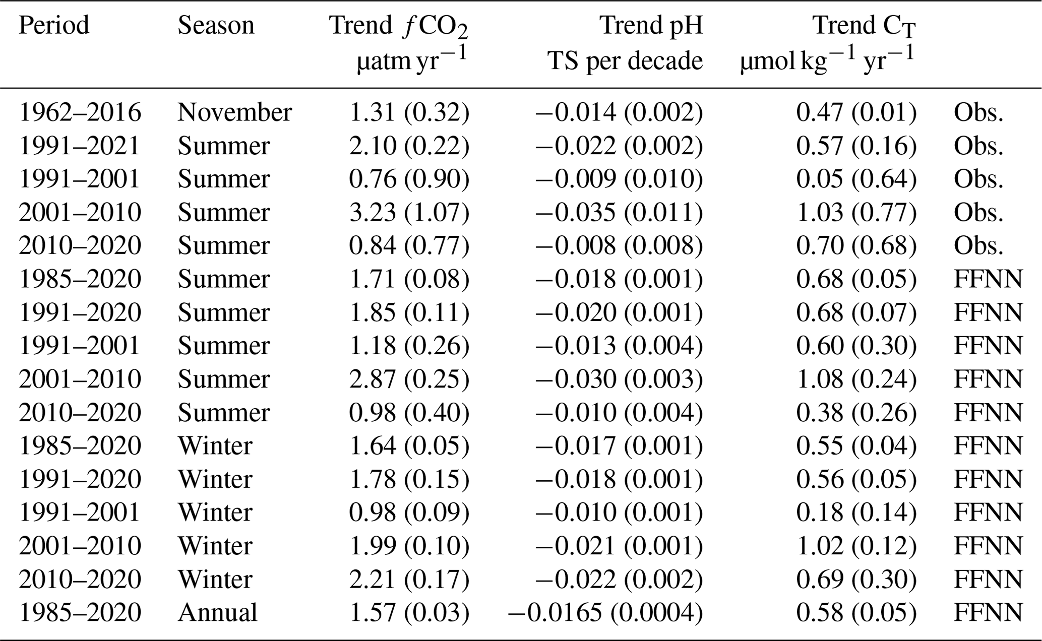
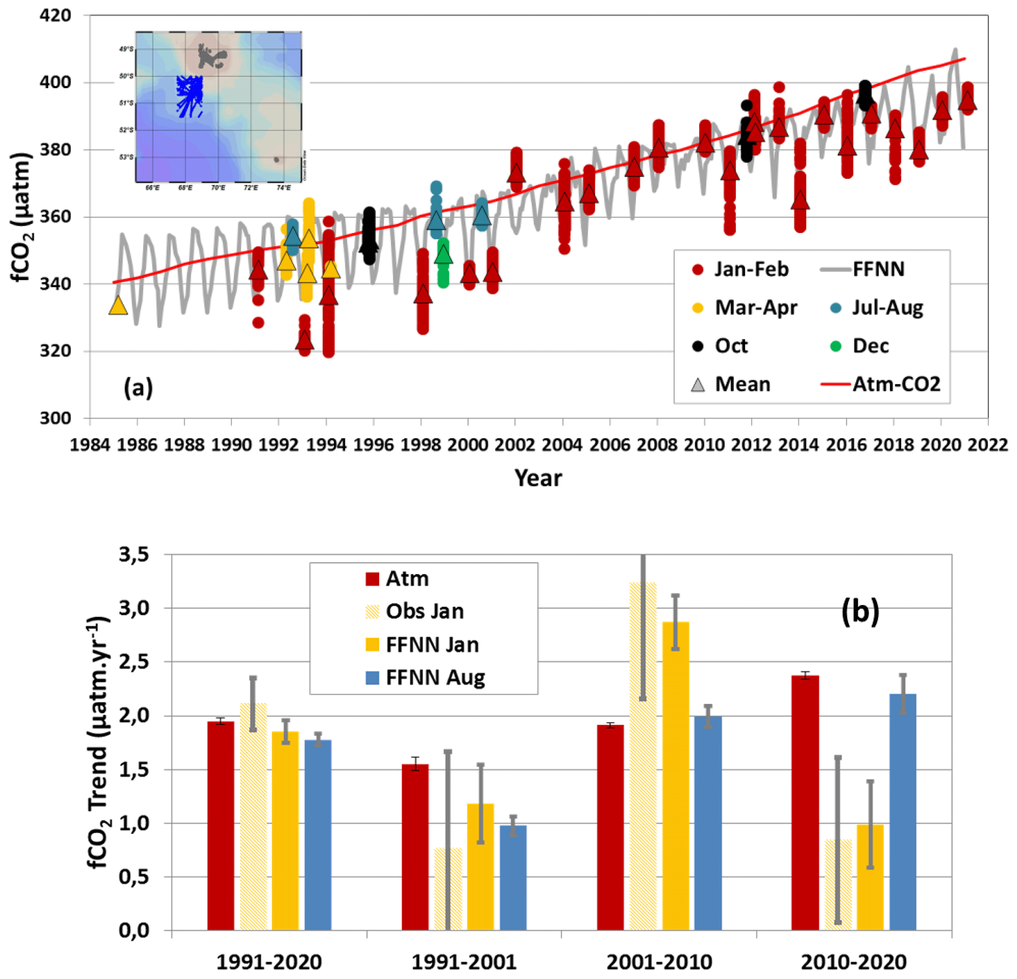
Figure 2(a) Time series of sea surface fCO2 observations (µatm) southwest of Kerguelen Islands in 1985–2021 (inset map shows the location of observations selected around station OISO-KERFIX at 50°40′ S–68°25′ E). The color dots correspond to five periods of the year (January–February, March–April, July–August, October, and December), and triangles show the average for each month. The monthly sea surface fCO2 from the FFNN model is presented for the period 1985–2020 (grey line), and the atmospheric fCO2 is represented by the red line. In March 1985 there was no underway fCO2 observation, and the triangle corresponds to fCO2 calculated with AT and CT measured in the mixed layer. (b) Trends of atmospheric and oceanic fCO2 (µatm yr−1) in summer and winter over four different periods based on observations (January) and the FFNN model (January and August). Inset map produced with ODV (Schlitzer, 2018).
3.1 Variability and trend of sea surface fCO2 and air–sea CO2 fluxes: 1985–2021
The fCO2 observations around 50° S–68° E and their mean values for each cruise are shown in Fig. 2a. fCO2 measurements are available for different seasons since 1991, though most of them stem from austral summer (January–February). During austral summer, the ocean fCO2 was generally lower than in the atmosphere (i.e., the ocean was a CO2 sink), whereas from July to October it was near equilibrium. The same seasonal change is obtained from the FFNN model for the period 1991–2020 (Fig. 2a). The model also indicates that between 1985 and the mid-1990s the fCO2 during austral winter (May–September) was always higher than the atmospheric fCO2, leading to an annual CO2 source during this period (Fig. 3). In 1985 the oceanic fCO2 from the FFNN model was higher than in the atmosphere from March to October (Fig. S4), resulting in an annual CO2 source of +0.8 molC m−2 yr−1. The model estimates a decrease of the annual CO2 source until the end of the 1990s followed by an increase of the source over the following decade (Fig. 3). Around the year 2010, the annual CO2 flux was around +0.5 molC m−2 yr−1 and then decreased over the last decade to change into an annual CO2 sink that increased to reach −0.5 molC m−2 yr−1 in 2020. For this reason and given the data available since 1991, we evaluated the summer and winter trends in fCO2, CT, and pH from the FFNN model over the three periods 1991–2001, 2001–2010, and 2010–2020 and compared the summer trends with those deduced from observations (Table 2). The analysis of trends and their associated drivers for different seasons and periods will allow us to explore links with the variability of primary production and/or the Southern Annual Mode (SAM). Shifts from a negative to a positive SAM index (Fig. 3) may have strengthened the upwelling of deep waters and could therefore impact ocean properties throughout the water column including CT, nutrients, primary production, or pH (e.g., Lovenduski and Gruber, 2005; Lenton et al., 2009; Hauck et al., 2013; Hoppema et al., 2015; Pardo et al., 2017).
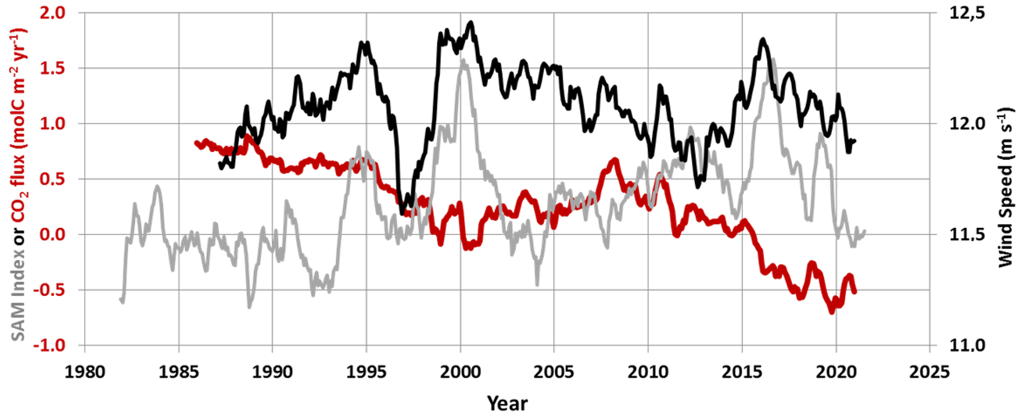
Figure 3Time series of the SAM index in the Southern Ocean (in grey), wind speed (in black, m s−1), and air–sea CO2 flux (molC m−2 yr−1) from the FFNN model (in red) at location 50.5° S–68.5° E. A positive (negative) flux represents a CO2 source (sink). Wind speed and SAM are presented for a 24-month running mean based on monthly values. Note the positive SAM (>0.5) in 1998–2002 and 2010–2019. SAM data from Marshall (2003), http://www.nerc-bas.ac.uk/icd/gjma/sam.html (last access: 14 August 2021). Wind speed data from ERA5 (Hersbach et al., 2020).
From the first underway measurements obtained at the OISO-KERFIX site in February 2021 to the last measurements used in this study in February 1991, the average oceanic fCO2 increased by +50.5 µatm (from 344.4±1.5 to 394.9±1.5 µatm; Fig. 2a). During the same period, the atmospheric CO2 increased by 57 µatm in this region (recorded at the Crozet Islands; Dlugokencky and Tans, 2022). This first comparison of two cruises 30 years apart indicates that the oceanic fCO2 increase was close to that of the atmosphere. During the same period, we observed small variations in AT (average µmol kg−1) and a clear increase in CT (Figs. 4a and S5). This suggests that most of the change observed in oceanic fCO2 and CT over the last 30 years is due to the uptake of anthropogenic CO2. However, the evolution of air–sea CO2 fluxes (Fig. 3) suggests that other mechanisms were at play over shorter periods, and changes in the air–sea fCO2 disequilibrium (Fig. 2a) suggest that different drivers may be involved in summer and in winter.
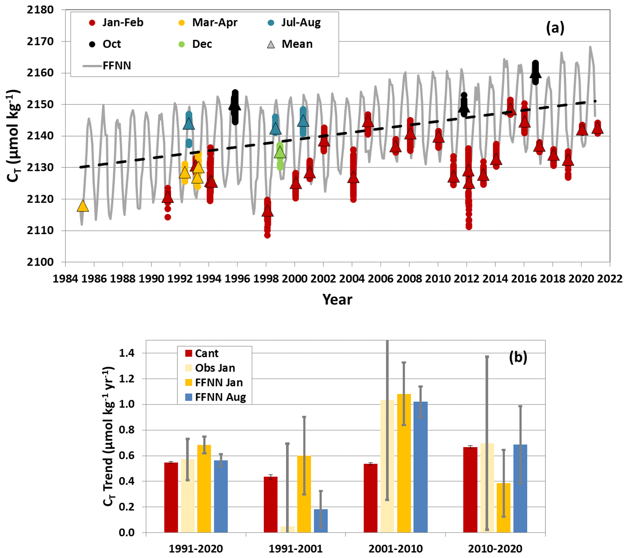
Figure 4(a) Time series of surface CT (µmol kg−1) around station OISO-KERFIX at 50°40′ S–68°25′ E calculated from fCO2 data (Fig. 2) using the AT–S relation (see Sect. 2.2.5). The color dots correspond to five periods of the year (January–February, March–April, July–August, October, and December), and triangles show the average for each month. The monthly sea surface CT from the FFNN model is presented for the period 1985–2020 (grey line). The annual CT trend of µmol kg−1 yr−1 (dashed line) is derived from the FFNN monthly data. In March 1985 the triangle corresponds to the observed CT in the mixed layer. (b) Trends of sea surface CT (µmol kg−1 yr−1) in summer and winter over four different periods based on observations (for January) and the FFNN model (for January and August). The trend for Cant (µmol kg−1 yr−1) is also shown (red bars) based on estimates in the winter water.
Summer data are characterized by a strong inter-annual variability in both fCO2 and CT (Figs. 2a and 4a) with the ocean being a CO2 source in January 2002, but a strong sink in January 1993, 1998, 2014, 2016, and 2019. In January 1998, when the surface ocean experienced a warm anomaly (Jabaud-Jan et al., 2004), the low fCO2 of 337 µatm and the low CT of 2110 µmol kg−1 (Figs. 4a and S5) co-occurred with intense primary production (Fig. 5), probably supported by diatoms as suggested by very low DSi concentrations (<2 µmol kg−1 down to 100 m, Fig. S6). In January 2014 and 2016, mixed-layer DSi concentrations were also remarkably small (<5 µmol kg−1 down to 75 m; Fig. S6). In 2014 low DSi coincided with Chl-a levels that started to increase in mid-November 2013 and stayed at a high level until February 2014 (surface Chl a >0.3 mg m−3; Figs. 5 and S7). The intense primary production contributed to the low fCO2 of 365 µatm reached by mid-January 2014, a value as low as 10 years earlier (Fig. 2a). To the contrary, in 2002 relatively low Chl a (mean Chl a <0.2 mg m−3; Fig. 5) was associated with higher levels of fCO2 (373 µatm), CT (2128 µmol kg−1; Figs. 4a, S5a), and DSi (Fig. S6). This was also associated with higher salinity indicative of entrainment that might be related to storm events that would have occurred few days before the measurements leading to brief positive fCO2 anomaly as recently observed from glider data in the subpolar South Atlantic (Nicholson et al., 2022). As opposed to the other periods the ocean was a source of CO2 in summer 2002 (this particular year was not well reconstructed by the FFNN model; Figs. 2a and S2b). The important inter-annual variability observed in summer indicates that in this region historically referred to as HNLC (Minas and Minas, 1992), primary production could significantly impact fCO2 levels in summer (Jabaud-Jan et al., 2004; Pasquer et al., 2015; Gregor et al., 2018), a result that needs to be taken into account when evaluating drivers of inter-annual variability (Rustogi et al., 2023) and the decadal trends of fCO2 or pH.
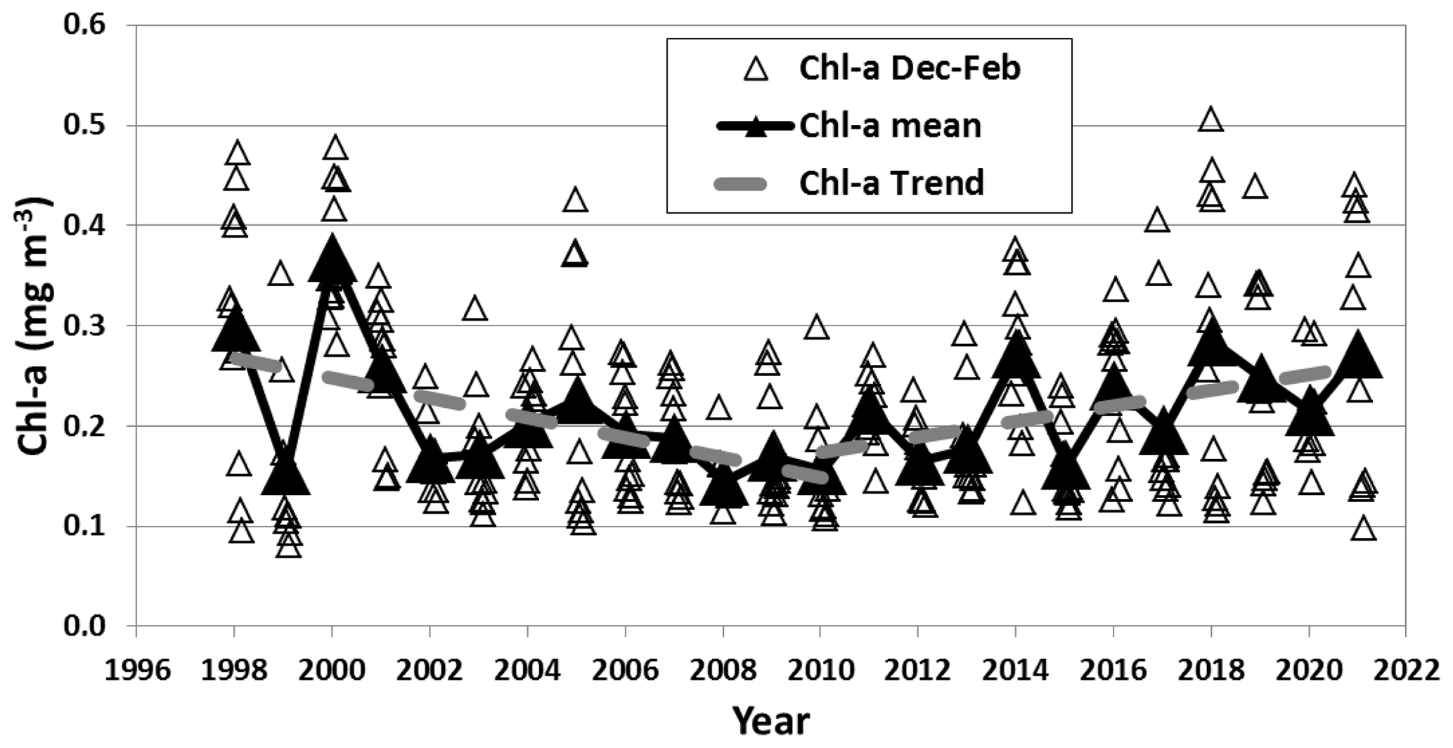
Figure 5Time series (1998–2021) of sea surface Chl a (mg m−3) in summer (December–February) from weekly satellite data (SeaWiFS and MODIS, open triangles) and associated mean (black triangles). The trends in 1998–2010 and 2010–2021 of respectively and mg m−3 yr−1 (dashed grey) indicate a decrease or increase of the primary production. The full Chl-a record is shown in Fig. S7.
The Chl-a time series derived from MODIS suggests higher concentrations in recent years compared to 2002–2013, with Chl-a peaks identified in 2014, 2016, 2018, 2019, and 2021 (Figs. 5 and S7) when the oceanic fCO2 in summer was well below the atmospheric level (Fig. 2a).
The primary production lowers CT concentrations and fCO2, i.e., opposite to the CT increase from anthropogenic CO2 uptake. These counteracting processes might explain the relatively stable fCO2 previously observed in the Indian POOZ in summer 2007–2019 with an annual fCO2 rate of increase of only µatm yr−1 (Leseurre et al., 2022). This low rate is confirmed here with the recent data obtained in 2020–2021 (Figs. 2b and S8). For the period 2010–2021, the oceanic fCO2 trend in summer derived from observations and the FFNN model is lower than +1 µatm yr−1 (Table 2), i.e., much lower than the atmospheric fCO2 rate of +2.4 µatm yr−1 and the oceanic fCO2 trend of µatm yr−1 estimated in winter by the FFNN model (Table 2, Fig. 2b). This rate is also lower compared to the change observed in October (+2.9 µatm yr−1) albeit being only based on two cruises in October 2011 and 2016 (Fig. 2a). As the low fCO2 trend in recent years is detected for summer only this is likely linked to an increase in primary production, as suggested by Chl-a records (Fig. 5). From 1998 to 2010 the summer Chl-a concentrations decreased at a rate of mg m−3 per decade, whereas from 2020 to 2021 Chl a increased by mg m−3 per decade (Fig. 5). These trends are coherent with previous studies, e.g., the reduced net primary productivity reported in the Indian Antarctic zone over 1997–2007 (e.g., Arrigo et al., 2008; Takao et al., 2012) and the shift of the Chl-a trend in 2010 also reported at large scale in the HNLC region of the Southern Ocean (Basterretxea et al., 2023). As a consequence, after 2010 the difference between oceanic and atmospheric fCO2 (ΔfCO2= fCO–fCO) decreased in summer (−1.4 µatm yr−1), and as it remains relatively steady during winter, the annual CO2 flux progressively varied from a source of +0.45 molC m−2 yr−1 in 2010 to a sink of −0.63 molC m−2 yr−1 in 2020 (Fig. 3). In addition, as the wind speed was stable during this period (12.0±0.9 m s−1 on average in 2010–2020; Fig. 3), the variation of the air–sea CO2 flux was mainly controlled by ΔfCO2 (e.g., Gu et al., 2023), and the decadal variation of primary production imprinted a significant change on the fCO2 trend and air–sea CO2 flux in this HNLC region. In the region investigated here, increasing Chl-a levels co-occurred with shifts of the SAM index to a positive state (Fig. 3), a link previously suggested south of the polar front in the SO but for a short period over 1997–2004 (Lovenduski and Gruber, 2005). Modeling studies also suggest that summertime biological activity could play an important role for the variability of the CO2 sink in the SO in response to the SAM (Hauck et al., 2013).
Another process to take into account for interpreting fCO2 trends is the change in temperature in surface waters. Previous analysis suggested a progressive warming in the region investigated here (Auger et al., 2021 for summer 1993–2017). Over 1998–2019 Leseurre et al. (2022) estimated a warming of Indian POOZ surface waters of °C yr−1. Extending the time series for the period 1991–2021 (Fig. S9a), we note that the surface temperature presents sub-decadal variability and that the ocean cooled after 2018 with a trend of °C yr−1 over 2018–2021 based on the monthly sea surface temperature (SST, Fig. S9b). The trend derived from our in situ observations in summer over this period was °C yr−1.
In 2019, the lower temperature and relatively high Chl a led to low fCO2 (380 µatm, Fig. 2a) and low CT (2128 µmol kg−1) compared to 2018 (fCO2=386 µatm; CT=2137 µmol kg−1, Fig. 4a). The decrease in observed fCO2 from summer 2018 to 2019, also reconstructed by the FFNN model (Fig. 2a), is contrary to the expected fCO2 and CT increase due to anthropogenic uptake. In 2020, although the temperature was also lower than in 2019, the oceanic fCO2 was higher (392 µatm) probably due to lower primary production as suggested by higher DSi (Fig. S6), as well as from CT (2135 µmol kg−1, Fig. 4a) and Chl-a records (Fig. 5). In January 2021 the temperature was close to that in January 2020, and both fCO2 and CT were slightly higher (395 µatm, 2139 µmol kg−1). AT concentrations were stable between 2018 and 2021 (2278.9±1.8 µmol kg−1, Fig. S5), indicating no effect of AT on the observed fCO2 change in this region as opposed to the areas north of the polar front in the Indian Ocean where AT variations are often linked to coccolithophore blooms (Balch et al., 2016; Smith et al., 2017).
The inter-annual and pluri-annual variability observed over 1991–2021 highlights the competitive processes that drive CT, fCO2, or pH temporal variations. In order to separate natural and anthropogenic contributions, the anthropogenic CO2 signal is estimated in the following section.
3.2 Anthropogenic CO2
3.2.1 Anthropogenic CO2 in the water column
To calculate anthropogenic CO2 concentrations (Cant), we used the TrOCA method developed by Touratier et al. (2007) and previously applied in the southern Indian Ocean (Mahieu et al., 2020; Leseurre et al., 2022). Such an indirect method is not suitable for evaluating Cant concentrations in surface waters due to biological activity and gas exchange, and we restrict the Cant calculations below the productive layer around 150 m. In the region south of the polar front, a well-defined subsurface temperature minimum is observed each year characterizing the winter water (WW) at a depth range of 150–250 m (Fig. 6a).
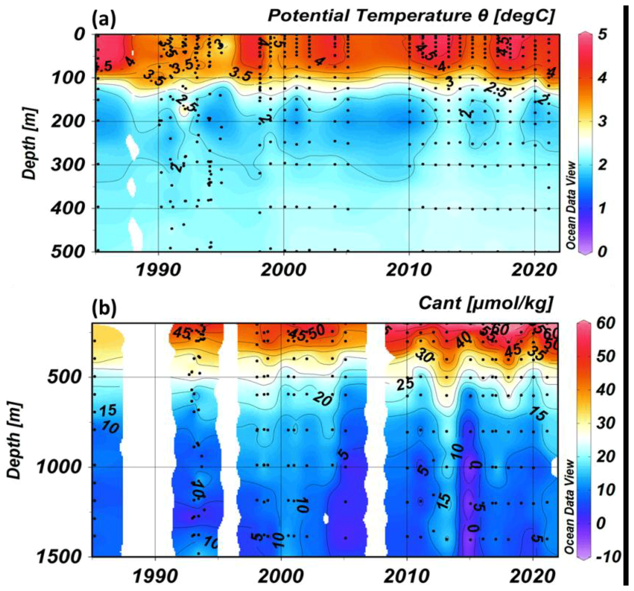
Figure 6Hovmöller section (depth–time) of (a) potential temperature (°C) and (b) anthropogenic CO2 (Cant, µmol kg−1) over 1985–2021 at station OISO-KERFIX (50°40′ S–68°25′ E). The section for temperature is presented in the layer 0–500 m and for summer to highlight the temperature minimum around 200 m (winter water, WW). The section for Cant is limited below 200 m. Section produced with ODV (Schlitzer, 2018).
The CT and Cant concentrations increased over time in the water column, a signal that is most pronounced in the top layers (200–400 m, Fig. 6b). In the deep layer, the presence of the Indo-Pacific Deep Water (IPDW) around 600–800 m is identified by a maximum of CT (CT>2250 µmol kg−1) and a minimum of O2 (O2 close to or <180 µmol kg−1, Fig. S10) (Talley, 2013; Chen et al., 2022). In the IPDW layer restricted to the neutral density (ND) range 27.75–27.85 kg m−3, there is no significant change in CT over time (Fig. S10). In that layer the Cant concentrations in 1985 (17.3 µmol kg−1) were almost identical to those evaluated in 2021 (21.2 µmol kg−1), considering the uncertainty in the Cant calculations (±6.5 µmol kg−1; Touratier et al., 2007). Below 800 m, the Cant concentrations were small but not null (Fig. 6b). The average Cant concentration below 800 m for all years and seasons was 8.0±5.3 µmol kg−1 (n=123) with a very small change detected over time (C µmol kg−1 in 1985 and C µmol kg−1 in 2021). As discussed above (Sect. 2.2.3) the CT and AT concentrations in the bottom layer (>1450 m) were stable over 1985–2021 (Table S2, Fig. S1).
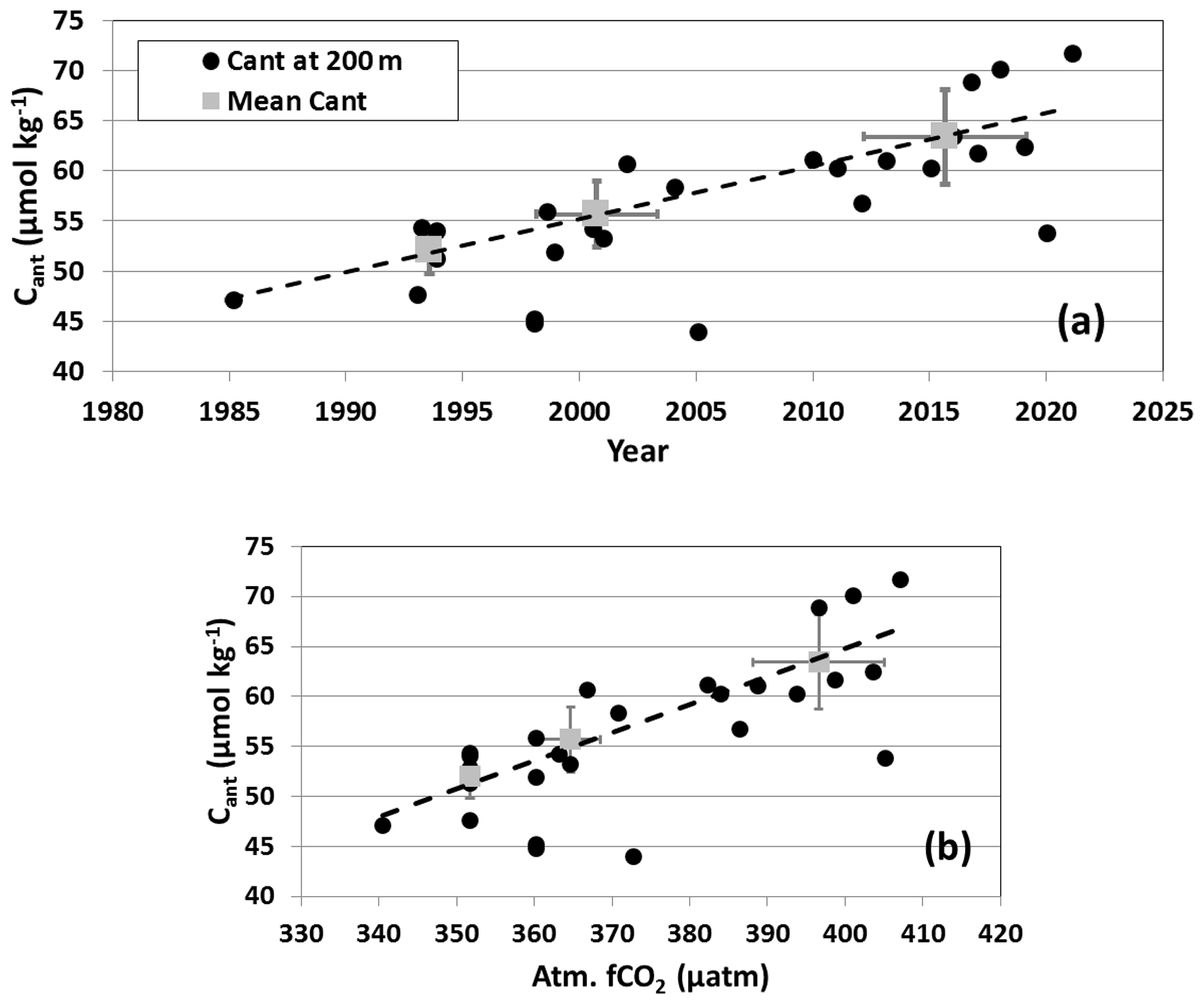
Figure 7(a) Time series of anthropogenic CO2 (Cant µmol kg−1) estimated in the winter water layer (WW around 200 m; see Fig. 6) from 1985 to 2021 at station OISO-KERFIX (50°40′ S–68° 25′ E). Black dots are the individual data in the WW and the grey squares the average for the 1990s, 2000s, and 2010s (anomalies in 1998, 2005, and 2020 discarded). The Cant trend of µmol kg−1 yr−1 is represented (dashed line). (b) Same data for Cant versus atmospheric fCO2 (the slope is µmol kg−1 µatm−1).
3.2.2 Anthropogenic CO2 trend in the winter water
To separate the natural and anthropogenic signals in surface waters for the driver analysis, we assume that Cant in the WW is representative of Cant in the mixed layer (ML). This is confirmed with few stations occupied during winter showing that Cant concentrations in the WW in summer are almost equal to Cant in the ML during the preceding winter (Fig. S11). The evolution of Cant in the WW from 1985 to 2021 is presented in Fig. 7a for all seasons. In 1985 the Cant concentration in the WW was 47.1 µmol kg−1, and Cant reached a maximum of 71.7 µmol kg−1 in 2021. The data selected at 200 m present some inter-annual variability such as the relatively low Cant in 1998, 2005, and 2020 probably related to natural variability. In 1998 and in 2020 the O2 concentrations were slightly lower in the WW (<300 µmol kg−1), explaining the lower Cant concentration (44.8 µmol kg−1 in 1998 and 53.8 µmol kg−1 in 2020), but no anomaly was observed for CT. This suggests that the biological contribution may have been overestimated (lower O2 is interpreted by the TrOCA method as more organic matter remineralization which should be associated with higher CT). This could be instead related to a change in mixing or circulation. In 2005 anomalies of CT, AT, and O2 concur to explain the lower Cant (43.9 µmol kg−1).
From 1985 to 2021, we estimated a Cant trend in WW of µmol kg−1 yr−1. When the Cant anomalies in 1998, 2005, and 2020 were discarded, this Cant trend was µmol kg−1 yr−1 (Fig. 7a). As expected, the Cant concentrations in the ocean are positively related to atmospheric CO2 (slope µmol kg−1 µatm−1; Fig. 7b). Interestingly, the slope observed south of the PF in the Indian Ocean is close to that observed in the Antarctic Intermediate Water (AAIW) in the South Atlantic ( µmol kg−1 µatm−1; Fontela et al., 2021). Gruber et al. (2019a, b) evaluated Cant changes between 1994 and 2007 in the global ocean. In the southern Indian sector, they estimated a mean Cant accumulation at the surface of µmol kg−1 in the band 50–55° S south of the PF. At our station location (50–52° S, 68° E) in the layer 0–250 m, the Cant accumulated from 1994 to 2007 was µmol kg−1. In 13 years, this corresponds to a trend of µmol kg−1 yr−1. Gruber et al. (2019a, b) did not use the data presented here, allowing for an independent comparison to the present study. Estimates of Cant accumulation by Gruber et al. (2019a, b) are in agreement with ours for the period 1994–2007 ( µmol kg−1 yr−1) but lower than reported here in recent years ( µmol kg−1 yr−1 over 2008–2021). Indeed our estimates over 3 decades indicate an increase in the uptake of anthropogenic CO2 with time (Fig. 4b).
3.2.3 Anthropogenic and surface CT seasonal trends
The Cant trend in the WW over 1985–2021 ( µmol kg−1 yr−1) is slightly lower than the annual surface CT trend derived from the FFNN model for 1985–2020 ( µmol kg−1 yr−1; Fig. 4a, Table 2) suggesting that anthropogenic CO2 uptake explains 86 % of the CT increase in surface waters. Over 1991–2020 the surface CT trend appears slightly higher in January than in August (Fig. 4b, Table 2). This suggests that in addition to the increase of CT due to anthropogenic CO2, other processes such as the variability of the biological activity, vertical mixing, or upwelling contributed to the observed trend. Indeed, as for fCO2 (Fig. 2b), the CT growth rate also depends on seasons and decades (Fig. 4b). Over 1991–2001 the CT trend from the observations ( µmol kg−1 yr−1; Table 2) is highly uncertain due to few data and the large variability (Fig. 4a, b). The FFNN model showed that the CT trend in summer was faster than the trend in Cant (Fig. 4b), suggesting that natural processes would have increased CT. This could be explained by an increase in vertical mixing due to the increase in wind speed (Fig. 3). On the contrary, the winter CT trend was lower than the Cant trend estimated in subsurface waters (Fig. 4b).
Over 2001–2010 the CT trends were much faster than over the previous decade, and they were the same for both seasons (Fig. 4b, Table 2). For this decade the summer CT trends from the observations and the FFNN model are coherent. They were also twice the Cant rate in the WW, which could be explained by enhanced upwelling of CT-rich deep waters during this period after the SAM reached a high positive index (Fig. 3; Lenton and Matear, 2007; Le Quéré et al., 2007; Hauck et al., 2013). However, over this period we did not detect any clear change at depth for ocean properties (except for CT and Cant) that would support this assumption (enhanced upwelling). The rapid CT (and fCO2) trend for this decade is probably due to processes occurring at the surface (e.g., biological activity, as discussed later) rather than changes in the water column (vertical mixing or upwelling). Over the last decade CT trends were lower than over the previous one (Fig. 4b). For summer, this is identified from both observations and the FFNN model. In winter the CT trend (from FFNN) is close to Cant, indicative of the anthropogenic CO2 accumulation. The low CT trend at the surface in summer, about half the Cant trend, is likely due to the increase of primary production after 2010 as described above (Fig. 5). Thus, it appears that the impact of biological activity and its variability in summer could counteract that of anthropogenic CO2 and explain the low temporal change of the carbonate system at the surface in recent years.
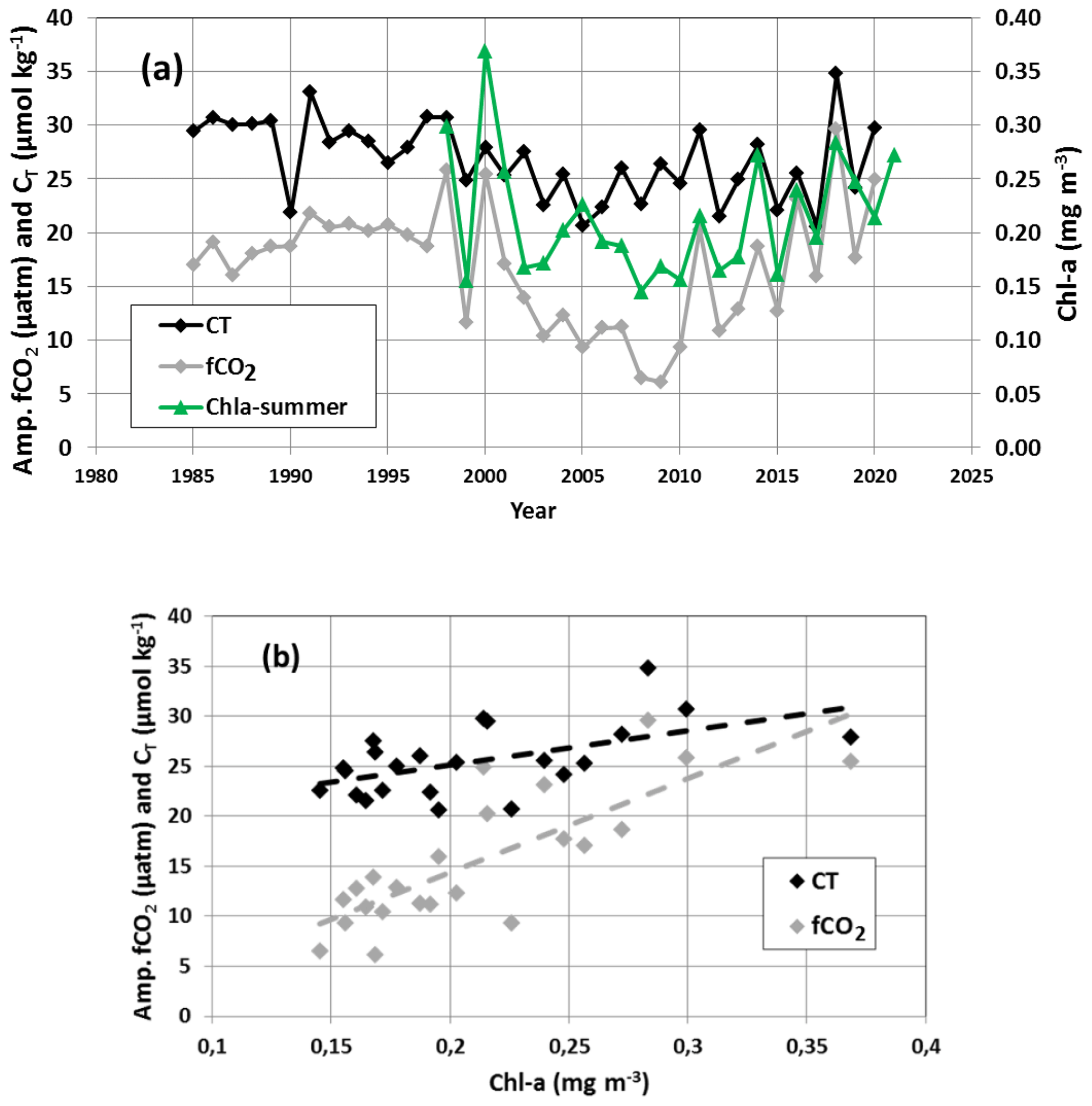
Figure 8(a) Time series of the seasonal amplitude (August minus January) for surface CT (black; µmol kg−1) and fCO2 (grey; µatm) from the FFNN model at station OISO-KERFIX (50°40′ S–68°25′ E). Also shown are the mean surface Chl a values (green; mg m−3) in summer from 1998 to 2021. (b) Seasonal amplitude of fCO2 and CT versus summer Chl a over 1998–2020. The dashed lines indicate that the seasonal amplitude (August–January) increases when Chl a is higher.
Given the differences of the fCO2 and CT trends in summer and winter (Figs. 2b and 4b, Table 2), we explored the temporal variations of the seasonality. For each year we estimated the differences between August and January (Fig. 8a). The seasonal amplitude for CT was on average 26.1±3.4 µmol kg−1 and for fCO2 15.1±5.6 µatm. Some large inter-annual variations appear related to the variability of Chl a in summer (Fig. 8a). Interestingly, the fCO2 seasonal amplitude reached a minimum around 2008–2010 and then increased over 2010–2020. This signal also appears correlated with the evolution of surface Chl a in summer (Fig. 8). This supports the conclusion that low phytoplanktonic biomass between 2008 and 2010 reduced the seasonal amplitude of fCO2.
The inter-annual variability of the seasonality is clearly identified when comparing CT with CT calculated due only to Cant accumulation (Fig. S12). This supports the conclusion that in addition to the Cant accumulation, the variations of phytoplanktonic biomass imprinted inter-annual variability on CT and fCO2 in summer. This holds for the seasonal amplitude as the results for winter follows the Cant trend (Figs. 4b, S12a). The same is true for pH for which reduced seasonal amplitude was found when the production was low (not shown). However, over 36 years (1985–2020) we did not identify a long-term trend of the seasonal amplitude for CT or for fCO2 as suggested by other studies (Landschützer et al., 2018; Rodgers et al., 2023; Shadwick et al., 2023). Our results highlight a variability over 5–10 years (Fig. 8a) and suggest a potential change in seasonality and annual CO2 sink if primary production changes in the future (e.g., Bopp et al., 2013; Leung et al., 2015; Fu et al., 2016; Kwiatkowski et al., 2020; Krumhardt et al., 2022; Seifert et al., 2023).
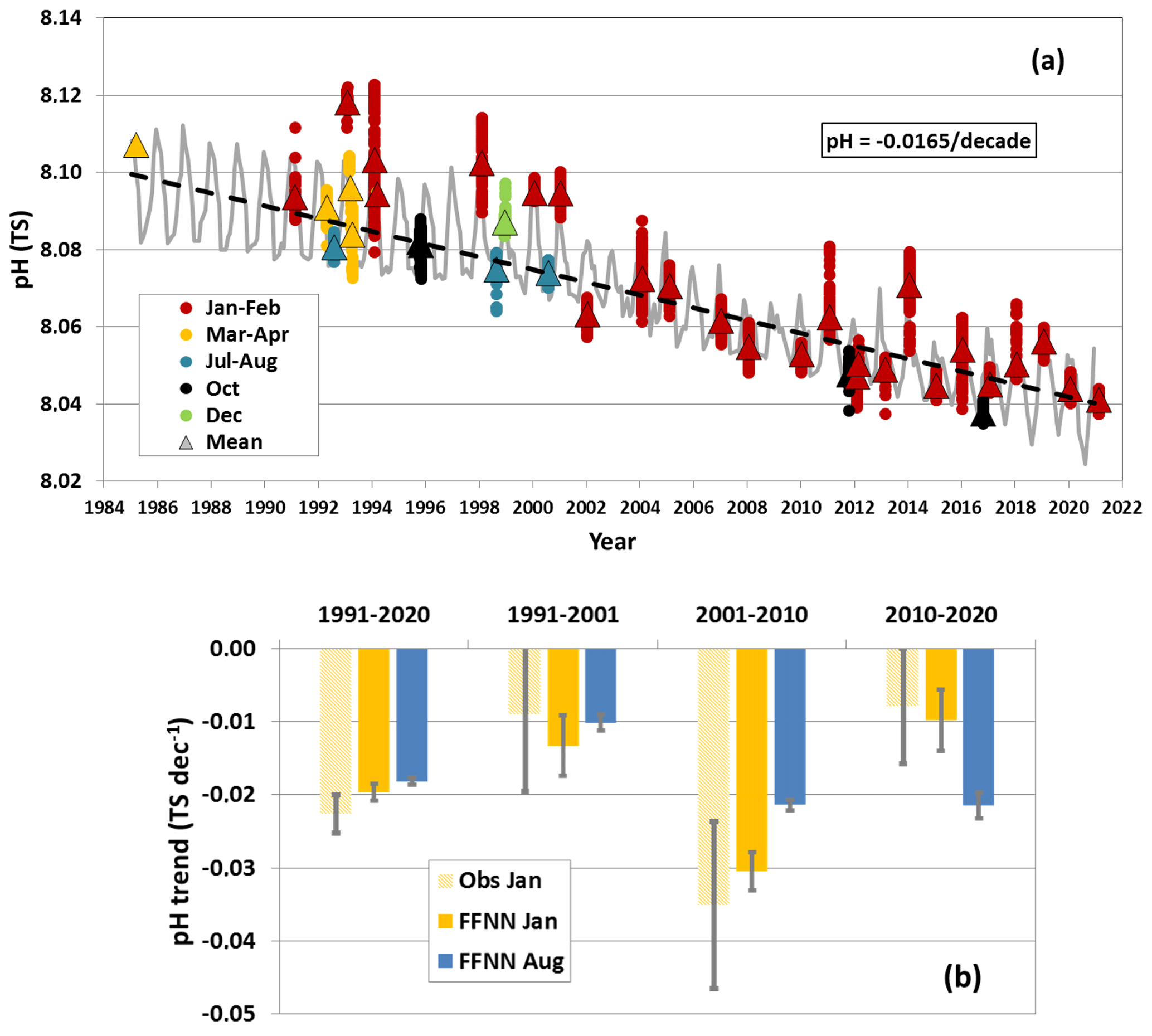
Figure 9(a) Time series of surface pH (total scale, TS) around station OISO-KERFIX(50°40′ S–68°25′ E) calculated from fCO2 data (Fig. 2) using the AT–S relation (see Sect. 2.2.5). The color dots correspond to five periods of the year (January–February, March–April, July–August, October, and December), and triangles show the average for each month. The monthly sea surface pH from the FFNN model is presented for the period 1985–2020 (grey line). The annual pH trend in 1985–2020 of per decade (dashed line) is derived from the FFNN monthly data (the same figure for [H+] concentrations is presented in Fig. S13). (b) Trends of pH (TS per decade) in summer and winter over four different periods based on observations (January) and the FFNN model (January and August).
3.3 Anthropogenic CO2 drives acidification in surface waters and in the water column
3.3.1 Surface pH trend
To explore the temporal change of pH in surface waters, we used the fCO2 observations and the monthly results from the FFNN model. For both datasets pH was calculated from fCO2 and AT reconstructed as described in Sect. 2.2.5. Figure 9a presents the time series of pH at the surface (the same time series for [H+] concentrations is shown in Fig. S13). For the full period, 1985–2020, the annual pH trend derived from the FFNN model is per decade (Table 2), exactly the same as derived at large scale in the Southern Ocean (south of 44° S) for the period 1993–2018 (Iida et al., 2021, Table 1), but when restricted to this period, 1993–2018, the trend from the FFNN model appears slightly faster ( per decade). This is less than the pH trend derived from pCO2 data in the SO subpolar seasonally stratified biome around 40–50° S (SO-SPSS) for 1981–2011 ( per decade; Table 1; Lauvset et al., 2015) and close to the pH trend based on OceanSODA-ETH reconstructed fields in the SO-SPSS for the period 1982–2021 ( per decade; Ma et al., 2023). However, as for fCO2 and CT, we estimated different pH trends in summer and winter, depending on the periods (Fig. 9b, Table 2).
The winter pH decrease estimated over the last 2 decades was twice as fast as estimated during the previous one, mirroring the winter fCO2 trends (Table 2). In summer, the pH trend presents a large variability at decadal scale as it was 3 times faster over 2001–2010 than during the previous and following decades (Fig. 9b, Table 2). Although the trends based on the observations are less robust because the cruises were not conducted each year, the reduced pH trend in summer after 2010 is confirmed from in situ data (Fig. 9b, Table 2).
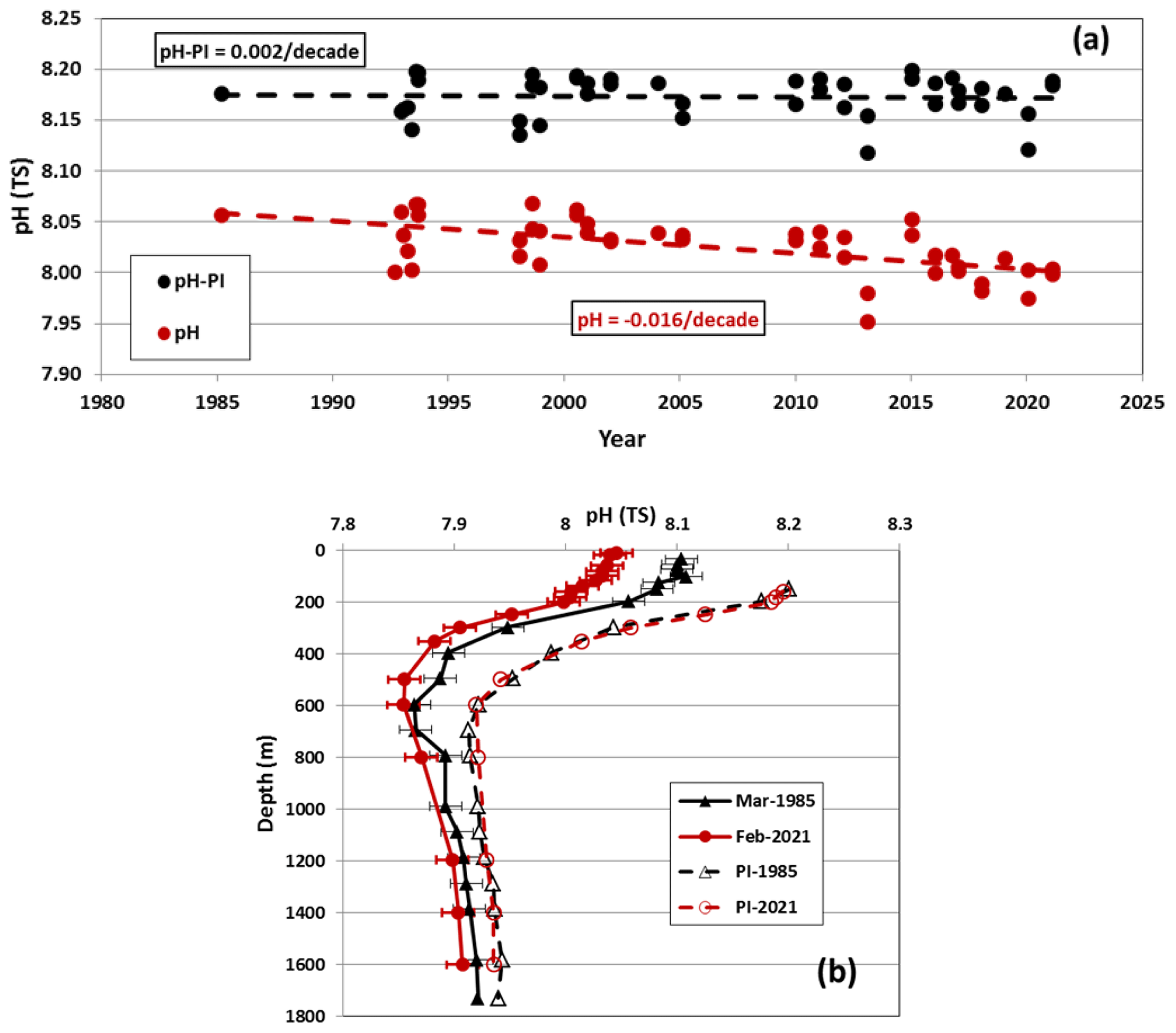
Figure 10(a) Time series of pH (red dots) and pre-industrial pH (pH-PI; black dots) estimated in the winter water layer (WW around 200 m; see Fig. 6) over 1985–2021 at station OISO-KERFIX (50°40′ S–68°25′ E). pH-PI for each sample was calculated after subtracting Cant to CT. The pH trend from the present day is per decade (dashed red line). No trend is observed for pH-PI (dashed black). The mean pH-PI in the WW is 8.173±0.020 (n=45). (b) Profiles of pH and pH-PI evaluated from March 1985 (black symbols) and February 2021 data (red symbols). The profiles for pH-PI are shown below 150 m only as Cant estimates are not available in the surface layer. Note that the pH-PI profiles are the same either using either the 1985 or 2021 data.
Our results show that the pH trend varied significantly from decade to decade and that part of the variations could be explained by the evolution of phytoplanktonic biomass, but overall the decrease of pH since 1985 was mainly driven by the accumulation of anthropogenic CO2. This is revealed in the winter water when comparing pH and pre-industrial pH (Fig. 10a). Here, the pre-industrial pH (pH-PI) was calculated after subtracting Cant values from the observed CT concentrations for each sample in the WW layer. Interestingly, the pH trend in the WW of per decade (here deduced from the station AT and CT data over 1985–2021) is very close to the annual trend at the surface deduced from the FFNN model over 1985–2020 ( per decade). This trend is slightly faster than the pH trends of per decade recently estimated in subsurface waters (100–210 m) of the Southern Ocean south of the PF and derived for years 1994–2017 from historical data and BGC-Argo floats (Mazloff et al., 2023). For the same period, 1994–2017, at the OISO-KERFIX station we estimated a pH trend in the WW of and of per decade in surface waters from the FFNN model.
As for other properties (AT, O2, temperature, salinity, and nutrients), the pre-industrial pH (pH-PI) does not change over time in the WW (mean pH-PI , n=45; Fig. 10a). The pH-PI in the WW is in the range of the pre-industrial surface pH value in the Southern Ocean (8.2 for year 1750 and 8.18 for year 1850) derived from Earth system models (Jiang et al., 2023, their Table S9). In the WW at our location the modern pH (1985–2021) was on average lower than pre-industrial pH. In 1985 pH in the WW was −0.119 lower than pH-PI, and in 2021 it was −0.184 lower than pH-PI (Fig. 10a). The progressive decrease of pH was clearly linked to Cant concentrations in the WW layer and the pH decrease identified below that layer in the water column (Fig. 10b).
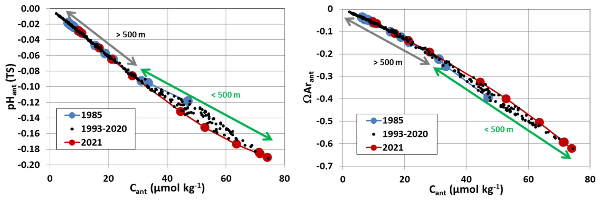
Figure 11Anthropogenic pH (pHant) and anthropogenic ΩAr (ΩArant) versus anthropogenic CO2 concentrations (Cant, µmol kg−1) at station OISO-KERFIX (50°40′ S–68° 25′ E). The data are selected in the layer 150–1600 m for the periods 1985 (blue), 1993–2020 (black), and 2021 (red). The green arrow identifies the data in the layer 150–500 m (for Cant>30 µmol kg−1). Below 500 m (brown arrow) no change of Cant was observed from 1985 to 2021 and thus for pHant and ΩArant.
3.3.2 Temporal change in the water column
From 1985 to 2021, signals of decreasing pH and increasing CT in surface waters are propagated in the water column down to about 500 m. As mentioned above the data in 1985 (first occupation of the station) reveal significant Cant levels across the water column (Fig. 6b). Therefore the pH down to the bottom was already lower in 1985 than at pre-industrial times (Fig. 10b). However, the largest Cant increases were found in the top layers, and changes in pH from 1985 to 2021 were small below 500 m (Figs. 10b, S14). While observations for all years fall on a common linear relationship between Cant and pHant for depths greater than 500 m, the change in pH for a given level of Cant increases with time for layers shallower than 500 m (Fig. 11).
The increase in Cant concentrations over time (Fig. 6b) also leads to a decrease of carbonate ion concentrations [CO] and of ΩAr and ΩCa (Figs. S14, S15). These decreases are well identified since the pre-industrial era in the whole water column, but in the last 36 years observations do not show any appreciable changes below 500 m (Fig. 11). The aragonite saturation horizon (ΩAr=1) was found around 600 m in 1985 and around 400 m in recent years (2015–2021; Figs. S14, S15). Moreover, during the period covered by observations (1985–2021), we did not detect abrupt change of the aragonite saturation horizon from one year to the next (nor between winter and summer; Fig. S16). This contrasts with previous regional studies in the SO and most notably with results from the layers close to the deep minimum of carbonate ion concentrations (Hauri et al., 2015; Negrete-Garcia et al., 2019). At our station the [CO] minimum lies around 500–600 m (Figs. S14, S15) and, along with the superimposed Cant accumulation, explains the upward shift of the aragonite and calcite saturation horizon between the pre-industrial and modern periods (Fig. S15). At pre-industrial time undersaturation with regard to aragonite (ΩAr <1) was found at the bottom only (1600 m), whereas between 1985 and 2021 it was found in the water column below 600 or 400 m (Fig. S15). The subsurface pre-industrial ΩAr value was around 1.9–2 (Fig. S15) and in the range of ΩAr value in the Southern Ocean at pre-industrial time from ESMs (Jiang et al., 2023, their Fig. 4).
The aragonite undersaturation already occurred in 1985 at 600–700 m, a layer corresponding to the [CO] minimum (Fig. S15), and a small increase of CT just above this layer (via Cant accumulation) would rapidly shift the aragonite saturation horizon above 600 m. This might have already occurred and could explain that ΩAr value was 1.02 at 350 m in 2021 (Fig. S15). These results suggest that for pelagic calcifiers living in subsurface waters (150 m or deeper) such as pteropods and foraminifera (e.g., Hunt et al., 2008; Meilland et al., 2018), the impact of acidification might occur sooner than at the surface.
For the interpretation of the trend analysis based on observations, only data below 150 m could be used as Cant was not evaluated in the surface layer. At 200 m, based on AT and CT data, we estimated a decrease in pH from 1985 to 2021 by −0.059 (Fig. 10b), corresponding to an increase by +1.1 nmol kg−1 in [H+] (Fig. S13) and a decrease by −0.16 in ΩAr (Fig. S15). Over 36 years, this represents about 30 % of the total change since the pre-industrial era for pH (−0.184), [H+] (+3.5 nmol kg−1), and ΩAr (−0.6). This is mainly linked to the Cant change that also represents over 36 years 30 % of the total accumulation (+24.6 µmol kg−1 from 1985 to 2021 for a total concentration of +71.7 µmol kg−1 at 200 m in 2021; Fig. 7). We conclude that the accumulation of anthropogenic CO2 drives the change of the carbonate system in subsurface waters and probably also in surface waters.
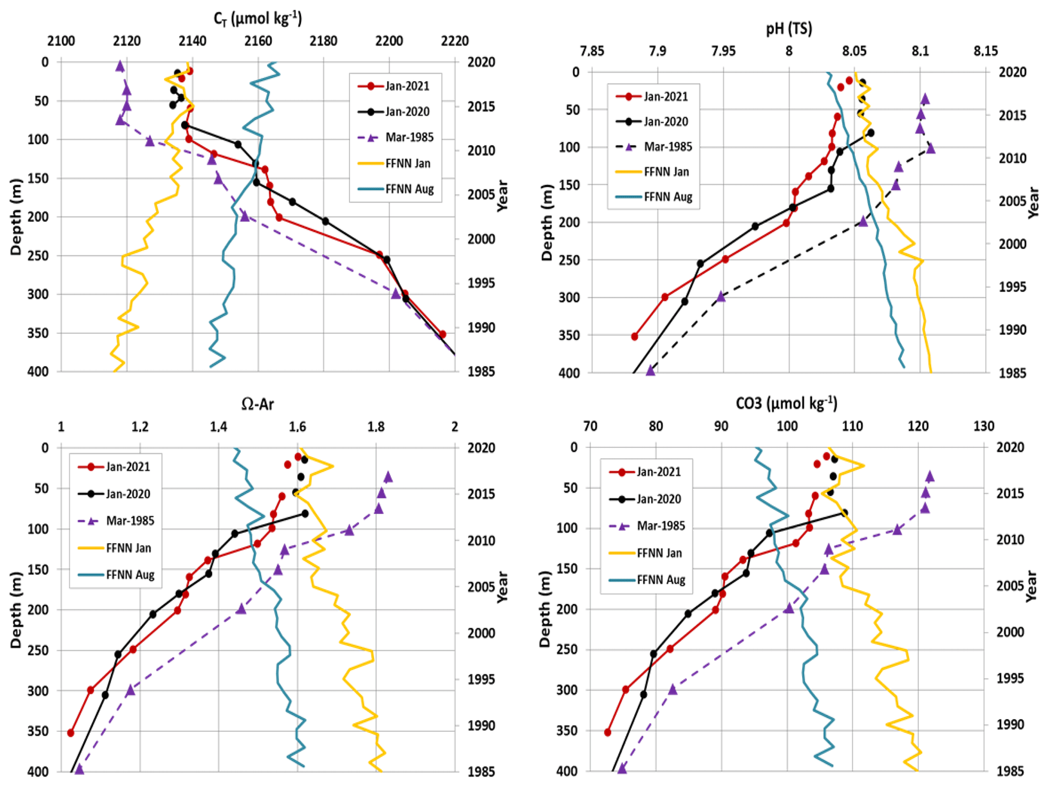
Figure 12Profiles (0–400 m, left axis) of observed and calculated properties (CT, pH, ΩAr, [CO]) at station OISO-KERFIX (50°40′ S–68°25′ E) in March 1985, January 2020, and January 2021 along with surface time series in 1985–2020 (right axis) of the same properties in January (yellow line) and August (blue line) from the FFNN model. The FFNN values in January 2020 are coherent with January 2020 or January 2021 observations in the mixed layer and in January 1985 are close to the observations in March 1985. Note that the differences of properties between 2020–2021 and 1985 have a similar magnitude as the seasonal amplitude (illustrated by the FFNN values for January and August).
In order to quantify the propagation of surface trends to depth, the temporal variations of carbonate system properties at the surface for both summer and winter derived from the FFNN model are compared to the changes observed across the water column (Fig. 12). The comparison shows that the seasonal amplitude of surface waters properties was of a similar magnitude to the observed changes in the mixed layer between 1985 and 2021. For example, the CT and ΩAr seasonal amplitude, respectively around 20 µmol kg−1 and 0.2, correspond to the CT increase and ΩAr decrease from 1985 to 2021. The comparisons also highlight that in summer the FFNN results were close to observations in the mixed layer (e.g., CT was 2120 µmol kg−1 in 1985 and 2140 µmol kg−1 in 2021). In winter, at the surface, CT was higher and pH, [CO], and ΩAr were lower (from the FFNN model; blue line in Fig. 12). The winter surface values in 1985 and 2020/2021 are in good agreement with observations at depth in the winter water (150–200 m). As an example, in 1985 surface CT in winter was 2145.5 µmol kg−1, which corresponds to the concentration measured at 150 m during summer (purple line in Fig. 12). In 2020, the winter CT at the surface (2168.3 µmol kg−1) is equal to CT concentrations observed at 150–180 m in January 2020 or in 2021. For ΩAr, the surface value derived from the FFNN model in winter 1985 (1.6) was equal to the ΩAr observed at 125 m in March 1985. In 2020, the surface winter estimate of ΩAr (1.42) was equal to ΩAr observed at 100–150 m in January 2020 or 2021. The same correspondences between winter surface and WW data were identified for pH and [CO] (Fig. 12). This supports the use of winter and summer surface data from the FFNN model to investigate the seasonal ΩAr trends and their projection in the future.
The surface water ΩAr (ΩCa) trend from the FFNN model in summer of −0.0059 yr−1 (−0.0094 yr−1) was stronger than the winter of −0.0050 yr−1 (−0.0079 yr−1) and also higher than the trend derived from observations in the WW (−0.0043 yr−1 for ΩAr and −0.0069 yr−1 for ΩCa). Our results indicate that the change of carbonate properties in the years 1985–2021 were mainly driven by Cant accumulation in surface waters and across the water column. However, a potential increase in primary productivity after 2010 mitigated the effects of increasing Cant accumulation in response to increasing atmospheric CO2 leading to relatively stable summer CT and fCO2 and to a stronger CO2 sink (Fig. 3). Consequently, when restricted to the period 2010–2020, the trend of ΩAr in surface waters in summer was much smaller, per decade than during the preceding period. This was much smaller than derived from all the data over 1985–2021 (−0.048 per decade) or estimated from reconstructed fields in the SO-SPSS over 1982–2021 (−0.0616 per decade; Ma et al., 2023). It underscores the uncertainty in extrapolating time series to the future depending on the selection of data and periods.
3.4 Long-term change in surface water: from the 1960s to the future
The data described above allowed evaluating the temporal variations of the properties of the carbonate system and Cant over 1985–2021 along with a comparison to the pre-industrial state in the water column. The results over 36 years informed on the recent changes, inter-annual variations, and trends, but the time series appears somehow short to extrapolate the trends over time. What was the change of the carbonate system in surface waters before 1985 and what will be its future evolution?
3.4.1 Back to the 1960s: observed trends since 1962
To explore the long-term change, we start by comparing our recent data with observations from the LUSIAD cruise conducted in 1962–1963 (Keeling and Waterman, 1968). Some data from this cruise were obtained in mid-November 1962 south of the polar front, in the region southwest off Kerguelen Islands. Because of the seasonality, we compared the November 1962 data with our observations obtained in October–November in 1995, 2011, and 2016 and with the FFNN model results for November (Fig. 13). The CT concentration, pH, ΩAr, and ΩCa for 1962 were calculated using fCO2 data and AT (from the AT–S relationship in Eq. 1) with salinity from the World Ocean Atlas (Antonov et al., 2006).
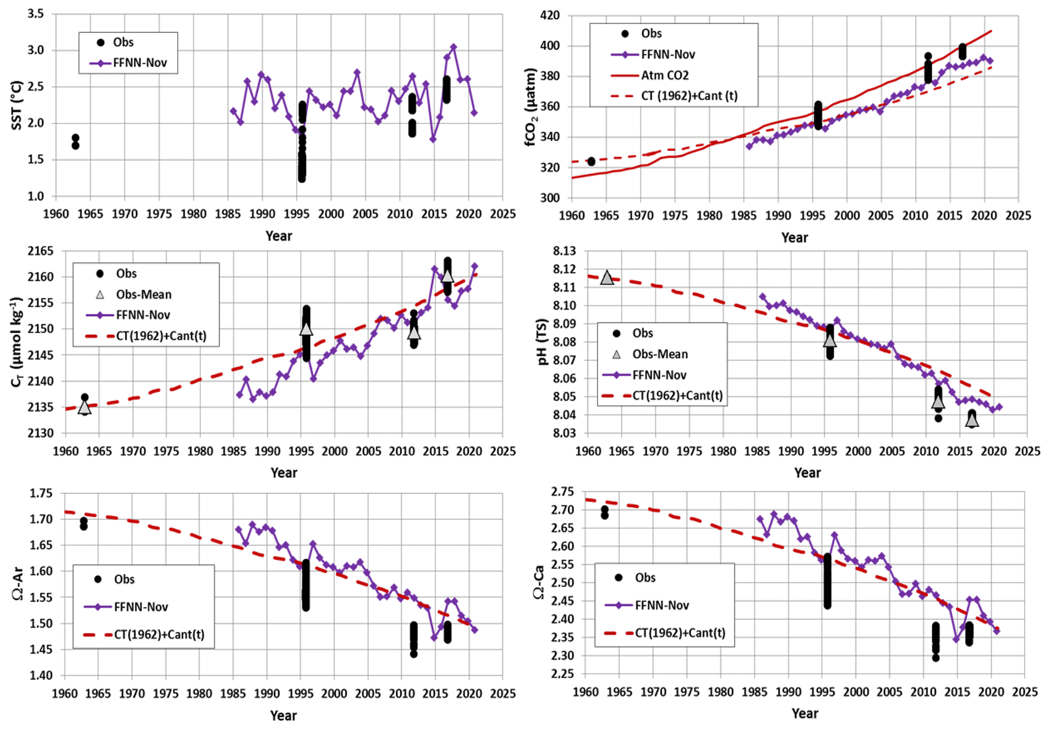
Figure 13Observed (black dots) sea surface temperature (°C), fCO2 (µatm), CT (µmol kg−1), pH (TS), ΩAr, and ΩCa around station OISO-KERFIX at 50°40′ S–68°25′ E for October–November. Also shown are the results for the FFNN model for November in 1985–2020 (purple). The CT concentrations, pH, ΩAr, and ΩCa were calculated from fCO2 data using the AT–S relation (Eq. 1). The red line is the atmospheric fCO2, and dashed red lines in each plot are the evolution of properties since 1960 corrected for Cant where fCO2, pH, ΩAr, and ΩCa were recalculated using CT+Cant, AT constant at 2290 µmol kg−1, and SST at 2 °C. Grey triangles identify the mean values for CT and pH.
First, we note that the measured SST in November 1962 (1.7 °C) was slightly lower compared to recent years (on average by about −0.6 °C), but SST as low as 1.8 °C for this season was also found in other years (e.g., November 1995, 2014). The change in SST is unlikely to explain the long-term increase in fCO2 or decrease in pH since 1962 (Fig. 13). In 1962, the oceanic fCO2 was 324 µatm, which is slightly higher than in the atmosphere (ΔfCO µatm, a small source), whereas in November 1985–2020 the ocean was a small CO2 sink on average (ΔfCO µatm). The CT concentration in 1962 (2135 µmol kg−1) was much lower than observed since 1995, and the pH (8.115) was much higher than in the last 3 decades (Fig. 13). Compared to 1962, pH in 2016 was −0.078 lower, i.e., representing 70 % of the pH decrease of −0.11 in the global ocean since the beginning of the industrial era (Jiang et al., 2019). In November 1962, surface CT was lower by −15.1 µmol kg−1 compared to the data in October 1995, i.e., a trend of +0.46 µmol kg−1 yr−1 over 33 years close to the Cant trend observed in the WW over 1985–2021 as described above ( µmol kg−1 yr−1). Having the CT value in 1962, we can project the CT in time by adding the Cant concentration based on the relationship observed between Cant and atmospheric CO2 (Fig. 7b) assuming that the anthropogenic CO2 uptake since the 1960s is representative of the CT change (i.e., the change of CT due to natural variability was small). This projection is shown for all properties (dashed red lines in Fig. 13) and confirms that the progressive Cant accumulation explained most of the CT and fCO2 increase in surface waters since 1962. We note that the CT derived from the FFNN model suggests slightly lower CT compared to the Cant projection especially before 2006. The difference of projected CT and the FFNN model (on average µmol kg−1) is within the uncertainty of CT calculations (error is ±5 µmol kg−1 when using the AT/fCO2 pairs), and the trend of the difference over 1985–2020 (−0.15 µmol kg−1 yr−1) is too small to be related with confidence to changes associated with natural processes. On the other hand, the oceanic fCO2 recalculated with the projected Cant trend suggested that for this season (November) the ocean moved from a CO2 source in 1962–1985 (ΔfCO2>0) to a sink in 1986–2021 (ΔfCO2<0) in line with results from the FFNN model. The recalculated fCO2 with Cant (dashed red line in Fig. 13) was close to that observed in 1995 or from the FFNN model in 1985–2014 (mean difference over 1985–2014 is µatm). After 2016, the recalculated fCO2 suggests a stronger sink, and the difference with observations in 2011 and 2016 or the FFNN model is slightly higher (mean difference over 2016–2020 is µatm). Although the differences are in the range of the error in fCO2 calculation using AT–CT pairs (±13 µatm), this might indicate that after 2016 a process could contribute to increase fCO2 faster than the effect of Cant only. This difference could be due to the warming that occurred after 2016 when SST was higher than 2 and up to 3 °C in November 2017 (Figs. 13 and S9). The same could be applied for pH that was slightly lower than the pH recalculated from Cant trend after 2015 (the mean difference between recalculated pH and FFNN-pH over 1985–2020 is only 0.002±0.006). Therefore, we conclude that for November the pH decrease since 1962 was mainly driven by the accumulation of anthropogenic CO2. Aragonite and calcite saturation states also show a clear decrease since 1962 (Fig. 13), a diminution of 11 % over 59 years for both ΩAr and ΩCa. Based on these results over almost 60 years that confirm the conclusions from the observations in 1985–2021, we now evaluate the long-term change of the carbonate system in surface waters in the future.
3.4.2 Projecting the observed trends in the future
The trends of the properties based on observations in 1962–2021 and the FFNN model in 1985–2020 indicate relatively linear trends linked to Cant uptake albeit with some decadal variability in summer (Fig. 4). A simple linear extrapolation of the trends in the future suggests that aragonite undersaturation in surface waters would be reached in year 2110 for the winter season and 2120 for summer (Fig. S17), whereas the subsurface trend suggests undersaturation in 2090. In year 2100, surface pH and [H+] would be around 7.9 and 12 nmol kg−1 (Fig. S17). However, ESM CMIP6 models suggest that under a high emission scenario (SSP5-8.5), pH in 2100 in the Southern Ocean near 50° S would be around 7.65 and [H+] around 22 nmol kg−1 (Jiang et al., 2023, their Fig. 4). This shows that the simple linear extrapolation based on recent observed trends (Fig. S17) underestimated the future change of the carbonate system for a high emission scenario as previously shown in the southeastern Indian Ocean based on summer trends derived from observations in 1969–2003 (Midorikawa et al., 2012, their Fig. 4).
Table 3Results of the simulated properties for year 2020, 2050, and 2100 for two emission scenarios (SSP5-8.5 and SSP2-4.5). For 2020 the results based on observations in January (Obs.) and the FFNN model in January and August also listed. Sensitivity tests: “SSP85 W-T” is for winter with constant temperature, and “SSP85 W-A-T” is for winter with constant AT and temperature.
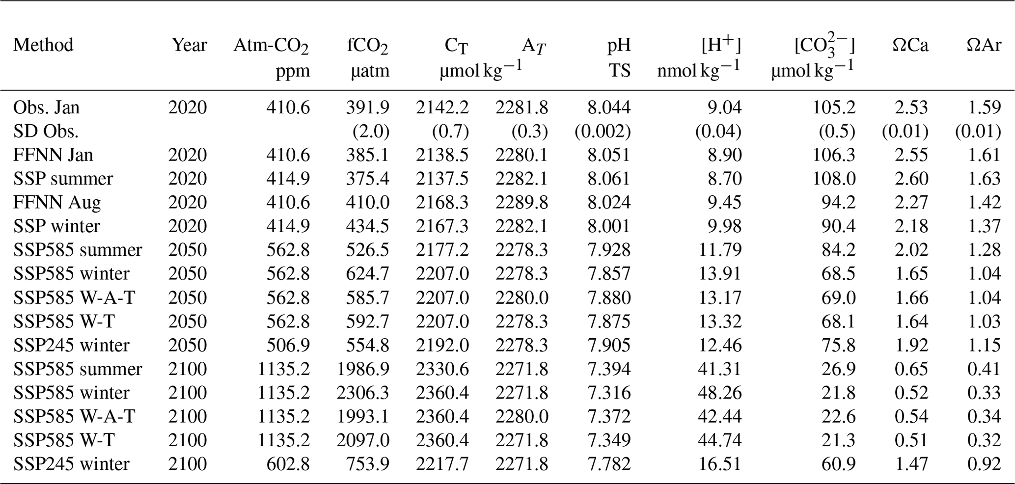
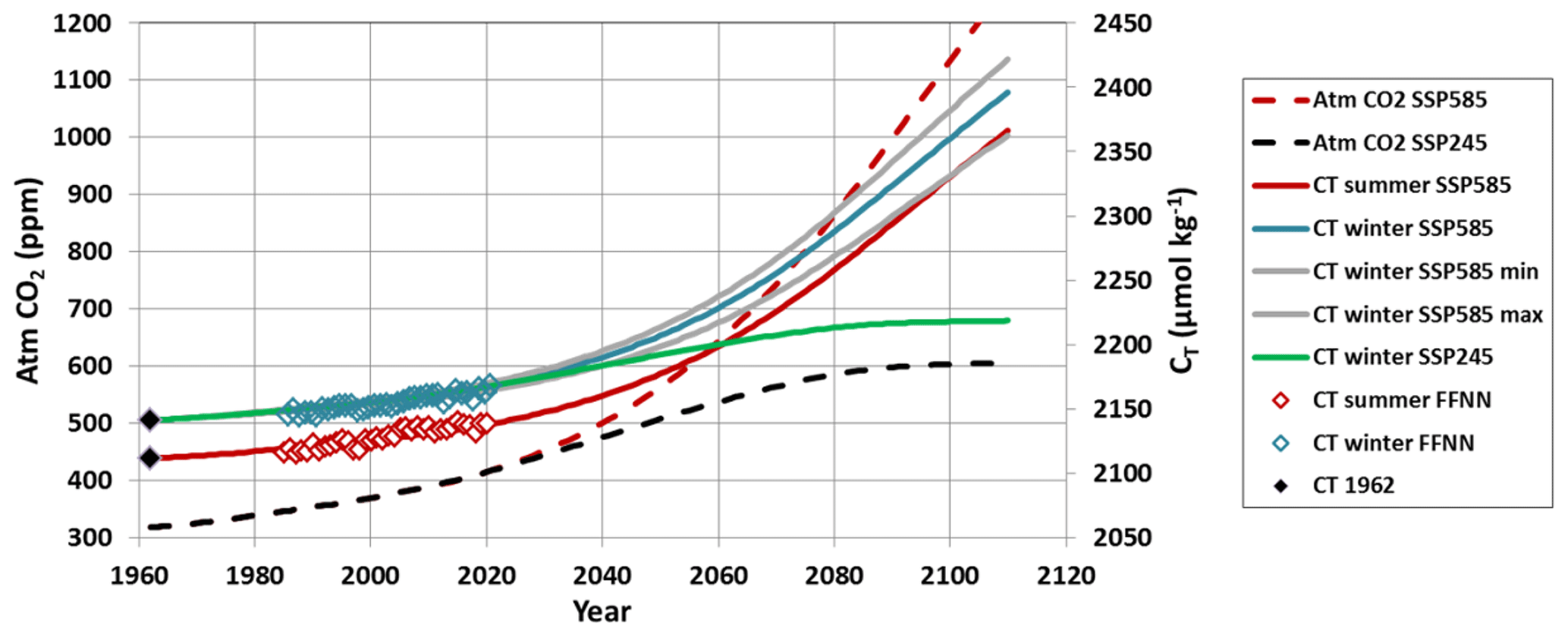
Figure 14Evolution of atmospheric CO2 (ppm) and sea surface CT (µmol kg−1) between 1960 and 2110 evaluated for two scenarios (SSP2-4.5 dashed black and SSP5-8.5 dashed red), for summer (red line for SSP5-8.5) and winter (blue line for SSP5-8.5 and green line for SSP2-4.5). Grey lines are the high and low CT for winter SSP5-8.5 based on the error in the Cant/fCO2 relationship (Fig. 7b). Also shown are the results for the FFNN model in 1985–2020 for summer (red diamonds) and winter (blue diamonds) and CT in 1962 (black diamonds). The CT values for different seasons and scenarios were used to calculate the carbonate properties in the future (Fig. 15).
To better investigate the changes for the next decades, we assumed that the Cant trend for the modern period (Fig. 7) that experienced a “business as usual” scenario after the 1960s is representative of the future changes in the surface ocean carbonate system. For this analysis, we used two emissions scenarios (shared socioeconomic pathways, SSPs; Meinshausen et al., 2020) with atmospheric xCO2 reaching 1135 ppm in 2100 (a “high” emission scenario SSP5-8.5) or xCO2 reaching 603 ppm in 2100 after a stabilization around 2080 (scenario SSP2-4.5). This enables us to simulate future CT concentrations for summer or winter (Fig. 14) and to calculate other carbonate properties using CT and AT (Fig. 15, Table 3) in response to approximated future changes in physical and geochemical properties excluding impacts of changes in atmospheric and oceanic circulation. As the calculated properties are sensitive to AT values, we used a fixed AT of 2280 µmol kg−1 or applied a correction based on the long-term change of sea surface salinity observed in the last 6 decades (1960–2017), i.e., a freshening in the Southern Ocean of around −0.01 to −0.02 per decade (Durack and Wijffels, 2010; Cheng et al., 2020b). The decrease in salinity in the southern Indian Ocean ( per decade) was recently analyzed by Akhoudas et al. (2023), who showed that in the years 1993–2021 the freshening was mainly due to an increase in precipitation linked to the acceleration of the atmospheric hydrological cycle. From our data in the mixed layer over 1985–2021, we estimated a trend in salinity of per decade. For the AT sensitivity test, we thus selected a salinity trend of −0.01 per decade in 1962–1985 and −0.02 per decade after 1985 and applied these trends to simulate AT over 1960–2100 using the AT–salinity relationship (Eq. 1). This leads to a salinity of 33.650 and AT of 2272 µmol kg−1 in the year 2100, about 8 µmol kg−1 lower than observed in 2021 (2280 µmol kg−1). Compared to the CT change from 2021 to 2100 (+50 and +193 µmol kg−1 for the “low” and “high” emissions scenario, Fig. 14), the impact of the AT decrease has a minor effect on the future change for pH, [CO], and Ω (Table 3). For example, in winter for the SSP5-8.5 scenario, when the AT decrease is taken into account, pH in 2100 is 7.316 and ΩAr is 0.33 against 7.372 and 0.34 when AT is constant (Table 3). In both cases, the surface aragonite undersaturation (ΩAr=1) in winter occurred in 2055, whereas in summer it is identified in 2070. The effect of lower AT in the future appeared also small compared to the seasonal differences of pH and Ω in 2100.
As noted above, the Southern Ocean experienced a warming in recent decades (e.g., Auger et al., 2021), and it is projected that warming will continue in the future (IPCC, 2022). Therefore, to test the sensitivity of calculated properties to warming we applied a warming of +0.0125 °C yr−1 in 1985–2020 and +0.025 °C yr−1 after 2020 (Azarian et al., 2023). As for AT, these results are compared for winter using constant SST (Table 3). The effect of the long-term warming does mainly impact the projection of [H+] and pH (Table 3).
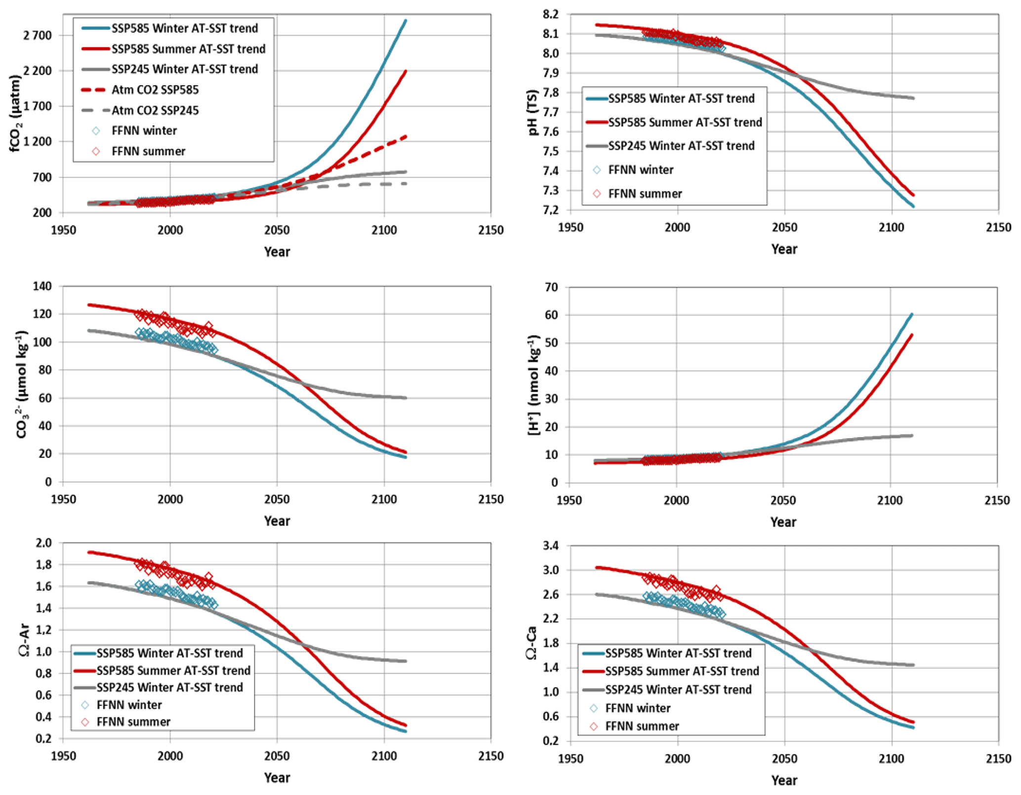
Figure 15Evolution of sea surface fCO2 (µatm), pH (TS), [CO] (µmol kg−1), [H+] (nmol kg−1), ΩAr, and ΩCa between 1960 and 2110 evaluated for the SSP5-8.5 scenario for winter (blue line) and summer (red line) taking into account both AT and SST future trends. For winter the results are also presented using the SSP2-4.5 scenario (grey lines). Also shown are the results for the FFNN model in 1985–2020 for summer (red diamonds) and winter (blue diamonds). Atmospheric fCO2 is also shown for SSP5-8.5 (dashed red) and SSP2-4.5 (dashed grey). Values in 2020, 2050, and 2100 for different sensitivity tests are listed in Table 3.
These sensitivity tests for temperature and AT showed that as for the observed period 1962–2021 (Fig. 13), the projection in the future depends mainly on the anthropogenic CO2 accumulation. Here, the CT concentrations were calculated using the Cant versus atmospheric CO2 relationship (Fig. 7b). We thus tested the results for winter based on the error associated with this relationship (Fig. S18). This leads to either higher or lower CT compared to the original calculation (Fig. 14). For the SSP5-8.5 scenario, the winter CT concentrations in 2100 range between 2328 and 2378 µmol kg−1, higher than simulated in the ESM CMIP6 models around 50° S (2300 µmol kg−1; Jiang et al., 2023). As in the ESMs, the projected CT concentration in 2100 at our location for the SSP2-4.5 scenario is much lower, 2217 µmol kg−1 (Fig. 14). The future change of the carbonate system is not significantly different using low or high Cant accumulation (Fig. S18), but this test gives a range of years to reach aragonite and calcite undersaturation. In winter (SSP5-8.5 scenario), aragonite (calcite) would reach undersaturation between year 2050 and 2060 (between year 2070 and 2080). Note that for summer we derived undersaturation for ΩAr in year 2065 and for ΩCa in year 2085. For the SSP2-4.5 scenario, where CT is 143 µmol kg−1 lower in 2100 compared to SSP5-8.5, aragonite undersaturation would not be reached before 2070 (Fig. 15).
The times series of high-quality observations collected between 1985 and 2021 and the results from the FFNN model at one location, south of the polar front in the southern Indian Ocean (50° S–68° E), presented in this analysis offered new results on the inter-annual variability, decadal to long-term trends of the carbonate system in surface waters, air–sea CO2 fluxes, and associated drivers. The evaluation of anthropogenic CO2 concentrations in the water column indicated that the trends of the carbonate species are mainly driven by the anthropogenic CO2 uptake leading to a progressive acidification in surface waters and at depth.
In 1985, the Cant concentrations were approaching 50 µmol kg−1 at 200 m, and Cant was detected in the water column down to the bottom (1600 m). This explains why aragonite undersaturation was observed at 600–700 m in 1985, where [CO] concentration was at its minimum, whereas for the pre-industrial era the whole water column was super-saturated (this study Fig. S15; Lauvset et al., 2020, their Fig. S15). Because of the anthropogenic CO2 accumulation, 36 years later, we observed an upward migration of the aragonite saturation horizon that was found around 400 m in 2021 (a shoaling rate of around −6 m yr−1).
At the subsurface, in the winter water layer, the Cant trend is estimated at µmol kg−1 yr−1 over 1985–2021 with a detectable increase of the trend in recent years. The Cant concentrations in the ocean are closely related to the atmospheric CO2 concentrations, and the slope we observed south of the PF in the Indian sector of µmol kg−1 µatm−1 is close to that observed in the AAIW in the South Atlantic (Fontela et al., 2021). This suggests that local observations in the southern Indian POOZ captured the link between Cant and atmospheric CO2 at a larger scale.
In surface waters, over 1991–2020 the oceanic fCO2 increased at a rate close to or slightly lower than in the atmosphere (Fig. 2b), and the CT trend followed the Cant accumulation (Figs. 4b, S12a). However in the last decade both observations and the FFNN model showed low fCO2 trends in summer (less than 1 µatm yr−1). The change in summer trend appears related to primary production as revealed by a decrease of Chl a in 1998–2010 followed by an increase after 2010. Biological activity counteracts the CT increase due to Cant, resulting in rather stable CT and fCO2 in summer during the last decade. As a result, the region moved from an annual source of +0.8 molC m−2 yr−1 in 1985 to a sink of −0.5 molC m−2 yr−1 in 2020. Adding historical data from November 1962 that indicate an annual source of 2.2 molC m−2 yr−1 and extrapolating to the entire southern Indian POOZ (50–58° S, 20–120° E; 6.5 M km2) suggest that this region changed from a CO2 source of 0.17 PgC yr−1 in 1962, reduced to 0.06 PgC yr−1 in 1985, to a CO2 sink of −0.04 PgC yr−1 in 2020. This can be compared with reconstructed fluxes from a data-based model that produced a CO2 source around 0.10 PgC yr−1 in 1960–1990 and a sink around −0.05 PgC yr−1 in 2020 in the southern Indian sector (Rödenbeck et al., 2022, their Fig. 6). Based on the FFNN reconstructions, the increase of the ocean CO2 sink was particularly pronounced after 2011 (Fig. 3) when phytoplankton biomass was increasing in this HNLC region and occurred when the SAM index was in a positive state. Although observations in the water column do not suggest enhanced upwelling, we cannot eliminate the possibility that the SAM influenced changes in primary production.
For October/November, the estimated increase in CT concentration in surface waters over 54 years (+21 µmol kg−1) was almost equal to the increase of Cant (+22.3 µmol kg−1). As a result, surface ocean pH dropped from 8.11 in 1962 to 8.044 in 2020. Over a multi-decadal timescale (30 years or more), acidification in the southern Indian POOZ was mainly controlled by the uptake of anthropogenic CO2. However, our data also indicate a modulation of the summer pH trend by natural processes. After 2010, a very small pH trend was estimated in summer (−0.0098 ±0.0042 per decade) when the region experienced an increase in primary productivity. On the opposite, in winter, the pH trends continuously increased with time. At the subsurface (winter water layer), the trend of pH based on AT and CT data over 1985–2021 ( per decade) is also almost equal to the annual surface trend from the FFNN model. A simple extrapolation of the trends in the WW indicated that undersaturation (Ω<1) would be reached at year 2090 for aragonite and year 2180 for calcite. However, as atmospheric CO2 is expected to increase and ocean CT will increase in the future, pH and Ω will decrease at a faster rate than observed in the last decades. A projection of future CT concentrations based on two emission scenarios, excluding changes in ocean circulation, indicated that the winter surface pH in 2100 would decrease to 7.32 for a high emission scenario (SSP5-8.5) or to 7.782 for a low emission scenario (SSP2-4.5). This is up to −0.86 lower than pre-industrial pH and −0.71 lower than pH observed in 2020. For the winter season the aragonite undersaturation in surface would be reached around 2050 for a high emission scenario and 2070 for a low emission scenario.
The time series presented here for the Southern Ocean, along with other historical time series of AT and CT in the water column (BATS, HOT, ESTOC, KNOT, Iceland, or Irminger seas; Bates et al., 2014; Lange et al., 2024) or the recent BGC-Argo floats in the Southern Ocean (Mazloff et al., 2023), offer useful data for the evaluation of biogeochemical and Earth system models, especially for the physical and biological drivers of the carbonate system not well represented in current models at seasonal to decadal scales in the Southern Ocean (e.g., Hauck et al., 2023a; Rodgers et al., 2023; Joos et al., 2023). Observing the decadal changes of the carbonate system in the water column is also an important step to extend the evaluation of biogeochemical and ESMs below the surface (Jiang et al., 2023). It is important to maintain such time series for monitoring the future evolution of the ocean CO2 sink, of the acidification, and its impact on phytoplankton species and higher trophic levels. This is especially the case in marine protected areas such as the French sub-Antarctic islands including the Kerguelen Archipelago, which was listed as a UNESCO World Heritage Site in 2019.
Data used in this study are available in SOCAT (https://doi.org/10.25921/1h9f-nb73, Bakker et al., 2022) for fCO2 surface data, in GLODAP (https://doi.org/10.25921/ttgq-n825, Lauvset et al., 2021b) for water-column data, and at NCEI/OCADS (https://doi.org/10.3334/cdiac/otg.carina_35mf19980121, Lo Monaco and Metzl, 2013). The CMEMS-LSCE-FFNN model data are available at EU Copernicus Marine Service Information (https://doi.org/10.48670/moi-00047, Chau et al., 2023).
The supplement related to this article is available online at: https://doi.org/10.5194/os-20-725-2024-supplement.
CLM and NM are co-PIs of the ongoing OISO project. CLM, NM, CL, and CR participated in OISO cruises. Underway fCO2 was measured by CLM, NM, and CL and qualified by CLM and NM. Nutrient data were measured and qualified by CLM and CL. Chl-a data were measured and qualified by CR. Water column data were qualified by CLM, NM, CL, CR, and GR. MG, FC, and TTTC developed the CMEMS-LSCE-FFNN model and provided the model results. NM started the analysis, wrote the draft of the manuscript, and prepared the figures. All authors contributed to revising the draft manuscript.
The contact author has declared that none of the authors has any competing interests.
Publisher’s note: Copernicus Publications remains neutral with regard to jurisdictional claims made in the text, published maps, institutional affiliations, or any other geographical representation in this paper. While Copernicus Publications makes every effort to include appropriate place names, the final responsibility lies with the authors.
The OISO program was supported by the French institutes INSU (Institut National des Sciences de l'Univers) and IPEV (Institut Polaire Paul-Emile Victor), OSU Ecce-Terra (at Sorbonne Université), and the French programs SOERE/Great-Gases and ICOS-France. We thank the French Oceanographic Fleet for financial and logistic support for the OISO program (https://campagnes.flotteoceanographique.fr/series/228/, last access: 15 January 2024). We thank the captains and crew of RRV Marion Dufresne and the staff at IFREMER, GENAVIR, and IPEV. We also thank Jonathan Fin and Claude Mignon for their help during the OISO cruises. The development of the neural network model benefited from funding by the French INSU-GMMC project PPR-Green-Grog (grant no. 5-DS-PPR-GGREOG), the EU H2020 project AtlantOS (grant no 633211), and through the Copernicus Marine Environment Monitoring Service (project 83-CMEMS-TAC-MOB). We thank all colleagues that contributed to the quality control of ocean data made available through CARINA and GLODAP (https://www.glodap.info, last access: 15 January 2024). The Surface Ocean CO2 Atlas (SOCAT, https://www.socat.info, last access: 15 January 2024) is an international effort, endorsed by the International Ocean Carbon Coordination Project (IOCCP), the Surface Ocean Lower Atmosphere Study (SOLAS), and the Integrated Marine Biogeochemistry and Ecosystem Research program (IMBER), to deliver a uniformly quality-controlled surface ocean CO2 database. We thank the associate editor, Ismael Hernández-Carrasco, and the two anonymous reviewers for their detailed comments and supportive reviews.
This research has been supported by the Institut national des sciences de l'Univers (SO/OISO).
This paper was edited by Ismael Hernández-Carrasco and reviewed by two anonymous referees.
Akhoudas, C. H., Sallée, J.-B., Reverdin, G., Haumann, F. A., Pauthenet, E., Chapman, C. C., Margirier, F., Lo Monaco, C., Metzl, N., Meilland, J., and Stranne, C.: Isotopic evidence for an intensified hydrological cycle in the Indian sector of the Southern Ocean, Nat. Commun., 14, 2763, https://doi.org/10.1038/s41467-023-38425-5, 2023.
Aminot, A. and Kérouel, R.: Hydrologie des écosystèmes marins: paramètres et analyses, Ed. Ifremer, 336 pp., ISBN 2-84433-133-5, 2004.
Akhoudas, C. H., Sallée, J.-B., Reverdin, G., Haumann, F. A., Pauthenet, E., Chapman, C. C., Margirier, F., Lo Monaco, C., Metzl, N., Meilland, J., and Stranne, C.: Isotopic evidence for an intensified hydrological cycle in the Indian sector of the Southern Ocean, Nat. Commun., 14, 2763, https://doi.org/10.1038/s41467-023-38425-5, 2023.
Antonov, J. I., Locarnini, R. A., Boyer, T. P., Mishonov, A. V., and Garcia, H. E.: World Ocean Atlas 2005, in: Volume 2: Salinity, edited by: Levitus, S., NOAA Atlas NESDIS 62, US Government Printing Office, Washington, DC, 182 pp., https://repository.library.noaa.gov/view/noaa/1127 (last access: 15 January 2024), 2006.
Arrigo, K. R., van Dijken, G. L., and Bushinsky, S.: Primary production in the Southern Ocean, 1997–2006, J. Geophys. Res.-Oceans, 113, C08004, https://doi.org/10.1029/2007jc004551, 2008.
Auger, M., Morrow, R., Kestenare, E., Sallée, J.-B., and Cowley, R.: Southern Ocean in-situ temperature trends over 25 years emerge from interannual variability, Nat. Commun., 12, 514, https://doi.org/10.1038/s41467-020-20781-1, 2021.
Azarian, C., Bopp, L., Pietri, A., Sallée, J.-B., and d'Ovidio, F.: Current and projected patterns of warming and marine heatwaves in the Southern Indian Ocean, Prog. Oceanogr., 215, 103036, https://doi.org/10.1016/j.pocean.2023.103036, 2023.
Bakker, D. C. E., Pfeil, B., Landa, C. S., Metzl, N., O'Brien, K. M., Olsen, A., Smith, K., Cosca, C., Harasawa, S., Jones, S. D., Nakaoka, S., Nojiri, Y., Schuster, U., Steinhoff, T., Sweeney, C., Takahashi, T., Tilbrook, B., Wada, C., Wanninkhof, R., Alin, S. R., Balestrini, C. F., Barbero, L., Bates, N. R., Bianchi, A. A., Bonou, F., Boutin, J., Bozec, Y., Burger, E. F., Cai, W.-J., Castle, R. D., Chen, L., Chierici, M., Currie, K., Evans, W., Featherstone, C., Feely, R. A., Fransson, A., Goyet, C., Greenwood, N., Gregor, L., Hankin, S., Hardman-Mountford, N. J., Harlay, J., Hauck, J., Hoppema, M., Humphreys, M. P., Hunt, C. W., Huss, B., Ibánhez, J. S. P., Johannessen, T., Keeling, R., Kitidis, V., Körtzinger, A., Kozyr, A., Krasakopoulou, E., Kuwata, A., Landschützer, P., Lauvset, S. K., Lefèvre, N., Lo Monaco, C., Manke, A., Mathis, J. T., Merlivat, L., Millero, F. J., Monteiro, P. M. S., Munro, D. R., Murata, A., Newberger, T., Omar, A. M., Ono, T., Paterson, K., Pearce, D., Pierrot, D., Robbins, L. L., Saito, S., Salisbury, J., Schlitzer, R., Schneider, B., Schweitzer, R., Sieger, R., Skjelvan, I., Sullivan, K. F., Sutherland, S. C., Sutton, A. J., Tadokoro, K., Telszewski, M., Tuma, M., van Heuven, S. M. A. C., Vandemark, D., Ward, B., Watson, A. J., and Xu, S.: A multi-decade record of high-quality fCO2 data in version 3 of the Surface Ocean CO2 Atlas (SOCAT), Earth Syst. Sci. Data, 8, 383–413, https://doi.org/10.5194/essd-8-383-2016, 2016.
Bakker, D. C. E., Simone A. R., Becker, M., Bittig, H. C., Castaño-Primo, R., Feely, R. A., Gkritzalis, T., Kadono, K., Kozyr, A., Lauvset, S. K., Metzl, N., Munro, D. R., Nakaoka, S.-I., Nojiri, Y., O'Brien, K. M., Olsen, A., Pfeil, B., Pierrot, D., Steinhoff, T., Sullivan, K. F., Sutton, A. J., Sweeney, C ., Tilbrook, B., Wada, C., Wanninkhof, R., Willstrand Wranne, A., Akl, J., Apelthun, L. B., Bates, N., Beatty, C. M., Burger, E. F., Cai, W.-J., Cosca, C. E., Corredor, J. E., Cronin, M., Cross, J. N., De Carlo, E. H., DeGrandpre, M. D., Emerson, S., Enright, M. P., Enyo, K., Evans, W., Frangoulis, C., Fransson, A., García-Ibáñez, M. I., Gehrung, M., Giannoudi, L., Glockzin, M., Hales, B., Howden, S. D., Hunt, C. W., Ibánhez, J. S. P., Jones, S. D., Kamb, L., Körtzinger, A., Landa, C. S., Landschützer, P., Lefèvre, N., Lo Monaco, C., Macovei, V. A., Maenner Jones, S., Meinig, C., Millero, F. J., Monacci, N. M., Mordy, C., Morell, J. M., Murata, A., Musielewicz, S., Neill, C., Newberger, T., Nomura, D., Ohman, M., Ono, T., Passmore, A., Petersen, W., Petihakis, G., Perivoliotis, L., Plueddemann, A. J., Rehder, G., Reynaud, T., Rodriguez, C., Ross, A., Rutgersson, A., Sabine, C. L., Salisbury, J. E., Schlitzer, R., Send, U., Skjelvan, I., Stamataki, N., Sutherland, S. C., Sweeney, C., Tadokoro, K., Tanhua, T., Telszewski, M., Trull, T., Vandemark, D., van Ooijen, E., Voynova, Y. G., Wang, H., Weller, R. A., Whitehead, C., and Wilson, D.: Surface Ocean CO2 Atlas Database Version 2022 (SOCATv2022) (NCEI Accession 0253659), NOAA National Centers for Environmental Information [data set], https://doi.org/10.25921/1h9f-nb73, 2022.
Balch, W. M., Bates, N. R., Lam, P. J., Twining, B. S., Rosengard, S. Z., Bowler, B. C., Drapeau, D. T., Garley, R., Lubelczyk, L. C., Mitchell, C., and Rauschenberg, S.: Factors regulating the Great Calcite Belt in the Southern Ocean and its biogeochemical significance, Global Biogeochem. Cy., 30, 1124–1144, https://doi.org/10.1002/2016GB005414, 2016.
Basterretxea, G., Font-Muñoz, J. S., Hernández-Carrasco, I., and Sañudo-Wilhelmy, S. A.: Global variability of high-nutrient low-chlorophyll regions using neural networks and wavelet coherence analysis, Ocean Sci., 19, 973–990, https://doi.org/10.5194/os-19-973-2023, 2023.
Bates, N., Astor, Y., Church, M., Currie, K., Dore, J., González-Dávila, M., Lorenzoni, L., Muller-Karger, F., Olafsson, J., and Santa-Casiano, M.: A Time-Series View of Changing Ocean Chemistry Due to Ocean Uptake of Anthropogenic CO2 and Ocean Acidification, Oceanography, 27, 126–141, https://doi.org/10.5670/oceanog.2014.16, 2014.
Beaufort, L., Probert, I., de Garidel-Thoron, T., Bendif, E. M., Ruiz-Pino, D., Metzl, N., Goyet, C., Buchet, N., Coupel, P., Grelaud, M., Rost, B., Rickaby, R. E. M., and de Vargas C.: Sensitivity of coccolithophores to carbonate chemistry and ocean acidification, Nature, 476, 80–83, https://doi.org/10.1038/nature10295, 2011.
Bennington, V., Gloege, L., and McKinley, G. A.: Variability in the global ocean carbon sink from 1959 to 2020 by correcting models with observations, Geophys. Res.Lett., 49, e2022GL098632, https://doi.org/10.1029/2022GL098632, 2022.
Benoiston, A.-S., Ibarbalz, F. M., Bittner, L., Guidi, L., Jahn, O., Dutkiewicz, S., and Bowler, C.: The evolution of diatoms and their biogeochemical functions, Philos. T. Roy. Soc. B, 372, 20160397, https://doi.org/10.1098/rstb.2016.0397, 2017.
Bopp, L., Resplandy, L., Orr, J. C., Doney, S. C., Dunne, J. P., Gehlen, M., Halloran, P., Heinze, C., Ilyina, T., Séférian, R., Tjiputra, J., and Vichi, M.: Multiple stressors of ocean ecosystems in the 21st century: projections with CMIP5 models, Biogeosciences, 10, 6225–6245, https://doi.org/10.5194/bg-10-6225-2013, 2013.
Brady, R. X., Maltrud, M. E., Wolfram, P. J., Drake, H. F., and Lovenduski, N. S.: The influence of ocean topography on the upwelling of carbon in the Southern Ocean, Geophys. Res. Lett., 48, e2021GL095088, https://doi.org/10.1029/2021GL095088, 2021.
Brandon, M., Goyet, C., Touratier, F., Lefèvre, N., Kestenare, E., and Morrow, R.: Spatial and temporal variability of the physical, carbonate and CO2 properties in the Southern Ocean surface waters during austral summer (2005–2019), Deep-Sea Res. Pt. I, 187, 103836, https://doi.org/10.1016/j.dsr.2022.103836, 2022.
Burger, F. A., John, J. G., and Frölicher, T. L.: Increase in ocean acidity variability and extremes under increasing atmospheric CO2, Biogeosciences, 17, 4633–4662, https://doi.org/10.5194/bg-17-4633-2020, 2020.
Bushinsky, S. M., Landschützer, P., Rödenbeck, C., Gray, A. R., Baker, D., Mazloff, M. R., Resplandy, L., Johnson, K. S., and Sarmiento, J. L.: Reassessing Southern Ocean air-sea CO2 flux estimates with the addition of biogeochemical float observations, Global Biogeochem. Cy., 33, 1370–1388, https://doi.org/10.1029/2019GB006176, 2019.
Caldeira, K. and Wickett, M.: Anthropogenic carbon and ocean pH, Nature, 425, 365, https://doi.org/10.1038/425365a, 2003.
Canadell, J. G., Monteiro, P. M. S., Costa, M. H., Cotrim da Cunha, L., Cox, P. M., Eliseev, A. V., Henson, S., Ishii, M., Jaccard, S., Koven, C., Lohila, A., Patra, P. K., Piao, S., Rogelj, J., Syampungani, S., Zaehle, S., and Zickfeld, K.: Global Carbon and other Biogeochemical Cycles and Feedbacks, in: Climate Change 2021: The Physical Science Basis. Contribution of Working Group I to the Sixth Assessment Report of the Intergovernmental Panel on Climate Change, edited by: Masson-Delmotte, V., Zhai, P., Pirani, A., Connors, S. L., Péan, C., Berger, S., Caud, N., Chen, Y., Goldfarb, L., Gomis, M. I., Huang, M., Leitzell, K., Lonnoy, E., Matthews, J. B. R., Maycock, T. K., Waterfield, T., Yelekçi, O., Yu, R., and Zhou, B., Cambridge University Press, Cambridge, United Kingdom and New York, NY, USA, 673–816, https://doi.org/10.1017/9781009157896, 2021.
Carpenter, J. H.: The Accuracy of the Winkler Method for Dissolved Oxygen Analysis, Limnol. Oceanogr., 10, 135–140, https://doi.org/10.4319/lo.1965.10.1.0135, 1965.
Carter, B. R., Williams, N. L., Gray, A. R., and Feely, R. A.: Locally interpolated alkalinity regression for global alkalinity estimation, Limnol. Oceanogr.-Methods, 14, 268–277, https://doi.org/10.1002/lom3.10087, 2016.
Carter, B. R., Feely, R. A., Williams, N. L., Dickson, A. G., Fong, M. B., and Takeshita, Y.: Updated methods for global locally interpolated estimation of alkalinity, pH, and nitrate, Limnol. Oceanogr.-Methods, 16, 119–131, https://doi.org/10.1002/lom3.10232, 2018.
Carter, B. R., Feely, R. A., Wanninkhof, R., Kouketsu, S., Sonnerup, R. E., Pardo, P. C., Sabine, C. L., Johnson, G. C., Sloyan, B. M., Murata, A., Mecking, S., Tilbrook, B., Speer, K., Talley, L. D., Millero, F. J., Wijffels, S. E., Macdonald, A. M., Gruber, N. and Bullister, J. L.: Pacific anthropogenic carbon between 1991 and 2017, Global Biogeochem. Cy., 33, 597–617, https://doi.org/10.1029/2018GB006154, 2019.
Chapman, C., Mcc Hogg, A., Kiss, A., and Rintoul, S.: The dynamics of Southern Ocean storm tracks, J. Phys. Oceanogr., 45, 884–903, https://doi.org/10.1175/JPO-D-14-0075.1, 2015.
Chau, T. T. T., Gehlen, M., and Chevallier, F.: A seamless ensemble-based reconstruction of surface ocean pCO2 and air–sea CO2 fluxes over the global coastal and open oceans, Biogeosciences, 19, 1087–1109, https://doi.org/10.5194/bg-19-1087-2022, 2022.
Chau, T. T. T., Gehlen, M., and Chevallier, F.: Global Ocean Surface Carbon: MULTIOBS_GLO_BIO_CARBON_SURFACE_REP_015_008, E.U. Copernicus Marine Service Information [data set], https://doi.org/10.48670/moi-00047, 2023.
Chen, H., Haumann, F. A., Talley, L. D., Johnson, K. S., and Sarmiento, J. L.: The deep ocean's carbon exhaust, Global Biogeochem. Cy., 36, e2021GB007156, https://doi.org/10.1002/essoar.10507757.1, 2022.
Cheng, L. J., Abraham, J., Zhu, J., Trenberth, K. E., Fasullo, J., Boyer, T., Locarnini, R., Zhang, B., Yu, F. J., Wan, L. Y., Chen, X. R., Song, X. Z., Liu, Y. L., and Mann, M. E.: Record-setting ocean warmth continued in 2019, Adv. Atmos. Sci, 37, 137–142, https://doi.org/10.1007/s00376-020-9283-7, 2020a.
Cheng, L., Trenberth, K. E., Gruber, N., Abraham, J. P., Fasullo, J., Li, G., Mann, M. E., Zhao, X., and Zhu, J.: Improved estimates of changes in upper ocean salinity and the hydrological cycle, J. Climate, 33, 10357–10381, https://doi.org/10.1175/JCLI-D-20-0366.1, 2020b.
Copin-Montégut, C.: A new formula for the effect of temperature on the partial pressure of CO2 in seawater, Mar. Chem., 25, 29–37, https://doi.org/10.1016/0304-4203(88)90012-6, 1988.
Copin-Montégut, C.: A new formula for the effect of temperature on the partial pressure of CO2 in seawater, Corrigendum, Mar. Chem., 27, 143–144, https://doi.org/10.1016/0304-4203(89)90034-0, 1989.
Coverly, S. C., Aminot, A., and R. Kérouel: Nutrients in Seawater Using Segmented Flow Analysis, in: Practical Guidelines for the Analysis of Seawater, edited by: Wurl, O., CRC Press, https://doi.org/10.1201/9781420073072, 2009.
Daniault, N. and Ménard, Y.: Eddy kinetic energy distribution in the Southern Ocean from altimetry and FGGE drifting buoys, J. Geophys. Res., 90, 11877–11889, https://doi.org/10.1029/JC090iC06p11877, 1985.
Demuynck, P., Tyrrell, T., Naveira Garabato, A., Moore, M. C., and Martin, A. P.: Spatial variations in silicate-to-nitrate ratios in Southern Ocean surface waters are controlled in the short term by physics rather than biology, Biogeosciences, 17, 2289–2314, https://doi.org/10.5194/bg-17-2289-2020, 2020.
DeVries, T., Yamamoto, K., Wanninkhof, R., Gruber, N., Hauck, J., Müller, J. D., Bopp, L., Carroll, D., Carter, B., Chau, T. T. T., Doney, S. C., Gehlen, M., Gloege, L., Gregor, L., Henson, S., Hyun Kim, J., Iida, Y., Ilyina, T., Landschützer, P., Le Quéré, C., Munro, D., Nissen, C., Patara, L., Pérez, F. F., Resplandy, L., Rodgers, K. B., Schwinger, J., Séférian, R., Sicardi, V., Terhaar, J., Triñanes, J., Tsujino, H., Watson, A., Yasunaka, S., and Zeng, J.: Magnitude, trends, and variability of the global ocean carbon sink from 1985–2018, Global Biogeochem. Cy., 37, e2023GB007780, https://doi.org/10.1029/2023GB007780, 2023.
Dickson, A. G.: Standard potential of the reaction: AgCl(s) + 1/2 H2(g) = Ag(s) + HCl(aq), and the standard acidity constant of the ion HSO4– in synthetic sea water from 273.15 to 318.15 K, J. Chem. Thermodyn., 22, 113–127, https://doi.org/10.1016/0021-9614(90)90074-Z, 1990.
Dickson, A. G., Sabine, C. L., and Christian, J. R. (Eds.): Guide to Best Practices for Ocean CO2 Measurements, PICES Special Publication, 3, 191 pp., https://www.ncei.noaa.gov/access/ocean-carbon-acidification-data-system/oceans/Handbook_2007.html (last access: 15 January 2024), 2007.
Dlugokencky, E. and Tans, P.: Trends in atmospheric carbon dioxide, National Oceanic & Atmospheric Administration, Earth System Research Laboratory (NOAA/ESRL), http://www.esrl.noaa.gov/gmd/ccgg/trends/global.html, (last access: 8 January 2022), 2022.
Doney, S. C., Fabry, V. J., Feely, R. A., and Kleypas, J. A.: Ocean Acidification: The Other CO2 Problem, Annu. Rev. Mar. Sci., 1, 169–192, https://doi.org/10.1146/annurev.marine.010908.163834, 2009.
Doney, S. C., Ruckelshaus, M., Duffy, J. E., Barry, J. P., Chan, F., English, C. A., Galindo, H. M., Grebmeier, J. M., Hollowed, A. B., Knowlton, N., Polovina, J., Rabalais, N. N., Sydeman, W. J., and Talley, L. D.: Climate change impacts on marine ecosystems, Annu. Rev. Mar. Sci., 4, 11–37, https://doi.org/10.1146/annurev-marine-041911-111611, 2012.
Dove, L. A., Balwada D., Thompson, A. F., and Gray, A. R.: Enhanced ventilation in energetic regions of the Antarctic Circumpolar Current, Geophys. Res. Lett., 49, e2021GL097574, https://doi.org/10.1029/2021GL097574, 2022.
Duncan, R. J., Nielsen, D. A., Sheehan, C. E., Deppeler, S., Hancock, A. M., Schulz, K. G., Davidson, A. T., and Petrou, K.: Ocean acidification alters the nutritional value of Antarctic diatoms, New Phytol., 233, 1813–1827, https://doi.org/10.1111/nph.17868, 2022.
Durack, P. J. and Wijffels, S. E.: Fifty-year trends in global ocean salinities and their relationship to broad-scale warming, J. Climate, 23, 4342–4362, https://doi.org/10.1175/2010JCLI3377.1, 2010.
Edmond, J. M.: High precision determination of titration alkalinity and total carbon dioxide content of sea water by potentiometric titration, Deep-Sea Res., 17, 737–750, https://doi.org/10.1016/0011-7471(70)90038-0, 1970.
Fabry, V. J., Seibel, B. A., Feely, R. A., and Orr, J. C.: Impacts of ocean acidification on marine fauna and ecosystem processes, ICES J. Mar.Sci., 65, 414–432, https://doi.org/10.1093/icesjms/fsn048, 2008.
Fassbender, A. J., Schlunegger, S., Rodgers, K. B., and Dunne, J. P.: Quantifying the role of seasonality in the marine carbon cycle feedback: An ESM2M case study, Global Biogeochem. Cy., 36, e2021GB007018, https://doi.org/10.1029/2021GB007018, 2022.
Fay, A. R., Munro, D. R., McKinley, G. A., Pierrot, D., Sutherland, S. C., Sweeney, C., and Wanninkhof, R.: Updated climatological mean ΔfCO2 and net sea–air CO2 flux over the global open ocean regions, Earth Syst. Sci. Data, 16, 2123–2139, https://doi.org/10.5194/essd-16-2123-2024, 2024.
Feely, R. A., Sabine, C. L., Lee, K., Berelson, W., Kleypas, J., Fabry, V. J., and Millero, F. J.: Impact of anthropogenic CO2 on the CaCO3 system in the oceans, Science, 305, 362–366, https://doi.org/10.1126/science.1097329, 2004.
Fox-Kemper, B., Hewitt, H. T. , Xiao, C., Adalgeirsdottir, G., Drijfhout, S. S., Edwards, T. L., Golledge, N. R., Hemer, M., Kopp, R. E., Krinner, G., Mix, A., Notz, D., Nowicki, S., Nurhati, I. S., Ruiz, L., Sallée, J.-B., Slangen, A. B. A., and Yu, Y.: Climate Change 2021: The Physical Science Basis. Contribution of Working Group I to the Sixth Assessment Report of the Intergovernmental Panel on Climate Change, chapter Ocean, Cryosphere and Sea Level Change, Cambridge University Press, United Kingdom and New York, NY, USA, August, 1211–1362, https://doi.org/10.1017/9781009157896, 2021.
Fontela, M., Vélo, A., Gilcoto, M., and Pérez, F.: Anthropogenic CO2 and Ocean Acidification in Argentine Basin Water Masses over Almost Five Decades of Observations, Sci. Total Environ., 779, 146570, https://doi.org/10.1016/j.scitotenv.2021.146570, 2021.
Franco, A. C., Ianson, D., Ross, T., Hamme, R. C., Monahan, A. H., Christian, J. R., Davelaar, M., Johnson, W. K., Miller, L. A., Robert, M., and Tortell, P. D.: Anthropogenic and climatic contributions to observed carbon system trends in the northeast Pacific, Global Biogeochem. Cy., 35, e2020GB006829, https://doi.org/10.1029/2020GB006829, 2021.
Friedlingstein, P., O'Sullivan, M., Jones, M. W., Andrew, R. M., Gregor, L., Hauck, J., Le Quéré, C., Luijkx, I. T., Olsen, A., Peters, G. P., Peters, W., Pongratz, J., Schwingshackl, C., Sitch, S., Canadell, J. G., Ciais, P., Jackson, R. B., Alin, S. R., Alkama, R., Arneth, A., Arora, V. K., Bates, N. R., Becker, M., Bellouin, N., Bittig, H. C., Bopp, L., Chevallier, F., Chini, L. P., Cronin, M., Evans, W., Falk, S., Feely, R. A., Gasser, T., Gehlen, M., Gkritzalis, T., Gloege, L., Grassi, G., Gruber, N., Gürses, Ö., Harris, I., Hefner, M., Houghton, R. A., Hurtt, G. C., Iida, Y., Ilyina, T., Jain, A. K., Jersild, A., Kadono, K., Kato, E., Kennedy, D., Klein Goldewijk, K., Knauer, J., Korsbakken, J. I., Landschützer, P., Lefèvre, N., Lindsay, K., Liu, J., Liu, Z., Marland, G., Mayot, N., McGrath, M. J., Metzl, N., Monacci, N. M., Munro, D. R., Nakaoka, S.-I., Niwa, Y., O'Brien, K., Ono, T., Palmer, P. I., Pan, N., Pierrot, D., Pocock, K., Poulter, B., Resplandy, L., Robertson, E., Rödenbeck, C., Rodriguez, C., Rosan, T. M., Schwinger, J., Séférian, R., Shutler, J. D., Skjelvan, I., Steinhoff, T., Sun, Q., Sutton, A. J., Sweeney, C., Takao, S., Tanhua, T., Tans, P. P., Tian, X., Tian, H., Tilbrook, B., Tsujino, H., Tubiello, F., van der Werf, G. R., Walker, A. P., Wanninkhof, R., Whitehead, C., Willstrand Wranne, A., Wright, R., Yuan, W., Yue, C., Yue, X., Zaehle, S., Zeng, J., and Zheng, B.: Global Carbon Budget 2022, Earth Syst. Sci. Data, 14, 4811–4900, https://doi.org/10.5194/essd-14-4811-2022, 2022.
Friedlingstein, P., O'Sullivan, M., Jones, M. W., Andrew, R. M., Bakker, D. C. E., Hauck, J., Landschützer, P., Le Quéré, C., Luijkx, I. T., Peters, G. P., Peters, W., Pongratz, J., Schwingshackl, C., Sitch, S., Canadell, J. G., Ciais, P., Jackson, R. B., Alin, S. R., Anthoni, P., Barbero, L., Bates, N. R., Becker, M., Bellouin, N., Decharme, B., Bopp, L., Brasika, I. B. M., Cadule, P., Chamberlain, M. A., Chandra, N., Chau, T.-T.-T., Chevallier, F., Chini, L. P., Cronin, M., Dou, X., Enyo, K., Evans, W., Falk, S., Feely, R. A., Feng, L., Ford, D. J., Gasser, T., Ghattas, J., Gkritzalis, T., Grassi, G., Gregor, L., Gruber, N., Gürses, Ö., Harris, I., Hefner, M., Heinke, J., Houghton, R. A., Hurtt, G. C., Iida, Y., Ilyina, T., Jacobson, A. R., Jain, A., Jarníková, T., Jersild, A., Jiang, F., Jin, Z., Joos, F., Kato, E., Keeling, R. F., Kennedy, D., Klein Goldewijk, K., Knauer, J., Korsbakken, J. I., Körtzinger, A., Lan, X., Lefèvre, N., Li, H., Liu, J., Liu, Z., Ma, L., Marland, G., Mayot, N., McGuire, P. C., McKinley, G. A., Meyer, G., Morgan, E. J., Munro, D. R., Nakaoka, S.-I., Niwa, Y., O'Brien, K. M., Olsen, A., Omar, A. M., Ono, T., Paulsen, M., Pierrot, D., Pocock, K., Poulter, B., Powis, C. M., Rehder, G., Resplandy, L., Robertson, E., Rödenbeck, C., Rosan, T. M., Schwinger, J., Séférian, R., Smallman, T. L., Smith, S. M., Sospedra-Alfonso, R., Sun, Q., Sutton, A. J., Sweeney, C., Takao, S., Tans, P. P., Tian, H., Tilbrook, B., Tsujino, H., Tubiello, F., van der Werf, G. R., van Ooijen, E., Wanninkhof, R., Watanabe, M., Wimart-Rousseau, C., Yang, D., Yang, X., Yuan, W., Yue, X., Zaehle, S., Zeng, J., and Zheng, B.: Global Carbon Budget 2023, Earth Syst. Sci. Data, 15, 5301–5369, https://doi.org/10.5194/essd-15-5301-2023, 2023.
Frölicher, T. L., Sarmiento, J. L., Paynter, D. J., Dunne, J. P., Krasting, J. P., and Winton, M.: Dominance of the southern ocean in anthropogenic carbon and heat uptake in CMIP5 models, J. Climate, 28, 862–886, https://doi.org/10.1175/JCLI-D-14-00117.1, 2015.
Fu, W., Randerson, J. T., and Moore, J. K.: Climate change impacts on net primary production (NPP) and export production (EP) regulated by increasing stratification and phytoplankton community structure in the CMIP5 models, Biogeosciences, 13, 5151–5170, https://doi.org/10.5194/bg-13-5151-2016, 2016.
Gallego, M. A., Timmermann, A., Friedrich, T., and Zeebe, R. E.: Drivers of future seasonal cycle changes in oceanic pCO2, Biogeosciences, 15, 5315–5327, https://doi.org/10.5194/bg-15-5315-2018, 2018.
Gangstø, R., Gehlen, M., Schneider, B., Bopp, L., Aumont, O., and Joos, F.: Modeling the marine aragonite cycle: changes under rising carbon dioxide and its role in shallow water CaCO3 dissolution, Biogeosciences, 5, 1057–1072, https://doi.org/10.5194/bg-5-1057-2008, 2008.
Gardner J., Peck, V. L., Bakker, D. C. E., Tarling, G. A., and Manno, C.: Contrasting life cycles of Southern Ocean pteropods alter their vulnerability to climate change, Front. Mar. Sci., 10, 1118570, https://doi.org/10.3389/fmars.2023.1118570, 2023.
Gloege, L., McKinley, G. A., Landschützer, P., Fay, A. R., Frölicher, T. L., Fyfe, J. C., Ilyina, T., Jones, S., Lovenduski, N. S., Rodgers, K. B., Schlunegger, S., and Takano, Y.: Quantifying errors in observationally based estimates of ocean carbon sink variability, Global Biogeochem. Cy., 35, e2020GB006788, https://doi.org/10.1029/2020GB006788, 2021.
Gooya, P., Swart, N. C., and Hamme, R. C.: Time-varying changes and uncertainties in the CMIP6 ocean carbon sink from global to local scale, Earth Syst. Dynam., 14, 383–398, https://doi.org/10.5194/esd-14-383-2023, 2023.
Gray, A., Johnson, K. S., Bushinsky, S. M., Riser, S. C., Russell, J. L., Talley, L. D., Wanninkhof, R., Williams, N. L., and Sarmiento, J. L.: Autonomous biogeochemical floats detect significant carbon dioxide outgassing in the high-latitude Southern Ocean, Geophys. Rese. Lett., 45, 9049–9057, https://doi.org/10.1029/2018GL078013, 2018.
Gray, A. R.: The Four-Dimensional Carbon Cycle of the Southern Ocean, Annu. Rev. Mar. Sci. 16, 23.1–23.28, https://doi.org/10.1146/annurev-marine-041923-104057, 2024.
Gregor, L., Kok, S., and Monteiro, P. M. S.: Interannual drivers of the seasonal cycle of CO2 in the Southern Ocean, Biogeosciences, 15, 2361–2378, https://doi.org/10.5194/bg-15-2361-2018, 2018.
Gruber, N., Clement, D. , Carter, B. R., Feely, R. A., van Heuven, S., Hoppema, M., Ishii, M., Key, R. M., Kozyr, A., Lauvset, S. K., Lo Monaco, C., Mathis, J. T., Murata, A., Olsen, A., Perez, F. F., Sabine, C. L., Tanhua, T., and Wanninkhof, R.: The oceanic sink for anthropogenic CO2 from 1994 to 2007, Science, 363, 1193–1199, https://doi.org/10.1126/science.aau5153, 2019a.
Gruber, N., Clement, D., Carter, B. R., Feely, R. A., Heuven, S., van, Hoppema, M., Ishii, M., Key, R. M., Kozyr, A., Lauvset, S. K., Lo Monaco, C., Mathis, J. T., Murata, A., Olsen, A., Perez, F. F., Sabine, C. L., Tanhua, T., and Wanninkhof, R.: The oceanic sink for anthropogenic CO2 from 1994 to 2007 – the data (NCEI Accession 0186034), NOAA National Centers for Environmental Information [data set], https://doi.org/10.25921/wdn2-pt10, 2019b.
Gu, Y., Katul, G. G., and Cassar, N.: Multiscale temporal variability of the global air-sea CO2 flux anomaly, J. Geophys. Res.-Biogeo., 128, e2022JG006934, https://doi.org/10.1029/2022JG006934, 2023.
Hauri, C., Friedrich, T., and Timmermann, A.: Abrupt onset and prolongation of aragonite undersaturation events in the Southern Ocean, Nat. Clim. Change, 6, 172–176, https://doi.org/10.1038/nclimate2844, 2015.
Hauck, J. and Völker, C.: Rising atmospheric CO2 leads to large impact of biology on Southern Ocean CO2 uptake via changes of the Revelle factor, Geophys. Res. Lett., 42, 1459–1464, https://doi.org/10.1002/2015GL063070, 2015.
Hauck, J., Hoppema, M., Bellerby, R. G. J., Völker, C., and Wolf-Gladrow, D.: Data-based estimation of anthropogenic carbon and acidification in the Weddell Sea on a decadal timescale, J. Geophys. Res., 115, C03004, https://doi.org/10.1029/2009jc005479, 2010.
Hauck, J., Völker, C., Wang, T., Hoppema, M., Losch, M., and Wolf-Gladrow, D. A.: Seasonally different carbon flux changes in the Southern Ocean in response to the southern annular mode, Global Biogeochem. Cy., 27, 1236–1245, https://doi.org/10.1002/2013GB004600, 2013.
Hauck, J., Zeising, M., Le Quéré, C., Gruber, N., Bakker, D. C. E., Bopp, L., Chau, T. T, Gürses, Ö., Ilyina, T., Landschützer, P., Lenton, A., Resplandy, L., Rödenbeck, C., Schwinger, J., and Séférian, R.: On the Southern Ocean CO2 uptake and the role of the biological carbon pump in the 21st century, Global Biogeochem. Cy., 29, 1451–1470, https://doi.org/10.1002/2015GB005140, 2015.
Hauck, J., Zeising, M., Le Quéré, C., Gruber, N., Bakker, D. C. E., Bopp, L., Chau, T. T, Gürses, Ö., Ilyina, T., Landschützer, P., Lenton, A., Resplandy, L., Rödenbeck, C., Schwinger, J., and Séférian, R.: Consistency and challenges in the ocean carbon sink estimate for the Global Carbon Budget, Front. Mar. Sci., 7, 571720, https://doi.org/10.3389/fmars.2020.571720, 2020.
Hauck, J., Nissen, C., Landschützer, P., Rödenbeck, C., Bushinsky, S., and Olsen, A.: Sparse observations induce large biases in estimates of the global ocean CO2 sink: an ocean model subsampling experiment, Philos. T. Roy. Soc. A, 381, 20220063, https://doi.org/10.1098/rsta.2022.0063, 2023a.
Hauck, J., Gregor, L., Nissen, C., Patara, L., Hague, M., Mongwe, P., Bushinsky, S., Doney, S. C., Gruber, N., Le Quéré, C., Manizza, M., Mazloff, M., Monteiro, P. M. S., and Terhaar, J.: The Southern Ocean carbon cycle 1985–2018: Mean, seasonal cycle, trends, and storage, Global Biogeochem. Cy., 37, e2023GB007848, https://doi.org/10.1029/2023GB007848, 2023b.
Hersbach, H., Bell, B., Berrisford, P., Hirahara, S., Horányi, A., Muñoz-Sabater, J., Nicolas, J., Peubey, C., Radu, R., Schepers, D., Simmons, A., Soci, C., Abdalla, S., Abellan, X., Balsamo, G., Bechtold, P., Biavati, G., Bidlot, J., Bonavita, M., De Chiara, G., Dahlgren, P., Dee, D., Diamantakis, M., Dragani, R., Flemming, J., Forbes, R., Fuentes, M., Geer, A., Haimberger, L., Healy, S., Hogan, R. J., Hólm, E., Janisková, M., Keeley, S., Laloyaux, P., Lopez, P., Lupu, C., Radnoti, G., de Rosnay, P., Rozum, I., Vamborg, F., Villaume, S., and Thépaut, J.-N.: The ERA5 global reanalysis, Q. J. Roy. Meteor. Soc., 146, 1999–2049, https://doi.org/10.1002/qj.3803, 2020.
Hoppema, M., Bakker, K., van Heuven, S. M. A. C., van Ooijen, J. C., and de Baar, H. J. W.: Distributions, trends and inter-annual variability of nutrients along a repeat section through the Weddell Sea (1996–2011), Mar. Chem., 177, 545–553, https://doi.org/10.1016/j.marchem.2015.08.007, 2015.
Hunt, B. P. V., Pakhomov, E. A., Hosie, G. W., Siegel, V., Ward, P., and Bernard, K.: Pteropods in Southern Ocean ecosystems, Prog. Oceanogr., 78, 193–221, https://doi.org/10.1016/j.pocean.2008.06.001, 2008.
Iida, T., Odate, T., and Fukuchi, M.: Long-term trends of nutrients and apparent oxygen utilization south of the polar front in Southern Ocean intermediate water from 1965 to 2008, PLoS One, 8, e71766, https://doi.org/10.1371/journal.pone.0071766, 2013.
Iida, Y., Takatani, Y., Kojima, A., and Ishii, M.: Global trends of ocean CO2 sink and ocean acidification: an observation based reconstruction of surface ocean inorganic carbon variables, J. Oceanogr., 77, 323–358, https://doi.org/10.1007/s10872-020-00571-5, 2021.
IPCC: Changing Ocean, Marine Ecosystems, and Dependent Communities, in: The Ocean and Cryosphere in a Changing Climate, Cambridge University Press, 447–588, https://doi.org/10.1017/9781009157964.007, 2022.
Ito, T., Minobe, S., Long, M. C., and Deutsch, C.: Upper ocean O2 trends: 1958–2015, Geophys. Res. Lett., 44, 4214–4223, https://doi.org/10.1002/2017GL073613, 2017.
Jabaud-Jan, A., Metzl, N., Brunet, C., Poisson, A., and Schauer, B.: Variability of the Carbon Dioxide System in the Southern Indian Ocean (20° S–60° S): the impact of a warm anomaly in austral summer 1998, Global Biogeochem. Cy., 18, GB1042, https://doi.org/10.1029/2002GB002017, 2004.
Jeandel, C., Ruiz-Pino, D., Gjata, E., Poisson, A., Brunet, C., Charriaud, E., Dehairs, F., Delille, D., Fiala, M., Fravalo, C., Miquel, J. C., Park, Y. H., Pondaven, P., Quéguiner, B., Razouls, S., Schauer, B., and Tréguer, P.: KERFIX, a time-series station in the Southern Ocean: a presentation, J. Mar. Syst., 17, 555–569, https://doi.org/10.1016/S0924-7963(98)00064-5, 1998.
Jiang, L.-Q., Feely, R. A., Carter, B. R., Greeley, D. J., Gledhill, D. K., and Arzayus K. M.: Climatological distribution of aragonite saturation state in the global oceans, Global Biogeochem. Cy., 29, 1656–1673, https://doi.org/10.1002/2015GB005198, 2015.
Jiang, L.-Q., Carter, B. R., Feely, R. A., Lauvset, S. K., and Olsen, A.: Surface ocean pH and buffer capacity: past, present and future, Sci. Rep.-UK, 9, 18624, https://doi.org/10.1038/s41598-019-55039-4, 2019.
Jiang, L.-Q., Dunne, J., Carter, B. R., Tjiputra, J. F., Terhaar, J., Sharp, J. D., Olsen, A., Alin, S., Bakker, D. C. E., Feely, R. A., Gattuso, J.-P., Hogan, P., Ilyina, T., Lange, N., Lauvset, S. K., Lewis, E. R., Lovato, T., Palmieri, J., Santana-Falcón, Y., Schwinger, J., Séférian, R., Strand, G., Swart, N., Tanhua, T., Tsujino, H., Wanninkhof, R., Watanabe, M., Yamamoto, A., and Ziehn, T.: Global surface ocean acidification indicators from 1750 to 2100, J. Adv. Model. Earth Sy., 15, e2022MS003563, https://doi.org/10.1029/2022MS003563, 2023.
Joos, F., Hameau, A., Frölicher, T. L., and Stephenson, D. B.: Anthropogenic attribution of the increasing seasonal amplitude in surface ocean pCO2, Geophys. Res. Lett., 50, e2023GL102857, https://doi.org/10.1029/2023GL102857, 2023.
Jouandet, M.-P., Blain, S., Metzl, N., Brunet, C., Trull, T., and Obernosterer, I.: A seasonal carbon budget for a naturally iron fertilized bloom (Kerguelen I. Southern Ocean), Deep-Sea Res. Pt. II, 55, 856–867, https://doi.org/10.1016/j.dsr2.2007.12.037, 2008.
Jouandet, M. P., Blain, S., Metzl, N., and Mongin, C.: Interannual variability of the net community production and air-sea CO2 flux in a natural iron fertilization region of the Southern Ocean, (Kerguelen plateau), Antarct. Sci., 23, 589–596, https://doi.org/10.1017/S0954102011000411, 2011.
Kane, A., Moulin, C., Thiria, S., Bopp, L., Berrada, M., Tagliabue, A., Crépon, M., Aumont, O., and Badran, F.: Improving the parameters of a global ocean biogeochemical model via variational assimilation of in situ data at five time series stations, J. Geophys. Res., 116, C06011, https://doi.org/10.1029/2009JC006005, 2011.
Kawaguchi, S., Ishida, A., King, R., Raymond, B., Waller, N., Constable, A., Nicol, S., Wakita, M. and Ishimatsu, A.: Risk maps for Antarctic krill under projected Southern Ocean acidification, Nat. Clim. Change, 3, 843–847, https://doi.org/10.1038/NCLIMATE1937, 2013.
Keeling, C. D. and Waterman, L. S.: Carbon dioxide in surface ocean waters: 3. Measurements on Lusiad Expedition 1962–1963, J. Geophys. Res., 73, 4529–4541, https://doi.org/10.1029/JB073i014p04529, 1968.
Keppler, L. and Landschützer, P.: Regional Wind Variability Modulates the Southern Ocean Carbon Sink, Sci. Rep.-UK, 9, 7384, https://doi.org/10.1038/s41598-019-43826-y, 2019.
Kessler, A. and Tjiputra, J.: The Southern Ocean as a constraint to reduce uncertainty in future ocean carbon sinks, Earth Syst. Dynam., 7, 295–312, https://doi.org/10.5194/esd-7-295-2016, 2016.
Key, R. M., Kozyr, A., Sabine, C. L., Lee, K., Wanninkhof, R., Bullister, J. L., Feely, R. A., Millero, F. J., Mordy, C., and Peng, T. H.: A global ocean carbon climatology: Results from Global Data Analysis Project (GLODAP), Global Biogeochem. Cy., 18, GB4031, https://doi.org/10.1029/2004GB002247, 2004.
Khatiwala, S., Tanhua, T., Mikaloff Fletcher, S., Gerber, M., Doney, S. C., Graven, H. D., Gruber, N., McKinley, G. A., Murata, A., Ríos, A. F., and Sabine, C. L.: Global ocean storage of anthropogenic carbon, Biogeosciences, 10, 2169–2191, https://doi.org/10.5194/bg-10-2169-2013, 2013.
Krumhardt, K. M., Long, M. C., Sylvester, Z. T., and Petrik, C. M.: Climate drivers of Southern Ocean phytoplankton community composition and potential impacts on higher trophic levels, Front. Mar. Sci., 9, 916140, https://doi.org/10.3389/fmars.2022.916140, 2022.
Kwiatkowski, L. and Orr, J. C.: Diverging seasonal extremes for ocean acidification during the twenty-first century, Nat. Clim. Change, 8, 141–145, https://doi.org/10.1038/s41558-017-0054-0, 2018.
Kwiatkowski, L., Torres, O., Bopp, L., Aumont, O., Chamberlain, M., Christian, J. R., Dunne, J. P., Gehlen, M., Ilyina, T., John, J. G., Lenton, A., Li, H., Lovenduski, N. S., Orr, J. C., Palmieri, J., Santana-Falcón, Y., Schwinger, J., Séférian, R., Stock, C. A., Tagliabue, A., Takano, Y., Tjiputra, J., Toyama, K., Tsujino, H., Watanabe, M., Yamamoto, A., Yool, A., and Ziehn, T.: Twenty-first century ocean warming, acidification, deoxygenation, and upper-ocean nutrient and primary production decline from CMIP6 model projections, Biogeosciences, 17, 3439–3470, https://doi.org/10.5194/bg-17-3439-2020, 2020.
Lange, N., Fiedler, B., Álvarez, M., Benoit-Cattin, A., Benway, H., Buttigieg, P. L., Coppola, L., Currie, K., Flecha, S., Gerlach, D. S., Honda, M., Huertas, I. E., Lauvset, S. K., Muller-Karger, F., Körtzinger, A., O'Brien, K. M., Ólafsdóttir, S. R., Pacheco, F. C., Rueda-Roa, D., Skjelvan, I., Wakita, M., White, A., and Tanhua, T.: Synthesis Product for Ocean Time Series (SPOTS) – a ship-based biogeochemical pilot, Earth Syst. Sci. Data, 16, 1901–1931, https://doi.org/10.5194/essd-16-1901-2024, 2024.
Landschützer, P., Gruber, N., Haumann, F. A., Rödenbeck, C., Bakker, D. C. E., Van Heuven, S., Hoppema, M., Metzl, N., Sweeney, C., Takahashi, T., Tilbrook, B., and Wanninkhof, R.: The reinvigoration of the Southern Ocean carbon sink, Science, 349, 1221–1224, https://doi.org/10.1126/science.aab2620, 2015.
Landschützer, P., Gruber, N., Bakker, D. C. E., Stemmler, I., and Six, K. D.: Strengthening seasonal marine CO2 variations due to increasing atmospheric CO2, Nat. Clim. Change, 8, 146–150, https://doi.org/10.1038/s41558-017-0057-x, 2018.
Lauvset, S. K., Gruber, N., Landschützer, P., Olsen, A., and Tjiputra, J.: Trends and drivers in global surface ocean pH over the past 3 decades, Biogeosciences, 12, 1285–1298, https://doi.org/10.5194/bg-12-1285-2015, 2015.
Lauvset, S. K., Carter, B. R., Perez, F. F., Jiang, L.-Q., Feely, R. A., Velo, A., and Olsen, A.: Processes Driving Global Interior Ocean pH Distribution, Global Biogeochem. Cy., 34, e2019GB006229, https://doi.org/10.1029/2019GB006229, 2020.
Lauvset, S. K., Lange, N., Tanhua, T., Bittig, H. C., Olsen, A., Kozyr, A., Álvarez, M., Becker, S., Brown, P. J., Carter, B. R., Cotrim da Cunha, L., Feely, R. A., van Heuven, S., Hoppema, M., Ishii, M., Jeansson, E., Jutterström, S., Jones, S. D., Karlsen, M. K., Lo Monaco, C., Michaelis, P., Murata, A., Pérez, F. F., Pfeil, B., Schirnick, C., Steinfeldt, R., Suzuki, T., Tilbrook, B., Velo, A., Wanninkhof, R., Woosley, R. J., and Key, R. M.: An updated version of the global interior ocean biogeochemical data product, GLODAPv2.2021, Earth Syst. Sci. Data, 13, 5565–5589, https://doi.org/10.5194/essd-13-5565-2021, 2021a.
Lauvset, S. K., Lange, N., Tanhua, T., Bittig, H. C., Olsen, A., Kozyr, A., Álvarez, M., Becker, S., Brown, P. J., Carter, B. R., Cotrim da Cunha, L., Feely, R. A., van Heuven, S. M. A. C., Hoppema, M., Ishii, M., Jeansson, E., Jutterström, S., Jones, S. D., Karlsen, M. K., Lo Monaco, C., Michaelis, P., Murata, A., Pérez, F. F., Pfeil, B., Schirnick, C., Steinfeldt, R., Suzuki, T., Tilbrook, B., Velo, A., Wanninkhof, R., Woosley, R. J., and Key, R. M.: Global Ocean Data Analysis Project version 2.2021 (GLODAPv2.2021) (NCEI Accession 0237935), [subset used GLODAPv2.2021_Indian_Ocean.cvs], NOAA National Centers for Environmental Information [data set], https://doi.org/10.25921/ttgq-n825, 2021b.
Lee, K., Tong, L. T., Millero, F. J., Sabine, C. L., Dickson, A. G., Goyet, C., Park, G. H., Wanninkhof, R., Feely, R. A., and Key, R. M.: Global relationships of total alkalinity with salinity and temperature in surface waters of the world's oceans, Geophys. Res. Lett., 33, L19605, doi10.1029/2006GL027207, 2006.
Lenton, A. and Matear, R. J.: Role of the Southern Annular Mode (SAM) in Southern Ocean CO2 uptake, Global. Biogeochem. Cy., 21, GB2016, https://doi.org/10.1029/2006GB002714, 2007.
Lenton, A., Codron, F., Bopp, L., Metzl, N., Cadule, P., Tagliabue, A., and Le Sommer, J.: Stratospheric ozone depletion reduces ocean carbon uptake and enhances ocean acidification, Geophys. Res. Lett., 36, L12606, https://doi.org/10.1029/2009GL038227, 2009.
Lenton, A., Tilbrook, B., Law, R. M., Bakker, D., Doney, S. C., Gruber, N., Ishii, M., Hoppema, M., Lovenduski, N. S., Matear, R. J., McNeil, B. I., Metzl, N., Mikaloff Fletcher, S. E., Monteiro, P. M. S., Rödenbeck, C., Sweeney, C., and Takahashi, T.: Sea–air CO2 fluxes in the Southern Ocean for the period 1990–2009, Biogeosciences, 10, 4037–4054, https://doi.org/10.5194/bg-10-4037-2013, 2013.
Le Quéré, C., Rödenbeck, C., Buitenhuis, E. T., Conway, T. J., Langenfelds, R., Gomez, A., Labuschagne, C., Ramonet, M., Nakazawa, T., Metzl, N., Gillett, N., and Heimann, M.: Saturation of the Southern Ocean CO2 Sink Due to Recent Climate Change, Science, 316, 1735–1738, https://doi.org/10.1126/science.1136188, 2007.
Lerner, P., Romanou, A., Kelley, M., Romanski, J., Ruedy, R., and Russell, G.: Drivers of air-sea CO2 flux seasonality and its long-term changes in the NASA-GISS model CMIP6 submission, J. Adv. Model. Earth Sy., 13, e2019MS002028, https://doi.org/10.1029/2019MS002028, 2021.
Leseurre, C., Lo Monaco, C., Reverdin, G., Metzl, N., Fin, J., Mignon, C., and Benito, L.: Summer trends and drivers of sea surface fCO2 and pH changes observed in the southern Indian Ocean over the last two decades (1998–2019), Biogeosciences, 19, 2599–2625, https://doi.org/10.5194/bg-19-2599-2022, 2022.
Leung, S., Cabré, A., and Marinov, I.: A latitudinally banded phytoplankton response to 21st century climate change in the Southern Ocean across the CMIP5 model suite, Biogeosciences, 12, 5715–5734, https://doi.org/10.5194/bg-12-5715-2015, 2015.
Lewis, E. and Wallace, D. W. R.: Program developed for CO2 system calculations, ORNL/CDIAC-105, Carbon Dioxide Information Analysis Center, Oak Ridge National Laboratory, US. Dept. of Energy, Oak Ridge, TN, https://doi.org/10.2172/639712, 1998.
Lo Monaco, C. and Metzl, N.: Dissolved inorganic carbon (DIC), total alkalinity, temperature, salinity and other variables collected from discrete sample and profile observations during the R/V Marion Dufresne cruise OISO-01 (EXPOCODE 35MF19980121) in the Indian Ocean from 1998-01-21, NOAA National Centers for Environmental Information [data set], https://doi.org/10.3334/cdiac/otg.carina_35mf19980121, 2013.
Lo Monaco, C., Álvarez, M., Key, R. M., Lin, X., Tanhua, T., Tilbrook, B., Bakker, D. C. E., van Heuven, S., Hoppema, M., Metzl, N., Ríos, A. F., Sabine, C. L., and Velo, A.: Assessing the internal consistency of the CARINA database in the Indian sector of the Southern Ocean, Earth Syst. Sci. Data, 2, 51–70, https://doi.org/10.5194/essd-2-51-2010, 2010.
Lo Monaco, C., Metzl, N., D'Ovidio, F., Llort, J., and Ridame, C.: Rapid establishment of the CO2 sink associated with Kerguelen's bloom observed during the KEOPS2/OISO20 cruise, Biogeosciences Discuss., 11, 17543–17578, https://doi.org/10.5194/bgd-11-17543-2014, 2014.
Long, M. C., Lindsay, K., Peacock, S., Moore, J. K., and Doney, S. C.: Twentieth-Century Oceanic Carbon Uptake and Storage in CESM1(BGC), J. Climate, 26, 6775–6800, https://doi.org/10.1175/JCLI-D-12-00184.1, 2013.
Long, M. C., Stephens, B. B., McKain, K., Sweeney, C., Keeling, R. F., Kort, E. A., Morgan, E. J., Bent, J. D., Chandra, N., Chevallier, F., Commane, R., Daube, B. C., Krummel, P. B., Loh, Z., Luijkx, I. T., Munro, D., Patra, P., Peters, W., Ramonet, M., Rödenbeck, C., Stavert, A., Tans, P., and Wofsy, S. C.: Strong Southern Ocean carbon uptake evident in airborne observations, Science, 374, 1275–1280, https://doi.org/10.1126/science.abi4355, 2021.
Louanchi, F., Ruiz-Pino, D., and Poisson, A.: Temporal variations of mixed layer oceanic CO2 at JGOFS-KERFIX time-series station: Physical versus biogeochemical processes, J. Mar. Res., 57, 165–187, https://doi.org/10.1357/002224099765038607, 1999.
Louanchi, F., Ruiz-Pino, D. P., Jeandel, C., Brunet, C., Schauer, B., Masson, A., Fiala, M., and Poisson, A.: Dissolved inorganic carbon, alkalinity, nutrient and oxygen seasonal and interannual variations at the Antarctic Ocean JGOFS-KERFIX site, Deep-Sea Res. Pt. I, 48, 1581–1603, https://doi.org/10.1016/S0967-0637(00)00086-8, 2001.
Lovenduski, N. S. and Gruber, N.: Impact of the Southern Annular Mode on Southern Ocean circulation and biology, Geophys. Res. Lett., 32, L11603, https://doi.org/10.1029/2005GL022727, 2005.
Lueker, T. J., Dickson, A. G., and Keeling, C. D.: Ocean pCO(2) calculated from dissolved inorganic carbon, alkalinity, and equations for K-1 and K-2: validation based on laboratory measurements of CO2 in gas and seawater at equilibrium, Mar. Chem. 70, 105–119, https://doi.org/10.1016/S0304-4203(00)00022-0, 2000.
Ma, D., Gregor, L., and Gruber, N.: Four decades of trends and drivers of global surface ocean acidification, Global Biogeochem. Cy., 37, e2023GB007765, https://doi.org/10.1029/2023GB007765, 2023.
Mackay, N., Watson, A. J., Suntharalingam, P., Chen, Z., and Landschützer, P.: Improved winter data coverage of the Southern Ocean CO2 sink from extrapolation of summertime observations, Commun. Earth Environ., 3, 265, https://doi.org/10.1038/s43247-022-00592-6, 2022.
Mahieu, L., Lo Monaco, C., Metzl, N., Fin, J., and Mignon, C.: Variability and stability of anthropogenic CO2 in Antarctic Bottom Water observed in the Indian sector of the Southern Ocean, 1978–2018, Ocean Sci., 16, 1559–1576, https://doi.org/10.5194/os-16-1559-2020, 2020.
Marshall, G. J.: Trends in the Southern Annular Mode from observations and reanalyses, J. Climate, 16, 4134–4143, https://doi.org/10.1175/1520-0442(2003)016<4134:TITSAM>2.0.CO;2, 2003.
Mayot, N., Le Quéré, C., Rödenbeck, C., Bernardello, R., Bopp, L., Djeutchouang, L. M., Gehlen, M., Gregor, L., Gruber, N., Hauck, J., Iida, Y., Ilyina, T., Keeling, R. F., Landschützer, P., Manning, A. C., Patara, L., Resplandy, L., Schwinger, J., Séférian, R., Watson, A. J., Wright, R. M., and Zeng, J.: Climate-driven variability of the Southern Ocean CO2 sink, Philos. T. Roy. Soc. A., 381, 20220055, https://doi.org/10.1098/rsta.2022.0055, 2023.
Mazloff, M. R., Verdy, A., Gille, S. T., Johnson, K. S., Cornuelle, B. D., and Sarmiento, J.: Southern Ocean acidification revealed by biogeochemical-Argo floats, J. Geophys. Res.-Oceans, 128, e2022JC019530, https://doi.org/10.1029/2022JC019530, 2023.
McKinley, G. A., Bennington, V. S., Meinshausen, M., and Nicholls, Z.: Modern air-sea flux distributions reduce uncertainty in the future ocean carbon sink, Environ. Res. Lett., 18, 044011, https://doi.org/10.1088/1748-9326/acc195, 2023.
McNeil, B. I. and Matear, R. J.: Southern Ocean acidification: A tipping point at 450-ppm atmospheric CO2, P. Natl. Acad. Sci. USA, 105, 18860–18864, https://doi.org/10.1073/pnas.0806318105, 2008.
McNeil, B. I. and Sasse, T. P.: Future ocean hypercapnia driven by anthropogenic amplification of the natural CO2 cycle, Nature, 529, 383–386, https://doi.org/10.1038/nature16156, 2016.
McNeil, B. I., Metzl, N., Key, R. M., Matear, R. J., and Corbiere, A.: An empirical estimate of the Southern Ocean air-sea CO2 flux, Global Biogeochem. Cy., 21, GB3011, https://doi.org/10.1029/2007GB002991, 2007.
Meilland, J., Schiebel, R., Lo Monaco, C., Sanchez, S., and Howa, H.: Abundances and test weights of living planktic foraminifers across the Southwest Indian Ocean: Implications for carbon fluxes, Deep-Sea Res. Pt. I, 131, 27–40, https://doi.org/10.1016/j.dsr.2017.11.004, 2018.
Meinshausen, M., Nicholls, Z. R. J., Lewis, J., Gidden, M. J., Vogel, E., Freund, M., Beyerle, U., Gessner, C., Nauels, A., Bauer, N., Canadell, J. G., Daniel, J. S., John, A., Krummel, P. B., Luderer, G., Meinshausen, N., Montzka, S. A., Rayner, P. J., Reimann, S., Smith, S. J., van den Berg, M., Velders, G. J. M., Vollmer, M. K., and Wang, R. H. J.: The shared socio-economic pathway (SSP) greenhouse gas concentrations and their extensions to 2500, Geosci. Model Dev., 13, 3571–3605, https://doi.org/10.5194/gmd-13-3571-2020, 2020.
Metzl, N.: Decadal increase of oceanic carbon dioxide in Southern Indian Ocean surface waters (1991–2007), Deep-Sea Res. Pt. II, 56, 607–619, https://doi.org/10.1016/j.dsr2.2008.12.007, 2009.
Metzl, N., and Lo Monaco, C.: OISO-Océan Indien service d'observation, https://doi.org/10.18142/228, 1998.
Metzl, N., Brunet, C., Jabaud-Jan, A., Poisson, A., and Schauer, B.: Summer and winter air–sea CO2 fluxes in the Southern Ocean, Deep-Sea Res., 53, 1548–1563, https://doi.org/10.1016/j.dsr.2006.07.006, 2006.
Midorikawa, T., Inoue, H. Y., Ishii, M., Sasano, D., Kosugi, N., Hashida, G., Nakaoka, S., and Suzuki, T.: Decreasing pH trend estimated from 35-year time series of carbonate parameters in the Pacific sector of the Southern Ocean in summer, Deep-Sea Res., 61, 131–139, https://doi.org/10.1016/j.dsr.2011.12.003, 2012.
Millero, F. J., Lee, K., and Roche, M.: Distribution of alkalinity in the surface waters of the major oceans, Mar. Chem., 60, 111–130, https://doi.org/10.1016/S0304-4203(97)00084-4, 1998.
Minas, H. J. and Minas, M.: Net community production in high nutrient-low chlorophyll waters of the tropical and Antarctic oceans – grazing vs iron hypothesis, Oceanol. Acta, 15, 145–162, 1992.
Mongin, M., Nelson, D. M, Pondaven, P., and Tréguer, P.: Simulation of upper-ocean biogeochemistry with a flexible-composition phytoplankton model: C, N and Si cycling and Fe limitation in the Southern Ocean, Deep-Sea Res. Pt. II, 53, 601–619, https://doi.org/10.1016/j.dsr2.2006.01.021, 2006.
Mongin, M., Nelson, D. M., Pondaven P., and Tréguer, P.: Potential phytoplankton responses to iron and stratification changes in the Southern Ocean based on a flexible-composition phytoplankton model, Global Biogeochem. Cy., 21, GB4020, https://doi.org/10.1029/2007GB002972, 2007.
Mongin, M., Molina, E., and Trull, T. W.: Seasonality and scale of the Kerguelen plateau phytoplankton bloom: A remote sensing and modeling analysis of the influence of natural iron fertilization in the Southern Ocean, Deep-Sea Res. Pt. II, 55, 880–892, https://doi.org/10.1016/j.dsr2.2007.12.039, 2008.
Mongwe, N. P., Vichi, M., and Monteiro, P. M. S.: The seasonal cycle of pCO2 and CO2 fluxes in the Southern Ocean: diagnosing anomalies in CMIP5 Earth system models, Biogeosciences, 15, 2851–2872, https://doi.org/10.5194/bg-15-2851-2018, 2018.
Mongwe, P., Gregor, L., Tjiputra, J., Hauck, J., Ito, T., Danek, C., Vichi, M., Thomalla S., and Monteiro, M. S.: A shift in the mechanism of CO2 uptake in the Southern Ocean under high emission-scenario, Commun. Earth Environ., 5, 232, https://doi.org/10.21203/rs.3.rs-2849464/v1, 2024.
Moore, J. K. and Abbott, M. R.: Phytoplankton chlorophyll distributions and primary production in the Southern Ocean, J. Geophys. Res.-Oceans, 105, 28709–28722, https://doi.org/10.1029/1999JC000043, 2000.
Moy, A. D., Palmer, M. R., Howard, W. R., Bijma, J., Cooper, M. J., Calvo, E., Pelejero, C., Gagan M. K., and Chalk, T. B.: Reduced calcification in modern Southern Ocean planktonic foraminifera, Nat. Geosci., 2, 276–280, https://doi-org.insu.bib.cnrs.fr/10.1038/ngeo460, 2009.
Murphy, J. and Riley, J. P.: A modified single solution method for the determination of phosphate in natural waters, Anal. Chim. Acta, 27, 31–36, https://doi.org/10.1016/S0003-2670(00)88444-5, 1962.
Munro, D. R., Lovenduski, N. S., Takahashi, T., Stephens, B. B., Newberger, T., and Sweeney, C.: Recent evidence for a strengthening CO2 sink in the Southern Ocean from carbonate system measurements in the Drake Passage (2002–2015), Geophys. Res. Lett., 42, 7623–7630, https://doi.org/10.1002/2015GL065194, 2015.
Negrete-García, G., Lovenduski, N. S., Hauri, C., Krumhardt, K. M., and Lauvset, S. K.: Sudden emergence of a shallow aragonite saturation horizon in the Southern Ocean, Nat. Clim. Change, 1758–6798, https://doi.org/10.1038/s41558-019-0418-8, 2019.
Neveux, J. and Lantoine, F.: Spectrofluorometric assay of chlorophylls and phaeopigments using the least squares approximation technique, Deep-Sea Res. I, 40, 1747–1765, https://doi.org/10.1016/0967-0637(93)90030-7, 1993.
Nicholson S. A., Whitt, D. B., Fer, I., du Plessis, M. D., Lebéhot A. D., Swart, S., Sutton, A. J., and Monteiro, P. M. S.: Storms drive outgassing of CO2 in the subpolar Southern Ocean, Nat. Commun., 13, 158, https://doi.org/10.1038/s41467-021-27780-w, 2022.
Olafsson, J., Olafsdottir, S. R., Benoit-Cattin, A., Danielsen, M., Arnarson, T. S., and Takahashi, T.: Rate of Iceland Sea acidification from time series measurements, Biogeosciences, 6, 2661–2668, https://doi.org/10.5194/bg-6-2661-2009, 2009.
Olafsson, J., Olafsdottir, S. R., Benoit-Cattin, A., and Takahashi, T.: The Irminger Sea and the Iceland Sea time series measurements of sea water carbon and nutrient chemistry 1983–2008, Earth Syst. Sci. Data, 2, 99–104, https://doi.org/10.5194/essd-2-99-2010, 2010.
Olsen, A., Key, R. M., van Heuven, S., Lauvset, S. K., Velo, A., Lin, X., Schirnick, C., Kozyr, A., Tanhua, T., Hoppema, M., Jutterström, S., Steinfeldt, R., Jeansson, E., Ishii, M., Pérez, F. F., and Suzuki, T.: The Global Ocean Data Analysis Project version 2 (GLODAPv2) – an internally consistent data product for the world ocean, Earth Syst. Sci. Data, 8, 297–323, https://doi.org/10.5194/essd-8-297-2016, 2016.
Olsen, A., Lange, N., Key, R. M., Tanhua, T., Álvarez, M., Becker, S., Bittig, H. C., Carter, B. R., Cotrim da Cunha, L., Feely, R. A., van Heuven, S., Hoppema, M., Ishii, M., Jeansson, E., Jones, S. D., Jutterström, S., Karlsen, M. K., Kozyr, A., Lauvset, S. K., Lo Monaco, C., Murata, A., Pérez, F. F., Pfeil, B., Schirnick, C., Steinfeldt, R., Suzuki, T., Telszewski, M., Tilbrook, B., Velo, A., and Wanninkhof, R.: GLODAPv2.2019 – an update of GLODAPv2, Earth Syst. Sci. Data, 11, 1437–1461, https://doi.org/10.5194/essd-11-1437-2019, 2019.
Olsen, A., Lange, N., Key, R. M., Tanhua, T., Bittig, H. C., Kozyr, A., Álvarez, M., Azetsu-Scott, K., Becker, S., Brown, P. J., Carter, B. R., Cotrim da Cunha, L., Feely, R. A., van Heuven, S., Hoppema, M., Ishii, M., Jeansson, E., Jutterström, S., Landa, C. S., Lauvset, S. K., Michaelis, P., Murata, A., Pérez, F. F., Pfeil, B., Schirnick, C., Steinfeldt, R., Suzuki, T., Tilbrook, B., Velo, A., Wanninkhof, R., and Woosley, R. J.: An updated version of the global interior ocean biogeochemical data product, GLODAPv2.2020, Earth Syst. Sci. Data, 12, 3653–3678, https://doi.org/10.5194/essd-12-3653-2020, 2020.
Orr, J. C., Fabry, V. J., Aumont, O., Bopp, L., Doney, S. C., Feely, R. A., Gnanadesikan, A., Gruber, N., Ishida, A., Joos, F., Key, R. M., Lindsay, K., Maier-Reimer, E., Matear, R., Monfray, P., Mouchet, A., Najjar, R. G., Plattner, G.-K., Rodgers, K. B., Sabine, C. L., Sarmiento, J. L., Schlitzer, R., Slater, R. D., Totterdell, I. J., Weirig, M.-F., Yamanaka, Y., and Yool, A.: Anthropogenic ocean acidification over the twenty-first century and its impact on calcifying organisms, Nature, 437, 681–686, https://doi.org/10.1038/nature04095, 2005.
Orr, J. C., Epitalon, J.-M., and Gattuso, J.-P.: Comparison of ten packages that compute ocean carbonate chemistry, Biogeosciences, 12, 1483–1510, https://doi.org/10.5194/bg-12-1483-2015, 2015.
Orr, J. C., Epitalon, J.-M., Dickson, A. G., and Gattuso, J.-P.: Routine uncertainty propagation for the marine carbon dioxide system, Mar. Chem., 207, 84–107, https://doi.org/10.1016/j.marchem.2018.10.006, 2018.
Oschlies, A., Brandt, P., Stramma, L., and Schmidtko, S.: Drivers and mechanisms of ocean deoxygenation, Nat. Geosci. 11, 467–473, https://doi.org/10.1038/s41561-018-0152-2, 2018.
Pardo, P. C., Pérez, F. F., Khatiwala, S., and Ríos, A. F.: Anthropogenic CO2 estimates in the Southern Ocean: Storage partitioning in the different water masses, Prog. Oceanogr., 120, 230–242, https://doi.org/10.1016/j.pocean.2013.09.005, 2014.
Pardo, P. C., Tilbrook, B., Langlais, C., Trull, T. W., and Rintoul, S. R.: Carbon uptake and biogeochemical change in the Southern Ocean, south of Tasmania, Biogeosciences, 14, 5217–5237, https://doi.org/10.5194/bg-14-5217-2017, 2017.
Pasquer, B., Metzl, N., Goosse, H., and Lancelot, C.: What drives the seasonality of air-sea CO2 fluxes in the ice-free zone of the Southern Ocean: A 1D coupled physical-biogeochemical model approach, Mar. Chem., 177, 554–565, https://doi.org/10.1016/j.marchem.2015.08.008, 2015.
Pauthenet, E., Roquet, F., Madec, G., Guinet, C., Hindell, M., McMahon, C. R., Harcourt, R., and Nerini, D.: Seasonal Meandering of the Polar Front Upstream of the Kerguelen Plateau, Geophys. Res. Lett., 45, 9774–9781, https://doi.org/10.1029/2018GL079614, 2018.
Petrou, K., Baker, K. G., Nielsen, D. A., Hancock, A. M., Schulz, K. G., and Davidson, A. T.: Acidification diminishes diatom silica production in the Southern Ocean, Nat. Clim. Change, 9, 781–786, https://doi.org/10.1038/s41558-019-0557-y, 2019.
Pierrot, D., Lewis, E., and Wallace, D. W. R.: MS Excel Program Developed for CO2 System Calculations ORNL/CDIAC-105, Carbon Dioxide Inf. Anal. Cent., Oak Ridge Natl. Lab., U. S. Dept. of Energy, Oak Ridge, Tenn., https://cdiac.ess-dive.lbl.gov/ftp/co2sys/CO2SYS_calc_XLS_v2.1/ (last access: 3 March 2022), 2006.
Pilcher, D. J., Brody, S. R., Johnson, L., and Bronselaer, B.: Assessing the abilities of CMIP5 models to represent the seasonal cycle of surface ocean pCO2, J. Geophys. Res.-Oceans, 120, 4625–4637, https://doi.org/10.1002/2015JC010759, 2015.
Pfeil, B., Olsen, A., Bakker, D. C. E., Hankin, S., Koyuk, H., Kozyr, A., Malczyk, J., Manke, A., Metzl, N., Sabine, C. L., Akl, J., Alin, S. R., Bates, N., Bellerby, R. G. J., Borges, A., Boutin, J., Brown, P. J., Cai, W.-J., Chavez, F. P., Chen, A., Cosca, C., Fassbender, A. J., Feely, R. A., González-Dávila, M., Goyet, C., Hales, B., Hardman-Mountford, N., Heinze, C., Hood, M., Hoppema, M., Hunt, C. W., Hydes, D., Ishii, M., Johannessen, T., Jones, S. D., Key, R. M., Körtzinger, A., Landschützer, P., Lauvset, S. K., Lefèvre, N., Lenton, A., Lourantou, A., Merlivat, L., Midorikawa, T., Mintrop, L., Miyazaki, C., Murata, A., Nakadate, A., Nakano, Y., Nakaoka, S., Nojiri, Y., Omar, A. M., Padin, X. A., Park, G.-H., Paterson, K., Perez, F. F., Pierrot, D., Poisson, A., Ríos, A. F., Santana-Casiano, J. M., Salisbury, J., Sarma, V. V. S. S., Schlitzer, R., Schneider, B., Schuster, U., Sieger, R., Skjelvan, I., Steinhoff, T., Suzuki, T., Takahashi, T., Tedesco, K., Telszewski, M., Thomas, H., Tilbrook, B., Tjiputra, J., Vandemark, D., Veness, T., Wanninkhof, R., Watson, A. J., Weiss, R., Wong, C. S., and Yoshikawa-Inoue, H.: A uniform, quality controlled Surface Ocean CO2 Atlas (SOCAT), Earth Syst. Sci. Data, 5, 125–143, https://doi.org/10.5194/essd-5-125-2013, 2013.
Poisson, A.: INDIGO 1 – MD 43 cruise, RV Marion Dufresne, https://doi.org/10.17600/85000111, 1985.
Poisson, A., Schauer, B., and Brunet, C. : MD43/INDIGO 1, Cruise report; Les rapports des campagnes à la mer, 85(06). Les publications de la Mission de Recherche des Terres Australes et Antarctiques Françaises, Paris, 267 pp., 1988.
Poisson, A., Metzl, N., Brunet, C., Schauer, B., Bres, B., Ruiz-Pino, D., and Louanchi, F.: Variability of sources and sinks of CO2 in the western Indian and southern oceans during the year 1991, J. Geophys. Res.-Oceans, 98, 22759–22778, https://doi.org/10.1029/93JC02501, 1993.
Pondaven, P., Fravalo, C., Ruiz-Pino, D., Tréguer, P., Quéguiner, B., and Jeandel, C.: Modelling the silica pump in the Permanently Open Ocean Zone of the Southern Ocean, J. Mar. Syst., 17, 587–619, https://doi.org/10.1016/S0924-7963(98)00066-9, 1998.
Pondaven, P., Ruiz-Pino, D., Fravalo, C., Tréguer, P., and Jeandel, C.: Interannual variability of Si and N cycles at the time-series station KERFIX between 1990 and 1995 – a 1-D modelling study, Deep-Sea Res. Pt. I, 47, 223–257,https://doi.org/10.1016/S0967-0637(99)00053-9, 2000.
Prend, C. J., Gray, A. R., Talley, L. D., Gille, S. T., Haumann, F. A., Johnson, K. S., Riser, S. C., Rosso, I., Sauvé, J., and Sarmiento, J. L.: Indo-Pacific sector dominates Southern Ocean carbon outgassing, Global Biogeochem. Cy., 36, e2021GB007226, https://doi.org/10.1029/2021GB007226, 2022.
Rödenbeck, C., Keeling, R. F., Bakker, D. C. E., Metzl, N., Olsen, A., Sabine, C., and Heimann, M.: Global surface-ocean pCO2 and sea–air CO2 flux variability from an observation-driven ocean mixed-layer scheme, Ocean Sci., 9, 193–216, https://doi.org/10.5194/os-9-193-2013, 2013.
Rödenbeck, C., DeVries, T., Hauck, J., Le Quéré, C., and Keeling, R. F.: Data-based estimates of interannual sea–air CO2 flux variations 1957–2020 and their relation to environmental drivers, Biogeosciences, 19, 2627–2652, https://doi.org/10.5194/bg-19-2627-2022, 2022.
Rodgers, K. B., Schwinger, J., Fassbender, A. J., Landschützer, P., Yamaguchi, R., Frenzel, H., Stein, K., Müller, J. D., Goris, N., Sharma, S., Bushinsky, S., Chau, T. T. T., Gehlen, M., Gallego, M. A., Gloege, L., Gregor, L., Gruber, N., Hauck, J., Iida, Y., Ishii, M., Keppler, L., Kim, J. E., Schlunegger, S., Tjiputra, J., Toyama, K., Ayar, P. V., and Velo, A. : Seasonal variability of the surface ocean carbon cycle: A synthesis, Global Biogeochem. Cy., 37, e2023GB007798, https://doi.org/10.1029/2023GB007798, 2023.
Rustogi, P., Landschützer, P., Brune, S., and Baehr, J.: The impact of seasonality on the annual air-sea carbon flux and its interannual variability, Clim. Atmos. Sci., 6, 66, https://doi.org/10.1038/s41612-023-00378-3, 2023.
Sabine, C. L., Key, R. M., Johnson, K. M., Millero, F. J., Poisson, A., Sarmiento, J. L., Wallace, D. W. R., and Winn, C. D.: Anthropogenic CO2 inventory of the Indian Ocean, Global Biogeochem. Cy., 13, 179–198, https://doi.org/10.1029/1998GB900022, 1999.
Sabine, C. L., Feely, R. A., Gruber, N., Key, R. M., Lee, K., Bullister, J. L., Wanninkhof, R., Wong, C. S., Wallace, D. W. R., Tilbrook, B., Millero, F. J., Peng, T.-H., Kozyr, A., Ono, T., and Rios, A. F.: The Oceanic Sink for Anthropogenic CO2, Science, 305, 367–371, https://doi.org/10.1126/science.1097403, 2004.
Sasse, T. P., McNeil, B. I., Matear, R. J., and Lenton, A.: Quantifying the influence of CO2 seasonality on future aragonite undersaturation onset, Biogeosciences, 12, 6017–6031, https://doi.org/10.5194/bg-12-6017-2015, 2015.
Schlitzer, R.: Ocean Data View, Ocean Data View, http://odv.awi.de (last access: 13 March 2019), 2018.
Schmidtko, S., Stramma, L., and Visbeck, M.: Decline in global oceanic oxygen content during the past five decades, Nature, 542, 335–339, https://doi.org/10.1038/nature21399, 2017.
Seifert, M., Nissen, C., Rost, B., Vogt, M., Völker, C., and Hauck, J.: Interaction matters: Bottom-up driver interdependencies alter the projected response of phytoplankton communities to climate change, Glob. Change Biol., 29, 4234–4258, https://doi.org/10.1111/gcb.16799, 2023.
Shadwick, E. H., Wynn-Edwards, C. A., Matear, R. J., Jansen, P., Schulz, E., and Sutton, A. J.: Observed amplification of the seasonal CO2 cycle at the Southern Ocean Time Series, Front. Mar. Sci., 10, 1281854, https://doi.org/10.3389/fmars.2023.1281854, 2023.
Skjelvan, I., Lauvset, S. K., Johannessen, T., Gundersen, K., and Skagseth, Ø.: Decadal trends in Ocean Acidification from the Ocean Weather Station M in the Norwegian Sea, J. Mar. Syst., Vol. 234, 103775, https://doi.org/10.1016/j.jmarsys.2022.103775, 2022.
Smith, H. E. K., Poulton, A. J., Garley, R., Hopkins, J., Lubelczyk, L. C., Drapeau, D. T., Rauschenberg, S., Twining, B. S., Bates, N. R., and Balch, W. M.: The influence of environmental variability on the biogeography of coccolithophores and diatoms in the Great Calcite Belt, Biogeosciences, 14, 4905–4925, https://doi.org/10.5194/bg-14-4905-2017, 2017.
Strickland, J. D. H. and Parsons, T. R.: A Practical Hand Book of Seawater Analysis, Ficheries Research Board of Canada Bulletin, 2nd Edition, 310 pp., https://repository.oceanbestpractices.org/handle/11329/1994, 1972.
Sutton, A. J., Williams, N. L., and Tilbrook, B.: Constraining Southern Ocean CO2 Flux Uncertainty Using Uncrewed Surface Vehicle Observations, Geophys. Res. Lett., 48, e2020GL091748, https://doi.org/10.1029/2020GL091748, 2021.
Takahashi, T., Olafsson, J., Goddard, J. G., Chipman, D. W., and Sutherland, S. C.: Seasonal variation of CO2 and nutrients in the high-latitude surface oceans: A comparative study, Global Biogeochem. Cycles, 7, 843–878, https://doi.org/10.1029/93GB02263, 1993.
Takahashi, T., Sutherland, S. C., Wanninkhof, R., Sweeney, C., Feely, R. A., Chipman, D. W., Hales, B., Friederich, G., Chavez, F., Sabine, C., Watson, A., Bakker, D. C. E., Schuster, U., Metzl, N., Yoshikawa-Inoue, H., Ishii, M., Midorikawa, T., Nojiri, Y., Körtzinger, A., Steinhoff, T., Hoppema, M., Olafsson, J., Arnarson, T. S., Tilbrook, B., Johannessen, T., Olsen, A., Bellerby, R., Wong, C. S., Delille, B., Bates, N. R., and de Baar, H. J. W.: Climatological mean and decadal change in surface ocean pCO2, and net sea–air CO2 flux over the global oceans, Deep-Sea Res. Pt. II, 56, 554–577, https://doi.org/10.1016/j.dsr2.2008.12.009, 2009a.
Takahashi, T., Sutherland, S. C., Wanninkhof, R., Sweeney, C., Feely, R. A., Chipman, D. W., Hales, B., Friederich, G., Chavez, F., Sabine, C., Watson, A., Bakker, D. C. E., Schuster, U., Metzl, N., Yoshikawa-Inoue, H., Ishii, M., Midorikawa, T., Nojiri, Y., Körtzinger, A., Steinhoff, T., Hoppema, M., Olafsson, J., Arnarson, T. S., Tilbrook, B., Johannessen, T., Olsen, A., Bellerby, R., Wong, C. S., Delille, B., Bates, N. R., and de Baar, H. J. W.: Corrigendum to “Climatological mean and decadal change in surface ocean pCO2, and net sea–air CO2 flux over the global oceans” [Deep Sea Res. II 56 (2009) 554–577], Deep-Sea Res. Pt. I, 56, 11, 2075–2076, https://doi.org/10.1016/j.dsr.2009.07.007, 2009b.
Takahashi, T., Sutherland, S. C., Chipman, D. W., Goddard, J. G., Ho, C., Newberger, T., Sweeney, C., and Munro, D. R.: Climatological distributions of pH, pCO2, total CO2, alkalinity, and CaCO3 saturation in the global surface ocean, and temporal changes at selected locations, Mar. Chem., 164, 95–125, https://doi.org/10.1016/j.marchem.2014.06.004, 2014.
Takao, S., Hirawake, T., Wright, S. W., and Suzuki, K.: Variations of net primary productivity and phytoplankton community composition in the Indian sector of the Southern Ocean as estimated from ocean color remote sensing data, Biogeosciences, 9, 3875–3890, https://doi.org/10.5194/bg-9-3875-2012, 2012.
Talley, L. D.: Closure of the global overturning circulation through the Indian, Pacific, and Southern Oceans: Schematics and transports, Oceanography, 26, 80–97, https://doi.org/10.5670/oceanog.2013.07, 2013.
Tanhua, T., Hoppema, M., Jones, E. M., Stöven, T., Hauck, J., Dávila, M. G., Santana-Casiano, M., Álvarez, M., and Strass, V. H.: Temporal changes in ventilation and the carbonate system in the Atlantic sector of the Southern Ocean, Deep-Sea Res. Pt. II, 138, 26–38, https://doi.org/10.1016/j.dsr2.2016.10.004, 2017.
Touratier, F., Azouzi, L., and Goyet, C.: CFC-11, Δ14C and 3H tracers as a means to assess anthropogenic CO2 concentrations in the ocean, Tellus B, 59, 318–325, https://doi.org/10.1111/j.1600-0889.2006.00247.x, 2007.
Tréguer, P. and Le Corre, P.: Manuel d'analyse des sels nutritifs dans l'eau de mer (utilisation de l'autoanalyseur II Technicon), 2nd ed., 110 pp., L.O.C.U.B.O., Brest, 1975.
Uppström, L. R.: The boron/chlorinity ratio of deep-sea water from the Pacific Ocean, Deep-Sea Res., 21, 161–162, https://doi.org/10.1016/0011-7471(74)90074-6, 1974.
van Heuven, S. M. A. C., Hoppema, M., Huhn, O., Slagter, H. A., and de Baar, H. J. W.: Direct observation of increasing CO2 in the Weddell Gyre along the Prime Meridian during 1973–2008, Deep-Sea Res. Pt. II, 58, 2613–2635, https://doi.org/10.1016/j.dsr2.2011.08.007, 2011.
Wanninkhof, R. and Trinanes, J.: The impact of changing wind speeds on gas transfer and its effect on global air-sea CO2 fluxes, Global Biogeochem. Cy., 31, 961–974, https://doi.org/10.1002/2016GB005592, 2017.
Wanninkhof, R., Barbero, L., Byrne, R., Cai, W.-J., Huang, W.-J., Zhang, J.-Z., Baringer, M., and Langdon, C.: Ocean acidification along the Gulf Coast and East Coast of the USA, Cont. Shelf Res., 98, 54–71, https://doi.org/10.1016/j.csr.2015.02.008, 2015.
Weir, I., Fawcett, S., Smith, S., Walker, D., Bornman, T., and Fietz, S.: Winter biogenic silica and diatom distributions in the Indian sector of the Southern Ocean, Deep-Sea Res. Pt. I, 166, 103421, https://doi.org/10.1016/j.dsr.2020.103421, 2020.
Weiss, R. F. and Price, B. A.: Nitrous oxide solubility in water and seawater, Mar. Chem., 8, 347–359, https://doi.org/10.1016/0304-4203(80)90024-9, 1980.
Wright, R. M., Le Quéré, C., Mayot, N., Olsen, A., and Bakker, D.: Fingerprint of climate change on Southern Ocean carbon storage, Global Biogeochem. Cy., 37, e2022GB007596, https://doi.org/10.1029/2022GB007596, 2023.
Xue, L., Cai, W.-J., Takahashi, T., Gao, L., Wanninkhof, R., Wei, M., Li, K., Feng, L., and Yu, W.: Climatic modulation of surface acidification rates through summertime wind forcing in the Southern Ocean, Nat. Commun., 9, 3240, https://doi.org/10.1038/s41467-018-05443-7, 2018.
Yun, J., Jeong, S., Gruber, N., Gregor, L., Ho, C.-H., Piao, S., Ciais, P., Schimel, D., and Kwon, E. Y.: Enhance seasonal amplitude of atmospheric CO2 by the changing Southern Ocean carbon sink, Sci. Adv., 8, 41, https://doi.org/10.1126/sciadv.abq0220, 2022.