An assessment of equatorial Atlantic interannual variability in Ocean Model Intercomparison Project (OMIP) simulations

The eastern equatorial Atlantic (EEA) seasonal cycle and interannual variability strongly influence the climate of the surrounding continents. It is thus crucial that models used in both climate predictions and future climate projections are able to simulate them accurately. In that context, the EEA monthly climatology and interannual variability are evaluated over the period 1985–2004 for models participating in the Ocean Model Intercomparison Project Phases 1 and 2 (OMIP1 and OMIP2). The main difference between OMIP1 and OMIP2 simulations is their atmospheric forcing: CORE-II and JRA55-do, respectively. Monthly climatologies of the equatorial Atlantic zonal wind, sea level anomaly, and sea surface temperature in OMIP1 and OMIP2 are comparable to reanalysis products. Yet, some discrepancies exist in both OMIP ensembles: the thermocline is too diffusive, and there is a lack of cooling during the development of the Atlantic cold tongue. The EEA interannual sea surface temperature variability during May–June–July in the OMIP1 ensemble mean is found to be 51 % larger (0.62 ± 0.04 °C) than that in the OMIP2 ensemble mean (0.41 ± 0.03 °C). Likewise, the May–June–July interannual sea surface height variability in the EEA is 33 % larger in the OMIP1 ensemble mean (0.02 ± 0.002 m) than in the OMIP2 ensemble mean (0.015 ± 0.002 m). Sensitivity experiments demonstrate that the discrepancies in interannual sea surface temperatures and sea surface height variabilities between OMIP1 and OMIP2 are mainly attributable to their wind forcings and, specifically, to their variability. While the April–May–June zonal wind variability in the western equatorial Atlantic is similar in both forcings, the zonal wind variability peaks in April for JRA55-do and in May for CORE-II.

1 Introduction

The sea surface temperature (SST) in the equatorial Atlantic exhibits a marked seasonal cycle closely related to the seasonal displacement of the intertropical convergence zone (ITCZ). In March–April–May (MAM), the highest temperatures are observed in the equatorial region (> 27 °C) as the sun is positioned directly overhead, resulting in maximum incident solar radiation (Xie and Carton, 2004). In this season, the ITCZ is situated close to the Equator, leading to weak trade winds that cause a deep thermocline in the eastern equatorial Atlantic (EEA). As the year progresses, the ITCZ migrates northward, and the southeasterly winds intensify. This shift leads to a shoaling of the thermocline, enhanced upwelling and vertical mixing, and intensified evaporation in the EEA (Lübbecke et al., 2018). Consequently, from May to June, the Atlantic cold tongue (ACT) forms east of 20° W, persisting until September with SSTs below 25 °C. The initiation of the ACT and the West African Monsoon (WAM) have been observed to be interconnected. In fact, delayed onsets of the ACT and WAM are associated with anomalously warm SSTs in the EEA (Brandt et al., 2011; Caniaux et al., 2011).

Every few years, the SST in the EEA experiences large deviations (> 1.5 °C) from its climatology, resulting from the Atlantic Niño or Atlantic zonal mode (Servain et al., 1982; Zebiak, 1993; Keenlyside and Latif, 2007; Lübbecke et al., 2018). Atlantic Niños (Niñas) are characterized by warm (cold) SST anomalies developing in the ATL3 region (Zebiak, 1993; 3° S–3° N, 20° W–0° E – indicated by the blue box in Fig. 1). The ATL3 interannual SST variability denotes two peaks: one in May–June–July (MJJ), during the development of the ACT and driven by Atlantic Niños (Fig. 1a), and another in November–December, driven by the Atlantic Niños II (Okumura and Xie, 2006). The interannual SST variability in the EEA is phased-locked to the seasonal cycle, with the maximum variability occurring in boreal summer, when the thermocline is shallow and the surface–subsurface coupling is at its maximum (Keenlyside and Latif, 2007). The underlying dynamics of the Atlantic Niño bear some resemblance to those observed during the El Niño–Southern Oscillation in the Pacific Ocean (Zebiak, 1993), involving a coupling between SST, zonal wind stress, and ocean heat content, as described by the Bjerknes feedback (BF; Bjerknes, 1969). The BF can be decomposed into three components: (BF1) the forcing of the western equatorial Atlantic (ATL4; 3° S–3° N, 40–20° W; green box in Fig. 1a) zonal wind anomalies by SST anomalies in the ATL3 region, (BF2) the forcing of thermocline-depth anomalies in the ATL3 region by zonal wind anomalies in the ATL4, and (BF3) the forcing of SST anomalies in the ATL3 by local thermocline-depth anomalies. All three BF components are active in the equatorial Atlantic, although they are generally weaker and display a stronger seasonal modulation than those observed in the Pacific (Keenlyside and Latif, 2007; Burls et al., 2012; Lübbecke and McPhaden, 2017; Dippe et al., 2019). The study of Atlantic Niños is of particular importance as they have been shown to influence the climate of the neighboring continents (Hirst and Hastenrath, 1983; Folland et al., 1986; Nobre and Shukla, 1996), the El Niño–Southern Oscillation (Rodríguez-Fonseca et al., 2009), the Indian Monsoon (Kucharski et al., 2008), and European climate (Cassou et al., 2005). Atlantic Niños may also drive equatorial Atlantic interannual chlorophyll-a concentration variability (Chenillat et al., 2021).

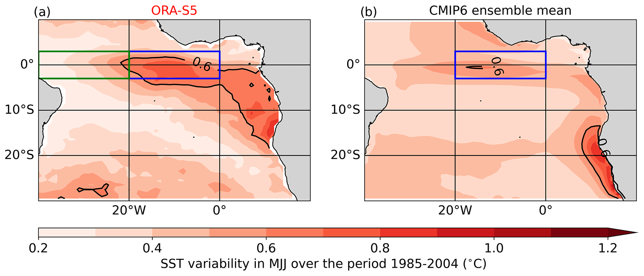
Figure 1 Interannual SST variability in the tropical Atlantic during MJJ. Standard deviation of the MJJ-averaged SST anomalies for (a) ORA-S5 and (b) CMIP6 ensemble mean, spanning from January 1985 to December 2004. The CMIP6 ensemble is composed of 55 models listed in Table S1 in the Supplement. The blue and green boxes represent the ATL3 (3° S–3° N, 20° W–0° E) and ATL4 (3° S–3° N, 40–20° W) regions, respectively.

Despite substantial warm biases having been found in state-of-the-art coupled general circulation models (CGCMs) in the EEA (Davey et al., 2002; Richter and Tokinaga, 2020; Farneti et al., 2022), CGCMs are still capable of reproducing the BF (Deppenmeier et al., 2016). A number of them manage to simulate realistic interannual SST variability within the ATL3 during boreal summer (Fig. 1b; see also Richter and Tokinaga, 2020). However, while the CGCM ensemble mean depicts too-weak interannual SST variability in the EEA, it shows excessive interannual SST variability off the coasts of Angola and Namibia during boreal summer (Fig. 1b). Prodhomme et al. (2019) showed, using Coupled Model Intercomparison Project (CMIP) Phase 5 simulations, that the representation of the Atlantic Niño is strongly linked to the cold-tongue development, highlighting the importance of accurately capturing the seasonal evolution of the wind stress and SST in CGCMs. CGCMs have been extensively evaluated in the tropical Atlantic region, serving as valuable tools for comprehending and predicting variability patterns (Crespo et al., 2022; Prigent et al., 2023a, b). To our knowledge, relatively little effort has been devoted to the simulation of interannual variability in ocean general circulation models (OGCMs) in the tropical Atlantic. Wen et al. (2017) analyzed the response of tropical ocean simulations with two different surfaces forcings: the National Centers for Environmental Prediction/DOE Reanalysis 2 (NCEP/DOE-R2; Kanamitsu et al., 2002) and the Climate Forecast System Reanalysis (CFSR; Saha et al., 2010). They found that the magnitude of the ocean temperature variability simulated using these two surface forcings was comparable in the tropical Pacific; however, they showed that using CFSR led to some improvements in the tropical Atlantic, emphasizing that the improvements in the tropical Atlantic were mainly attributable to differences in surface winds.

The Ocean Model Intercomparison Project (OMIP; Griffies et al., 2016) provides an ideal framework for evaluating the simulation of the interannual variability in the equatorial Atlantic by ocean models. The main objective of OMIP is to provide a framework for assessing, understanding, and improving the ocean and sea-ice components of global climate models that contribute to the CMIP. OMIP has used two atmospheric and river runoff datasets to force ocean sea-ice models. In OMIP Phase 1 (OMIP1; Griffies et al., 2009), the Coordinated Ocean-ice Reference Experiments phase-II atmospheric state (CORE-II; Large and Yeager, 2009), mainly derived from the NCEP atmospheric reanalysis phase 1, was employed. In OMIP Phase 2 (OMIP2; Griffies et al., 2016; Tsujino et al., 2020), the JRA-55-based surface dataset for driving ocean–sea-ice models (JRA55-do; Tsujino et al., 2018) was used. In the present study, we will address the following questions: how well do the OMIP1 and OMIP2 ensembles simulate the monthly climatologies of equatorial Atlantic zonal winds, sea level anomalies (SLAs), and SSTs? What are the differences in the interannual variability within the EEA between OMIP1 and OMIP2? Which component of the atmospheric forcing is responsible for these differences?

To address these questions, we utilize various observational datasets and reanalysis products and conduct sensitivity experiments, all of which are detailed in Sect. 2. We scrutinize the seasonal patterns of equatorial Atlantic zonal winds, SLAs, and SSTs in Sect. 3. Section 4 is dedicated to assessing the interannual SST, sea surface height (SSH), and temperature variability within the OMIP1 and OMIP2 ensembles. In Sect. 5, we delve into the impact of wind forcing on the EEA interannual variability. Final conclusions, along with a discussion, can be found in Sect. 6.

2 Data and methods

2.1 Data

2.1.1 Reanalysis products and observational datasets

This study employs several reanalysis products, all with a monthly temporal resolution if not stated otherwise. Specifically, SST, sea surface height (SSH), zonal wind stress, and upper 200 m depth ocean potential temperature are taken from the Ocean Reanalysis System version 5 (ORA-S5; Zuo et al., 2019). ORA-S5 provides data at a horizontal resolution of 0.25°×0.25° and spans the period from January 1958 to the present day. ORA-S5 has 72 z levels in the ocean. The Optimum Interpolation SST version 2 (OI-SST, Reynolds et al., 2002) is also used; it is available at a horizontal resolution of 1°×1° over the period from December 1981 to January 2023. Additionally, zonal winds at 10 m height (U10) are obtained from the CORE-II atmospheric state (Large and Yeager, 2009), with a horizontal resolution of 2°×2° and a temporal resolution of 6 h, encompassing the period from January 1948 to December 2009, and from the JRA55-do atmospheric forcing derived from the Japanese 55-year Reanalysis (Griffies et al., 2016; Tsujino et al., 2018), with a horizontal resolution of 0.5625° × 0.5625° (∼ 55 km × 55 km at the Equator) and a temporal resolution of 3 h, spanning from January 1958 to December 2018. In addition to reanalysis products, zonal winds at 10 m height are taken from the Cross-Calibrated Multi-Platform version 2 (CCMP v2; Mears et al., 2019), providing data at a horizontal resolution of 0.25° × 0.25° and spanning from January 1988 to December 2017. To validate the SLA from the OMIP models, we compare it to the monthly mean gridded AVISO data (version vDT2021) distributed by the Copernicus Climate Change Service (C3S, 2018) and available at a horizontal resolution of 0.25° × 0.25°, spanning the period from January 1993 to present.

2.1.2 OMIP data

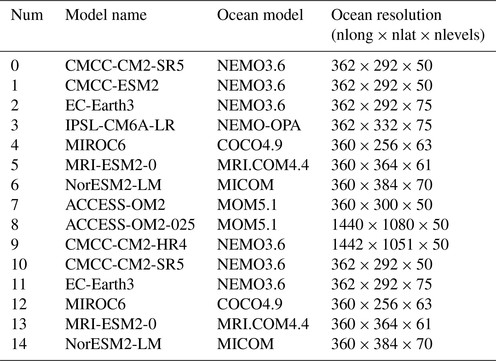
In this study, we assess how models participating in OMIP1 and OMIP2 simulate the equatorial Atlantic interannual variability. The OMIP1 protocol consists of five consecutive cycles of the 62-year-long CORE-II atmospheric state (Large and Yeager, 2009), whereas the OMIP2 protocol consists of six consecutive cycles of the 61-year-long JRA55-do forcing. The JRA55-do has a higher temporal resolution (3 hourly) and a finer spatial resolution (0.5625° × 0.5625°; ∼ 55 km × 55 km at the Equator) than the CORE-II forcing (6 hourly and 2° × 2°). Models participating in both OMIPs have used the same ocean model physics. For the purpose of analysis, we focused on the fifth and sixth cycles of OMIP1 and OMIP2, respectively, during a common period from January 1985 to December 2004, aligning with Farneti et al. (2022). All ocean models with a resolution finer than 1° × 1° and with all the variables needed for this study are listed in Table 1. The considered models were bi-linearly interpolated horizontally onto a regular 1° × 1° grid and vertically at the following depth levels: 6, 15, 25, 35, 45, 55, 65, 75, 85, 95, 105, 115, 125, 135, 145, 156.9, 178.4, 222.5, and 303.1 m. The following variables were utilized in the analysis: SST (variable name: TOS), SSH (variable name: ZOS), zonal wind stress (variable name: UAS), ocean temperature (variable name: THETAO), mixed-layer depth (variable name: MLOTST), and net surface heat flux (variable name: HFDS).

Table 1 OMIP1 models (0–6) and OMIP2 models (7–14) used in this study. The table indicates the model name; the ocean model used; and the number of grid points in the longitudinal, latitudinal, and vertical dimensions.

2.1.3 CMIP6 data

All 55 CMIP6 models from the variant r1i1p1f1 considered in Fig. 1 are listed in Table S1 in the Supplement. We use monthly mean outputs of SST (variable name: TOS) retrieved over the historical period from January 1985 to December 2004. Before analysis, CMIP6 models' outputs were bi-linearly interpolated on a common 1° × 1° regular grid.

2.1.4 Simulations with the GFDL-MOM5 model

We conducted several modeling experiments to complement the OMIP analyses. We employed the NOAA-GFDL Modular Ocean Model version 5 (MOM5; Griffies, 2012), which is a free-surface primitive-equation model and uses a z^* rescaled geopotential coordinate.

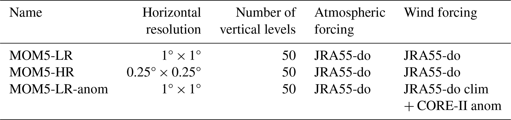
First, we performed a control run (MOM5-LR) following the OMIP2 protocol (Griffies et al., 2016), running the MOM5 ocean model for six consecutive cycles of the 61-year-long JRA55-do forcing. The simulation was conducted at 1° resolution in the horizontal and with 50 vertical levels. In MOM5-LR, subgrid mesoscale processes are parameterized with the Gent–McWilliams skew-flux closure scheme (Gent and Mcwilliams, 1990; Gent et al., 1995; Griffies, 1998) and submesoscale eddy fluxes according to Fox-Kemper et al. (2008) and Fox-Kemper et al. (2011). Vertical mixing is represented with a K-profile parameterization (Large et al., 1994).

Next, we examined the influence of the wind forcing on the EEA interannual variability. An additional experiment, MOM5-LR-anom, mirrors the MOM5-LR configuration, with the exception that we repeated the sixth cycle by replacing the JRA55-do winds at 10 m height (U10 and V10) with a reconstructed wind field. The wind field used in MOM5-LR-anom is the sum of the JRA55-do monthly climatological mean plus the monthly anomalies from the climatological CORE-II winds. As turbulent fluxes of momentum, heat and moisture are derived through bulk formulae based on the near-surface atmospheric state (including 10 m winds); all surface fluxes are expected to be affected by the reconstructed wind field. Also, although not energetically consistent with the other forcing variables, this configuration provides a sensitivity for the upper-ocean response to the wind variability in the CORE-II forcing.

Finally, to assess the impact of the horizontal resolution on the simulation of interannual variability in the EEA, we conducted a MOM5-HR experiment following the OMIP2 protocol. MOM5-HR has a similar configuration to MOM5-LR, but its horizontal resolution is refined to 0.25° × 0.25°, and the parameterization for mesoscale eddy fluxes is turned off. As for OMIP2 and MOM5-LR, we analyzed the sixth cycle of MOM5-HR. In Sect. S1 in the Supplement, we evaluate the outputs of MOM5-LR and MOM5-HR simulations against ORA-S5, focusing on the equatorial Atlantic Ocean mean state, monthly climatology, and interannual temperature variability. This comparison shows that, even though MOM5-LR and MOM5-HR feature some biases, both simulations are able to capture reasonably well the tropical Atlantic mean state, monthly climatology, and upper 200 m temperature variability. MOM5 experiments and their main characteristics are summarized in Table 2.

Table 2 Table summarizing the different configurations of the MOM5 experiments. The table indicates the experiment name, the horizontal resolution, the number of vertical levels, the atmospheric forcing, and the wind forcing. In MOM5-LR-anom, the wind forcing is a synthetic reconstruction obtained from the JRA55-do monthly climatological mean and the CORE-II monthly anomalies based on their climatology.

2.2 Methodology

2.2.1 Definition of anomalies

We compare the EEA interannual variability simulated by the OMIP1 ensemble mean to that simulated by the OMIP2 ensemble mean over a 20-year period spanning from January 1985 to December 2004. Throughout this paper, prior to all analyses, the linear trend is removed pointwise in relation to each dataset. Monthly mean anomalies are computed by subtracting the climatological monthly mean seasonal cycle derived over the study period. The boreal-summer interannual variability is quantified as the standard deviation of the MJJ-averaged anomalies.

2.2.2 Definitions of thermocline depth, mixed-layer depth, and sea level anomaly

The mean depth of the thermocline is defined as the depth of the maximum vertical temperature gradient (dT $/$ dz). SSH anomalies are used as a proxy for thermocline-depth variations. Mixed-layer depth (MLD) is determined as the ocean depth at which the potential density σ_θ has increased by 0.03 kg m⁻³ relative to the top model level value (Griffies et al., 2016). A discussion on the method and its implications in defining MLD in OMIP models can be found in Treguier et al. (2023). The MLD, dT $/$ dz, and the corresponding depth of the maximum dT $/$ dz are shown for each OMIP model and sensitivity experiment in Fig. S1 in the Supplement. Sea level anomaly (SLA) is defined as the pointwise difference between the SSH and the mean sea surface, with the mean sea surface calculated as the SSH average of the period January 1985 to December 2004. The equatorial Atlantic thermocline tilt is defined as the difference in terms of the depth of the maximum dT $/$ dz between the ATL4 and ATL3 regions.

2.2.3 Bjerknes feedback and thermal damping

The three components of the Bjerknes feedback (BF) are assessed as follows. The first component (BF1) is the linear regression of ATL4-averaged zonal wind stress anomalies in MJJ based on ATL3-averaged SST anomalies in MJJ. The second component (BF2) is the linear regression of ATL3-averaged SSH anomalies in MJJ based on ATL4-averaged zonal wind stress anomalies in MJJ. The third component (BF3) is the linear regression of ATL3-averaged SST anomalies in MJJ based on ATL3-averaged SSH anomalies in MJJ. Additionally, the thermal damping is quantified as the linear regression of ATL3-averaged net heat flux anomalies in MJJ based on ATL3-averaged SST anomalies in MJJ.

3 Comparison of the OMIP1 and OMIP2 equatorial Atlantic monthly climatologies

Accurately simulating the equatorial Atlantic wind, SLA, and SST monthly climatologies in ocean models is crucial for the good representation of the EEA interannual SST variability (Prodhomme et al., 2019). Therefore, in this section, we compare the OMIP1 and OMIP2 monthly climatological means of the equatorial Atlantic (3° S–3° S, 40° W–10° E) zonal winds, SLAs, and SSTs to reanalysis products and observational datasets. A comparison to the Prediction and Research Moored Array in the Tropical Atlantic (PIRATA; Servain et al., 1998; Bourlès et al., 2008) at the equatorial moorings of 35° W, 23° W, 10° W, and 0° E can be found in Text S2.

The monthly climatology of the zonal wind in the western equatorial Atlantic is dominated by an annual cycle with maximum easterly winds in September–October–November (SON) and minimum easterlies in MAM (Fig. 2a). Meanwhile, the EEA zonal wind exhibits a semiannual cycle (Fig. 2a), with maxima in January–February–March and SON. Both CORE-II (Fig. 2b) and JRA55-do (Fig. 2c) surface forcings closely mirror the observed monthly climatology of the zonal wind in the equatorial Atlantic. In the ATL4 region (Fig. 2d), CORE-II and JRA55-do zonal winds are stronger than those of CCMP v2 throughout the year.

Next, we analyze the seasonal cycle of the SLA, where negative (positive) SLA indicates a shoaling (deepening) of the thermocline. Consistently with the strong link between western equatorial Atlantic zonal winds and the thermocline (Philander and Pacanowski, 1986), the seasonal cycle of the SLA depicts an annual cycle in the west (Fig. 2e). In the east, a semiannual cycle appears in the SLA. Brandt et al. (2016) showed that the equatorial Atlantic seasonal cycle of SLA is driven by resonance modes associated with the second and fourth baroclinic modes at semiannual and annual frequencies, respectively. In the western equatorial Atlantic, the thermocline reaches its shallowest point during MAM, and this signal progresses eastward, reaching 10° W by July. In SON, the thermocline is deep in the west, and the signal also propagates eastward, but its propagation is faster. These eastward-propagating SLA signals can be understood in terms of linear dynamics and are essentially explained by the first four baroclinic modes (Ding et al., 2009). Both the OMIP1 (Fig. 2f) and OMIP2 (Fig. 2g) ensemble means exhibit patterns that are similar to ORA-S5. In comparison to ORA-S5, the amplitude of the annual cycle in the western equatorial Atlantic is too weak in both OMIP ensembles (Table 3). However, relative to the OMIP2 ensemble mean, the annual cycle of the SLA in the western equatorial Atlantic is 40 % larger in the OMIP1 ensemble mean. In the ATL3 region (Fig. 2h), the shoaling of the thermocline in JJA, as indicated by the negative SLA, is about 30 % too weak in both OMIP ensembles in comparison to ORA-S5 (Table 3).

The shoaling of the thermocline depth from MAM to JAS in the ATL3 region (Fig. 2h) is closely related to the rapid decrease in SST (Fig. 2i). In ORA-S5, the ATL3-averaged SST decreases from 28.52 °C in MAM to 24.79 °C in JAS, with a cooling of 3.73 °C (Table 3). In comparison to ORA-S5, both OMIP ensemble means (Fig. 2j, k) generate a weaker cooling in the ATL3 region (3.19 ± 0.1 °C for OMIP1 and 3.29 ± 0.15 °C for OMIP2, Fig. 2l) from MAM to JAS. It is noteworthy that the difference in cooling between the OMIP1 and OMIP2 ensemble means is mainly due to slightly warmer ATL3 SSTs in MAM for OMIP2 compared to for OMIP1.

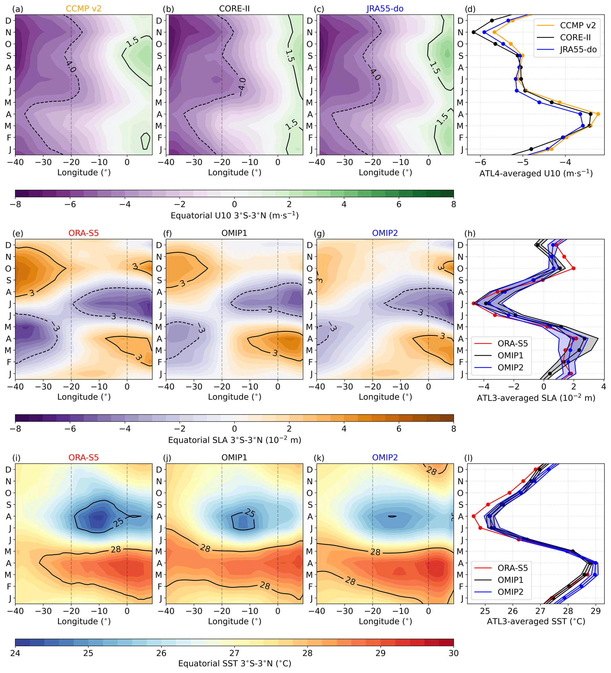
Figure 2 Hovmöller diagrams of monthly climatologies for equatorial Atlantic U10, SLA, and SST. (a) Monthly climatology of CCMP v2 U10, averaged between 3° S and 3° N and presented as a function of longitude and calendar month for the period January 1988 to December 2004. (b, c) Same as (a) but for CORE-II and JRA55-do U10 over the period January 1985 to December 2004. (d) Monthly climatologies of the ATL4-averaged U10 from CCMP v2 (orange), CORE-II (black), and JRA55-do (blue). (e, f, g) Monthly climatologies of SLA in ORA-S5, OMIP1 ensemble mean, and OMIP2 ensemble mean, averaged between 3° S and 3° N, shown as a function of the longitude and calendar month for the period from January 1985 to December 2004. (h) Monthly climatologies of the ATL3-averaged SLA from ORA-S5 (red), OMIP1 (black), and OMIP2 (blue). (i, j, k, l) Same as (e, f, g, h) but for the SST.

Table 3 Table summarizing key values allowing for the comparison of OMIP1 and OMIP2 ensemble means to ORA-S5 in the equatorial Atlantic over the period from January 1985 to December 2004. Values in parentheses are for JAS.

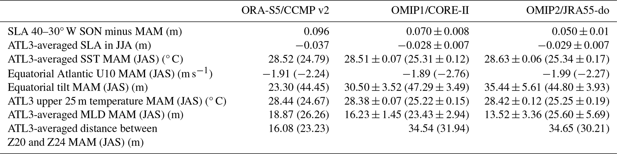
As the monthly climatology of the equatorial Atlantic SST is strongly influenced by subsurface conditions, we examined the upper 200 m ocean temperature during both MAM and JAS (Fig. 3). During MAM (Fig. 3a), the equatorial Atlantic easterly winds (3° S–3° N, 40° W–10° E) are relatively weak, measuring 1.91 m s⁻¹ in CCMP v2. Consequently, the thermocline exhibits a small tilt of 23.30 m, with the upper 25 m in the ATL3 region having a temperature of 28.44 °C. Notably, the ATL3-averaged MLD is located at 18.87 m. We note that the vertical temperature gradient is pronounced in this region, with the distance between the 20 and 24 °C isotherms measuring 16.08 m. In JAS (Fig. 3b), the equatorial Atlantic easterlies intensify to 2.24 m s⁻¹, leading to a steeper thermocline with a tilt of 44.45 m and an increased slope of the isotherms between 20° W and 0° E. The upper 25 m in the ATL3 experiences a strong cooling, with a temperature of 24.67 °C, while the MLD deepens to 26.26 m.

Comparing the above values to the OMIP ensemble means (Table 3), we observe that the upper 200 m temperature sections in both MAM (Fig. 3c, e) and JAS (Fig. 3d, f) align closely with those of ORA-S5. However, some differences are listed next. In MAM (Fig. 3c, e), the CORE-II (JRA55-do) easterlies in the equatorial Atlantic are slightly weaker (stronger) than CCMP v2, and the tilt of the thermocline is overestimated in both OMIP ensembles. The upper 25 m temperature in the ATL3 region is well captured by the OMIP1 and OMIP2 ensemble means, but, in both ensembles, the MLD is too shallow (Table 3). Relative to ORA-S5, both OMIP ensembles feature a too-diffusive thermocline, as indicated by the large distance between the 20 and 24 °C isotherms in the ATL3 region (Table 3). In JAS (Fig. 3d, f), the equatorial Atlantic easterlies are overestimated in both ensembles; however, the tilt of the thermocline in the OMIP ensembles is close to the one from ORA-S5 (Table 3). The upper 25 m temperature from the OMIP ensemble means in the ATL3 is not cooling as much as in ORA-S5 (Table 3). Finally, the deepening of the ATL3-averaged MLD is better represented in the OMIP2 ensemble than in the OMIP1 ensemble (Table 3).

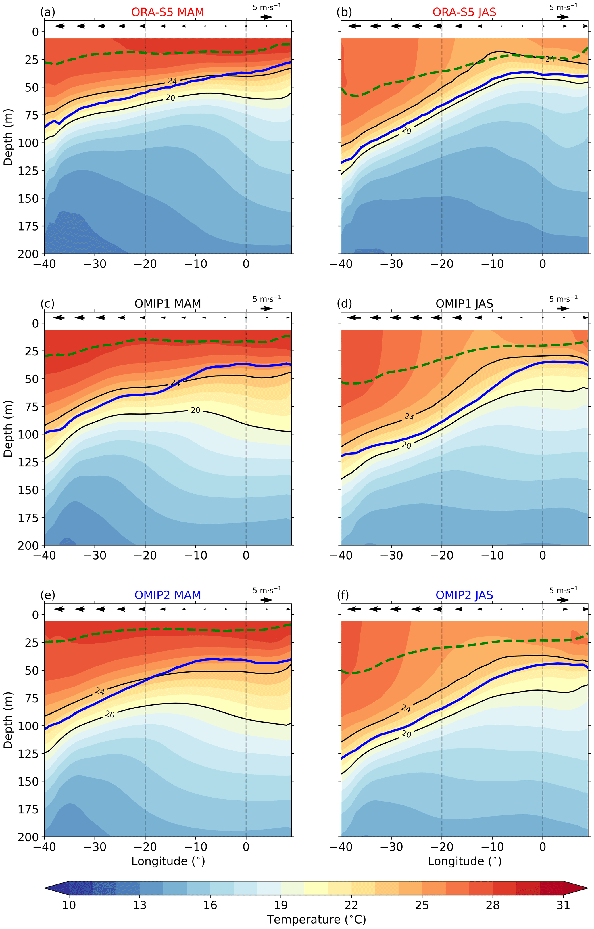
Figure 3 Upper 200 m ocean temperature for MAM (left) and JAS (right). (a, c, e) MAM upper 200 m ocean temperature in the equatorial Atlantic (3° S–3° N, 40° W–9° E), shown by shading, where black arrows indicate zonal wind at 10 m height; thick blue lines denote the maximum dT $/$ dz; dashed green lines represent the mixed-layer depth; and black lines indicate the depths of the 20 and 24 °C isotherms for ORA-S5, OMIP1, and OMIP2 ensemble means. (b, d, f) Same as (a, c, e) but for JAS. Vertical dashed black lines denote the ATL3 region.

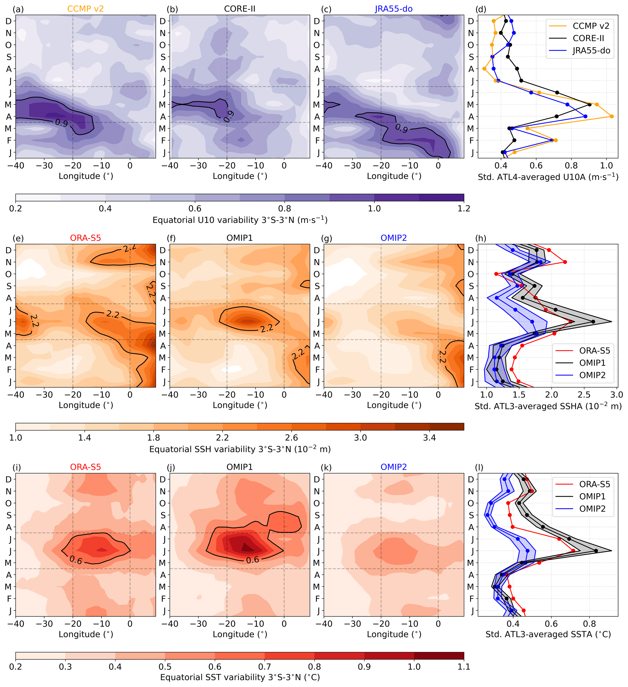
Figure 4 Same as Fig. 2 but for the monthly climatological standard deviation of interannual anomalies. The vertical lines in panels (a), (b), and (c), denote the ATL4-region, whereas in panels (e), (f), (g), (i), (j), and (k) the vertical lines denote the ATL3 region. The horizontal lines in panels (a), (b), and (c) highlight the AMJ months, whereas in panels (e), (f), (g), (i), (j), and (k) the horizontal lines highlight the MJJ months.

To summarize this section and answer the first question raised in the introduction, we find that the OMIP1 and OMIP2 ensemble means closely replicate the monthly climatologies of equatorial Atlantic zonal winds, SSTs, SLAs, and upper 200 m ocean temperatures when compared to ORA-S5 and CCMP v2. Nonetheless, we highlight some discrepancies relative to ORA-S5: (1) the seasonal shoaling of the thermocline in JJA is about 30 % weaker in both OMIP ensemble means, (2) both OMIP ensemble means exhibit a too-diffusive thermocline, and (3) the cooling of the SST and upper 25 m ocean temperature from MAM to JAS in the ATL3 is less pronounced in the OMIP ensemble means.

4 Comparison of OMIP1 and OMIP2 equatorial Atlantic interannual variabilities

The interannual variability in the equatorial Atlantic exhibits a pronounced seasonality (Keenlyside and Latif, 2007; Lübbecke et al., 2018). Specifically, high interannual zonal wind variability in CCMP v2 in the western equatorial Atlantic occurs from 40–20° W during April–May–June (Fig. 4a) and from 20–15° W in March and April. As OMIP1 and OMIP2 models are forced by the CORE-II and JRA55-do 10 m winds, respectively, we compare them to CCMP v2. The CORE-II zonal wind forcing displays a similar pattern to CCMP v2 from 40–20° W but with weaker interannual variability (Fig. 4b). The JRA55-do forcing also exhibits a similar pattern of interannual zonal wind variability but underestimates it in April–May–June (Fig. 4c). Additionally, the JRA55-do forcing (Fig. 4c) reveals high zonal wind variability between 10° W and 10° E in January and February, which is not as prominent in CCMP v2 (Fig. 4a) and is absent in the CORE-II forcing (Fig. 4b). Quantitatively, the standard deviation of AMJ-averaged U10 anomalies in the ATL4 region is 0.80 m s⁻¹ for CCMP v2 over the period from January 1988 to December 2004 and 0.70 and 0.68 m s⁻¹ for CORE-II and JRA55-do, respectively, over the period from January 1985 to December 2004. The ATL4-averaged monthly climatological standard deviation of the U10 anomalies (Fig. 4d) reveals that the peak zonal wind variability is in May for CORE-II and in April for JRA55-do and CCMP v2.

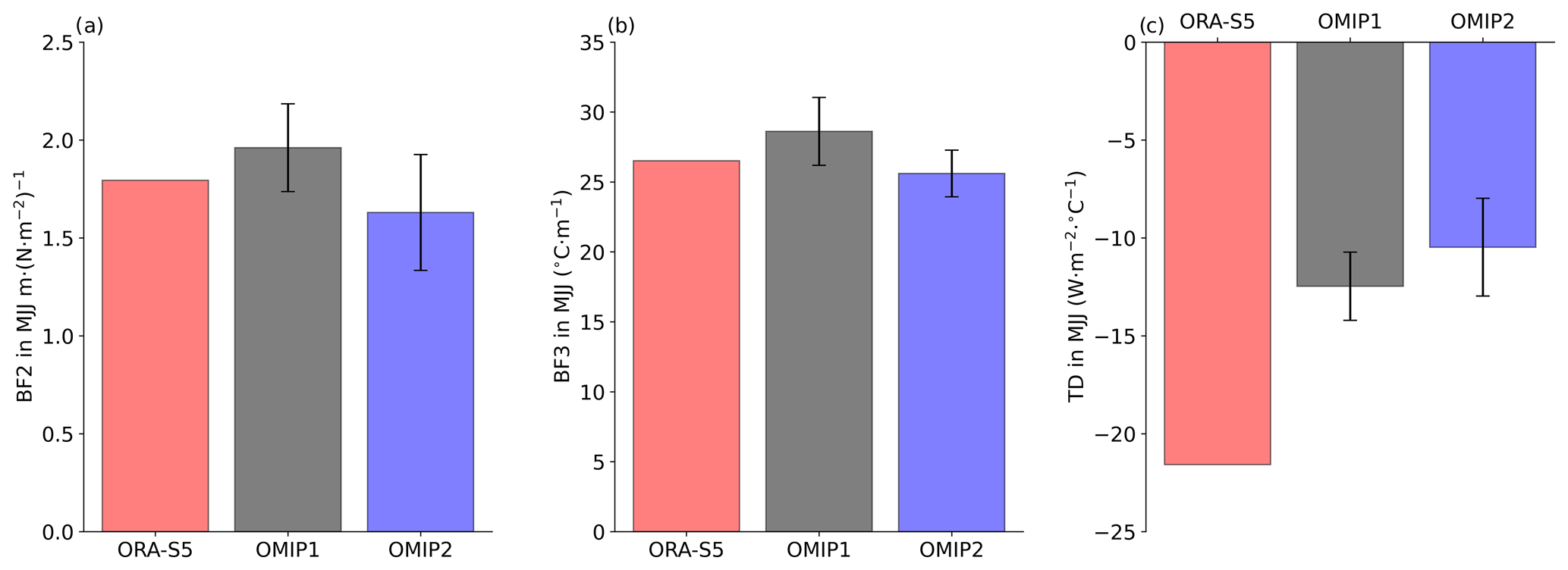
Figure 5 Bjerknes feedback components and thermal damping during MJJ over the period from January 1985 to December 2004. (a) Histogram of the BF2 in MJJ for ORA-S5 (red), the OMIP1 ensemble (gray), and the OMIP2 ensemble (blue). (b) Same as (a) but for the BF3. (c) Same as (a) but for the thermal damping (TD). Error bars are defined as ± 1 standard deviation of the ensemble.

Typically, sudden relaxation (intensification) of the trade winds in the western equatorial Atlantic can trigger interannual downwelling (upwelling) equatorial Kelvin waves (Illig et al., 2004). While propagating eastward along the equatorial wave guide, these waves generate thermocline-depth variations which can be observed in the SSH anomalies. In the following, we compare the equatorial Atlantic interannual SSH variability in the OMIP1 and OMIP2 ensemble means to that of ORA-S5. In ORA-S5, two peaks of interannual SSH variability are observed during boreal summer, one between 40 and 35° W and another between 20° W and 0° E (Fig. 4e). Additionally, ORA-S5 exhibits high interannual SSH variability in November–December in the EEA (Fig. 4e). The interannual SSH variability in the ATL3 region is too strong (weak) in the OMIP1 (OMIP2) ensemble mean compared to that in ORA-S5 (Fig. 4f, g, h). In numbers, the OMIP1 (OMIP2) ensemble mean ATL3-averaged interannual SSH variability in MJJ is 0.02 ± 0.002 m (0.015 ± 0.002 m), while it is 0.019 m in ORA-S5 (Fig. 4h). The anomaly correlation coefficients and root-mean-square errors between the OMIP1 and OMIP2 ensemble means with AVISO SLA, evaluated over the period January 1993 to December 2004, are shown in Fig. S2a–d. These show high correlations (> 0.75; Fig. S2a, b) and low root-mean-square errors (< 0.01 m; Fig. S2c, d) in the EEA for both OMIP ensemble means, indicating a high fidelity of the OMIP ensembles with AVISO. To further illustrate that, we show the time series depicting ATL3-averaged SSH anomalies for AVISO, OMIP1, and OMIP2 ensemble means in Fig. S2e. Despite robust correlations between both OMIP ensembles and AVISO (0.78), evaluated over the period from January 1993 to December 2004, the amplitude of the monthly mean SSH anomalies is larger in OMIP1 compared to in OMIP2. This indicates that thermocline-depth variations are larger in the OMIP1 ensemble mean compared to in the OMIP2 ensemble mean.

Finally, we compare the equatorial Atlantic interannual SST variability from the OMIP1 and OMIP2 ensemble means to ORA-S5. ORA-S5 displays two peaks of interannual SST variability in the ATL3 region, one in MJJ and another in November–December (Fig. 4i). Both OMIP ensemble means exhibit a similar pattern to ORA-S5. However, relative to ORA-S5, the OMIP1 (OMIP2) ensemble mean overestimates (underestimates) the MJJ interannual SST variability in the EEA (Fig. 4j, k). In numbers, the standard deviations of the MJJ-averaged SST anomalies in the ATL3 region are 0.62 ± 0.04, 0.41 ± 0.03, and 0.59 °C for the OMIP1 and OMIP2 ensemble means and ORA-S5, respectively. The equatorial Atlantic interannual SST variability in MJJ is systematically larger in OMIP1 ensemble members than in OMIP2 ensemble members (Fig. S3). The anomaly correlation coefficients and root-mean-square errors between OMIP1 and OMIP2 simulations with OI-SST, evaluated over the period January 1985 to December 2004, are shown in Fig. S4a–d. In comparison to the tropical Atlantic ocean, the EEA and southeastern tropical Atlantic display the lowest anomaly correlation and the greatest root-mean-square errors across both the OMIP1 and OMIP2 ensembles. This indicates that these regions exhibit the most pronounce biases between both the OMIP ensembles and OI-SST. Nevertheless, it is important to highlight that, despite these differences, the anomaly correlation coefficient is high (≈ 0.8; Fig. S4a, b), and the root mean-square error is low (< 0.5 °C; Fig. S4c, d). To elaborate on this point, we present the time series depicting the ATL3-averaged SST anomalies for the OI-SST, OMIP1, and OMIP2 ensemble means in Fig. S4e. Both the OMIP1 and OMIP2 ensemble means are highly correlated to OI-SST, with Pearson correlation coefficients of 0.79 and 0.80, respectively. However, the ATL3-averaged SST anomalies in the OMIP1 ensemble mean are, in general, larger than in the OMIP2 ensemble mean.

Ocean–atmosphere interactions are key drivers of the interannual SST variability within the EEA (Jouanno et al., 2017). To delve into this, we examined the various components of the Bjerknes feedback and thermal damping in ORA-S5, along with the ensemble means of OMIP1 and OMIP2 (Fig. 5), over the period January 1985 to December 2004. The first component of the Bjerknes feedback is not discussed given that, in a forced ocean model simulation, there is no response of the western equatorial Atlantic winds to the SST anomalies in the eastern equatorial Atlantic. In comparison to ORA-S5, for which the BF2 (Fig. 5a) amounts to 1.79 m (N m⁻²)⁻¹, the OMIP1 (OMIP2) ensemble overestimates (underestimates) it, with a slope of 1.96 ± 0.22 m (N m⁻²)⁻¹ (1.63 ± 0.30 m (N m⁻²)⁻¹). Regarding the BF3 (Fig. 5b), it is equal to 26.51 °C m⁻¹ for ORA-S5 and 28.62 ± 2.42 and 25.60 ± 1.67 °C m⁻¹ for the OMIP1 and OMIP2 ensembles, respectively. Hence, the subsurface–surface coupling is more pronounced in the OMIP1 ensemble mean than in the OMIP2 ensemble mean. Lastly, the thermal damping is assessed (Fig. 5c). While ORA-S5 depicts a strong thermal damping (−21.58 W m⁻² °C⁻¹), both OMIP ensembles underestimate it, with slopes of −12.47 ± 1.74 and −10.48 ± 2.5 W m⁻² °C⁻¹ for the OMIP1 and OMIP2 ensembles, respectively.

The contrast between the interannual variability of the equatorial Atlantic in the OMIP1 and OMIP2 ensemble means extends beyond the surface, as illustrated by the upper 200 m temperature variability in MJJ (Fig. 6). In ORA-S5 (Fig. 6a), two maxima of interannual temperature variability are observed in MJJ, one between 40 and 30° W and another between 20° W and 0° E within ± 10 m range around the mean thermocline. The standard deviation of the ORA-S5 equatorial Atlantic SSH anomalies in MJJ mirrors the upper 200 m interannual temperature variability. The high interannual temperature variability in the western equatorial Atlantic is situated at a depth of 90 m, making it too deep to reach the MLD and, hence, affect the SST. In contrast, the maximum temperature variability in the EEA is located at 50 m depth, closer to the MLD, with an average of 1.28 °C for ORA-S5 when considering the ATL3 region and a ± 10 m range around the mean thermocline. The MJJ interannual temperature variability in the equatorial Atlantic for the OMIP ensemble means (Fig. 6b, c) exhibits a similar pattern to ORA-S5 but with a generally weaker interannual temperature variability. For both OMIP ensembles, the MJJ equatorial Atlantic interannual SSH variability mirrors the upper 200 m interannual temperature variability. The standard deviations of the MJJ-averaged temperature anomalies within ± 10 m of the mean thermocline for the ATL3 region are 0.78 ± 0.06 and 0.58 ± 0.07 °C for the OMIP1 and OMIP2 ensembles, respectively. The upper 200 m interannual temperature variability in the EEA during MJJ is systematically larger in OMIP1 ensemble members compared to in OMIP2 ensemble members, as shown in Fig. S5. Given that both OMIP ensemble means exhibit a similar vertical temperature gradient during boreal summer within ± 10 m of the mean thermocline in the ATL3 region, amounting to −0.15 ± 0.001 °C m⁻¹, it can be inferred that the disparities in the equatorial Atlantic interannual temperature variability are primarily driven by larger fluctuations in the thermocline depth. In contrast, the boreal summer vertical temperature gradient for ORA-S5 within ± 10 m of the mean thermocline in the ATL3 region is −0.25 °C m⁻¹, which can account for its substantially higher subsurface temperature variability.

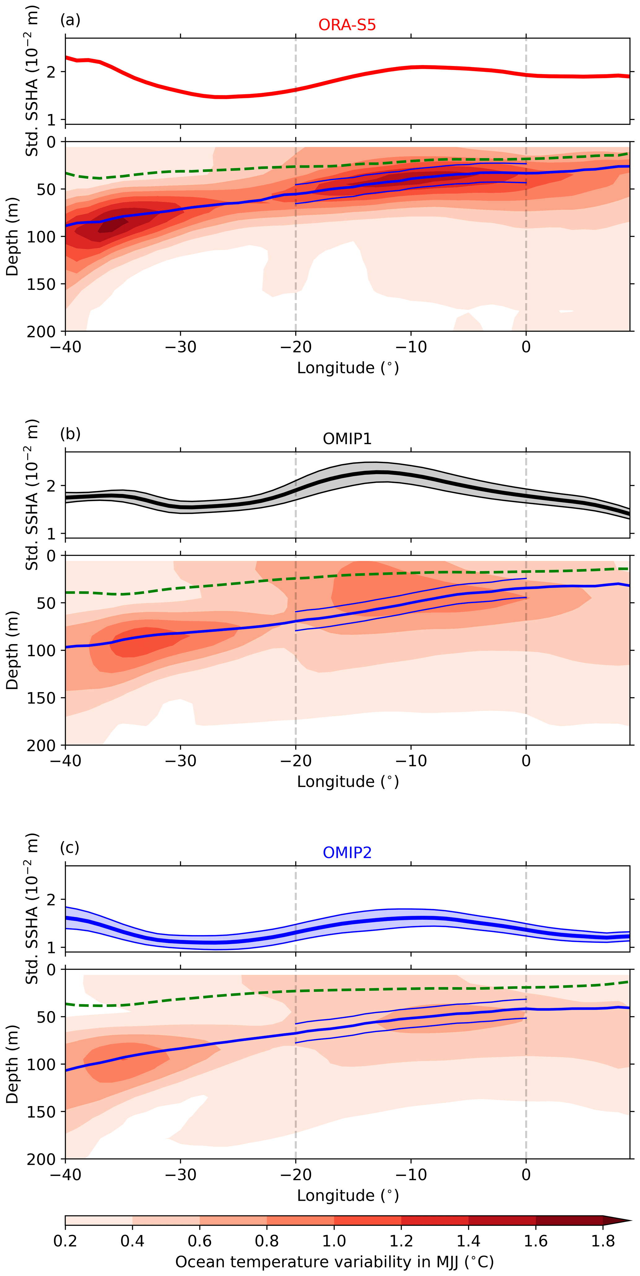
Figure 6 Equatorial Atlantic (3° S–3° N, 40° W–9° E) interannual variability of SSH and upper 200 m ocean temperature during MJJ over the period from January 1985 to December 2004 for (a) ORA-S5, (b) the OMIP1 ensemble mean, and (c) the OMIP2 ensemble mean. Thick blue lines represent the depth of maximum dT $/$ dz, while dashed green lines denote the mixed-layer depth. Thin blue lines encompass a ± 10 m range around the mean thermocline. Vertical dashed lines in black denote the ATL3 region.

In response to the second question raised in the introduction, we showed that, during the period January 1985 to December 2004, the OMIP1 ensemble exhibits about 51 % (34 %) greater boreal summer interannual SST (temperature) variability in the ATL3 region compared to the OMIP2 ensemble. Over the same period and relative to the OMIP2 ensemble, the OMIP1 ensemble has about 33 % greater interannual SSH variability in MJJ in the ATL3 region. When contrasting the two ensembles, the OMIP1 ensemble displays a stronger BF2 and BF3, which could account for the larger interannual SST variability. However, the thermal damping is more prominent in the OMIP1 ensemble than in the OMIP2 ensemble. In the next section, we investigate the impact of the CORE-II and JRA55-do wind forcings on the EEA interannual variability.

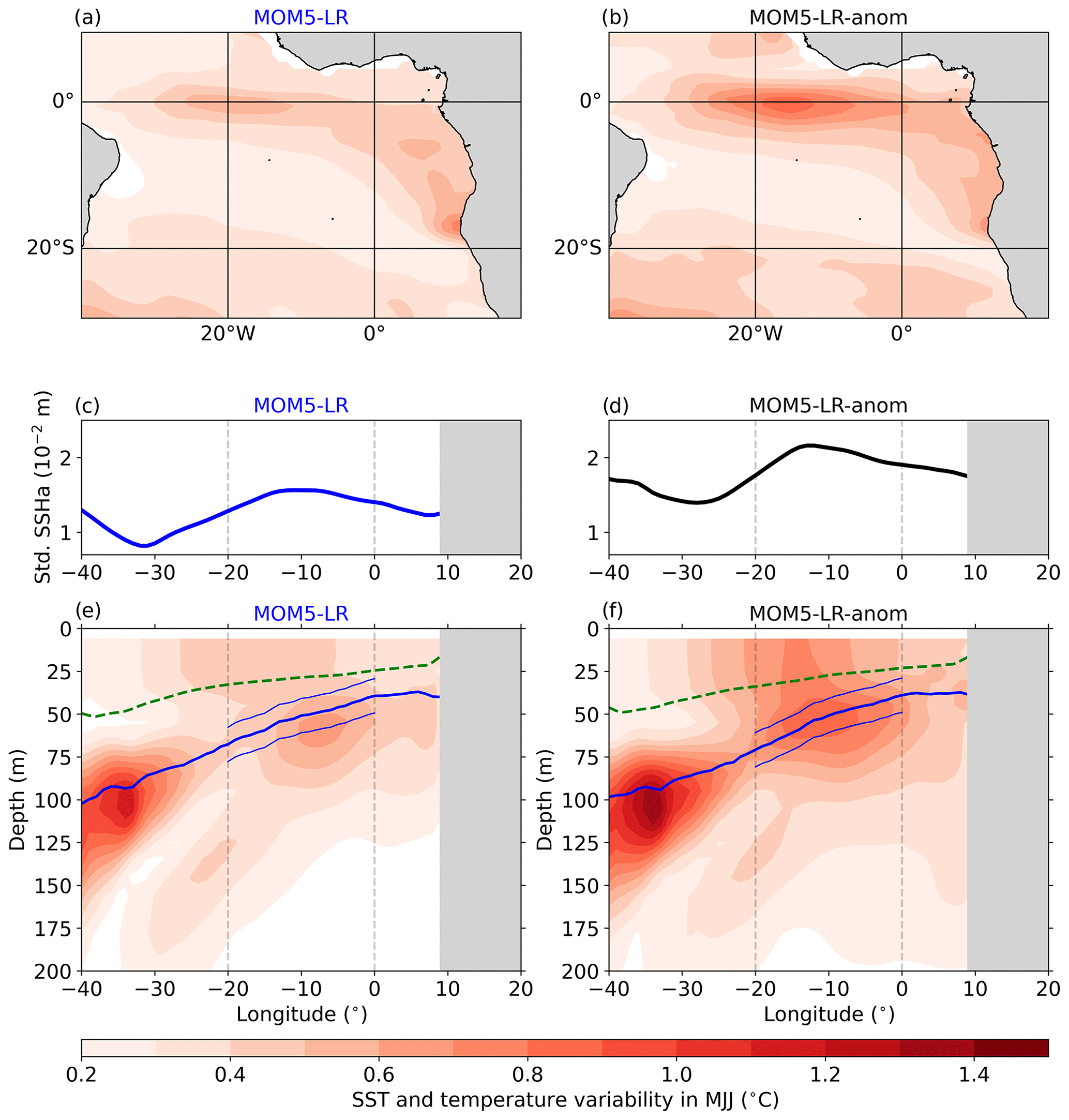
Figure 7 Interannual SST, SSH, and upper 200 m temperature variability during MJJ over the period from January 1985 to December 2004. (a) Standard deviation of SST anomalies averaged over MJJ for MOM5-LR. (c) Standard deviation of SSH anomalies in the equatorial Atlantic (3° S–3° N) during MJJ for MOM5-LR. (e) Standard deviation of the equatorial Atlantic MJJ upper 200 m temperature anomalies for MOM5-LR. (b, d, f) Same as (a, c, e) but for MOM5-LR-anom. The dashed green lines represent the MLD. The solid blue lines indicate the depth of the maximum vertical temperature gradient in MJJ. Thin blue lines encompass a ± 10 m range around the mean thermocline. Vertical dashed black lines denote the ATL3 region.

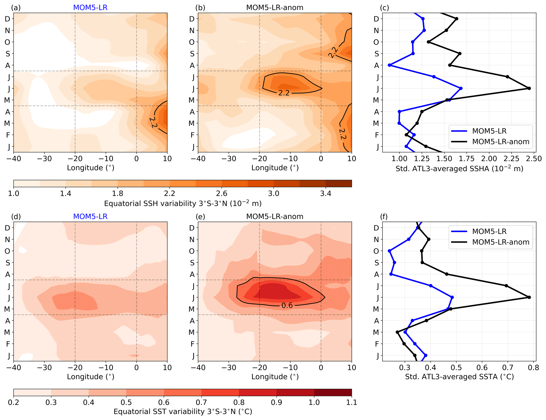
Figure 8 Hovmöller diagrams depicting the interannual variability of SSH and SST over the period from January 1985 to December 2004. (a) Monthly climatological standard deviation of the MOM5-LR sea surface height anomaly (SSHA), averaged between 3° S and 3° N, plotted as a function of longitude and calendar month. (b) Same as (a) but for MOM5-LR-anom. (c) Monthly climatological standard deviation of the ATL3-averaged SSHA for MOM5-LR (blue) and MOM5-LR-anom (black). (d, e, f) Same as (a, b, c) but for the sea surface temperature anomaly (SSTA).

5 Influence of the wind forcing on the equatorial Atlantic interannual variability

Wind forcing is an important driver for the equatorial Atlantic mean state, seasonal cycle, and interannual variability (Richter et al., 2012; Wahl et al., 2011). Wen et al. (2017) investigated the response of tropical ocean simulations to NCEP/DOE-R2 and CFSR surface fluxes, and, using sensitivity experiments with the GFDL MOM version 4p1 (Griffies, 2009), they found that prescribing CFSR surface fluxes instead of NCEP/DOE-R2 surface fluxes significantly improved the simulation of the SST and SSH variabilities in the tropical Atlantic Ocean. In the following, we aim to examine the hypothesis that the different equatorial Atlantic interannual variabilities observed in the OMIP ensemble means are a direct consequence of the discrepancies in wind forcing. A comparison of the CORE-II and JRA55-do reanalyses to other reanalysis products can be found in Text S3. To investigate this, we employ two simulations, namely MOM5-LR and MOM5-LR-anom, as described in Sect. 2.1.4 and compared in Fig. 7.

Both MOM5-LR (Fig. 7a) and MOM5-LR-anom (Fig. 7b) depict high boreal summer interannual SST variability within the ATL3 region. Yet, the MOM5-LR-anom simulation exhibits a larger interannual SST variability, amounting to 0.62 °C, in contrast to 0.42 °C for MOM5-LR. This implies that solely replacing JRA55-do monthly wind anomalies with CORE-II monthly wind anomalies results in a 48 % increase in the EEA interannual SST variability. The equatorial Atlantic SSH variability in boreal summer also depicts an increase in MOM5-LR-anom (Fig. 7d) relative to MOM5-LR (Fig. 7c). Furthermore, this increase is not limited to the surface as it is also reflected in the upper 200 m interannual temperature variability during boreal summer. Specifically, the MJJ interannual temperature variability within a ± 10 m range around the mean thermocline is 0.49 °C for MOM5-LR (Fig. 7e) and 0.74 °C for MOM5-LR-anom (Fig. 7f). Hence, using CORE-II monthly wind anomalies leads to a 51 % increase in boreal summer interannual temperature variability in the ATL3 region and within ± 10 m of the mean thermocline.

The impact of the wind forcing on the equatorial Atlantic interannual variability is further examined in Fig. 8. In comparison to MOM5-LR (Fig. 8a), MOM5-LR-anom (Fig. 8b) exhibits a similar pattern of equatorial Atlantic interannual SSH variability, albeit with a larger magnitude. Quantitatively, the standard deviation of MJJ-averaged SSH anomalies in the ATL3 region amounts to 0.015 m for MOM5-LR and 0.020 m for MOM5-LR-anom. Furthermore, there seems to be a shift of about 1 month in the interannual SSH variability in the EEA when comparing Fig. 8a and b. The monthly climatological standard deviation of the ATL3-averaged SSH anomalies (Fig. 8c) shows that, even though MOM5-LR and MOM5-LR-anom both peak in June, the interannual SSH variability is stronger in May in MOM5-LR than in MOM5-LR-anom, while the opposite is the case in July. This temporal shift of about 1 month in the EEA interannual SSH variability could be related to the different peaks in zonal wind variability in the ATL4 region between JRA55-do (April) and CORE-II (May). As previously discussed, we also find increased interannual SST variability in MOM5-LR-anom (Fig. 8e) relative to MOM5-LR (Fig. 8d). As for the ATL3 interannual SSH variability, a shift of about 1 month is also observed in the interannual SST variability when comparing MOM5-LR to MOM5-LR-anom (Fig. 8f).

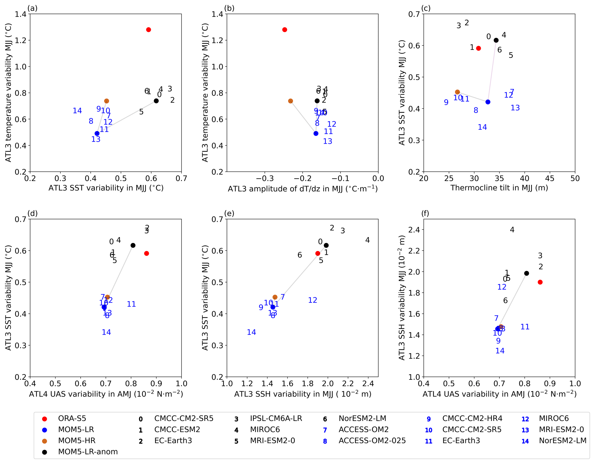
Figure 9 Scatterplots illustrating various equatorial Atlantic metrics assessed during the period January 1985 to December 2004. (a) Relationship between the standard deviation of ATL3-averaged SST anomalies in MJJ and the ATL3-averaged temperature anomalies in MJJ within ± 10 m around the mean thermocline. (b) Relationship between ATL3-averaged dT $/$ dz within ± 10 m around the mean thermocline in MJJ and the ATL3-averaged temperature anomalies in MJJ within ± 10 m around the mean thermocline. (c) Relationship between the equatorial Atlantic thermocline tilt in MJJ and the standard deviation of ATL3-averaged SST anomalies in MJJ. The equatorial thermocline tilt is defined as the difference between the ATL4-averaged and ATL3-averaged depth of the maximum dT $/$ dz. (d) Relationship between the standard deviation of ATL4-averaged UAS anomalies in AMJ and the standard deviation of ATL3-averaged SST anomalies in MJJ. (e) Relationship between the standard deviation of ATL3-averaged SSH anomalies in MJJ and the standard deviation of ATL3-averaged SST anomalies in MJJ. (f) Relationship between the standard deviation of ATL4-averaged UAS anomalies in MJJ and the standard deviation of ATL3-averaged SSH anomalies in MJJ. Dots are color-coded: red, blue, brown, and black dots represent ORA-S5, MOM5-LR, MOM5-HR, and MOM5-LR-anom, respectively. Black (blue) numbers denote the OMIP1 (OMIP2) models.

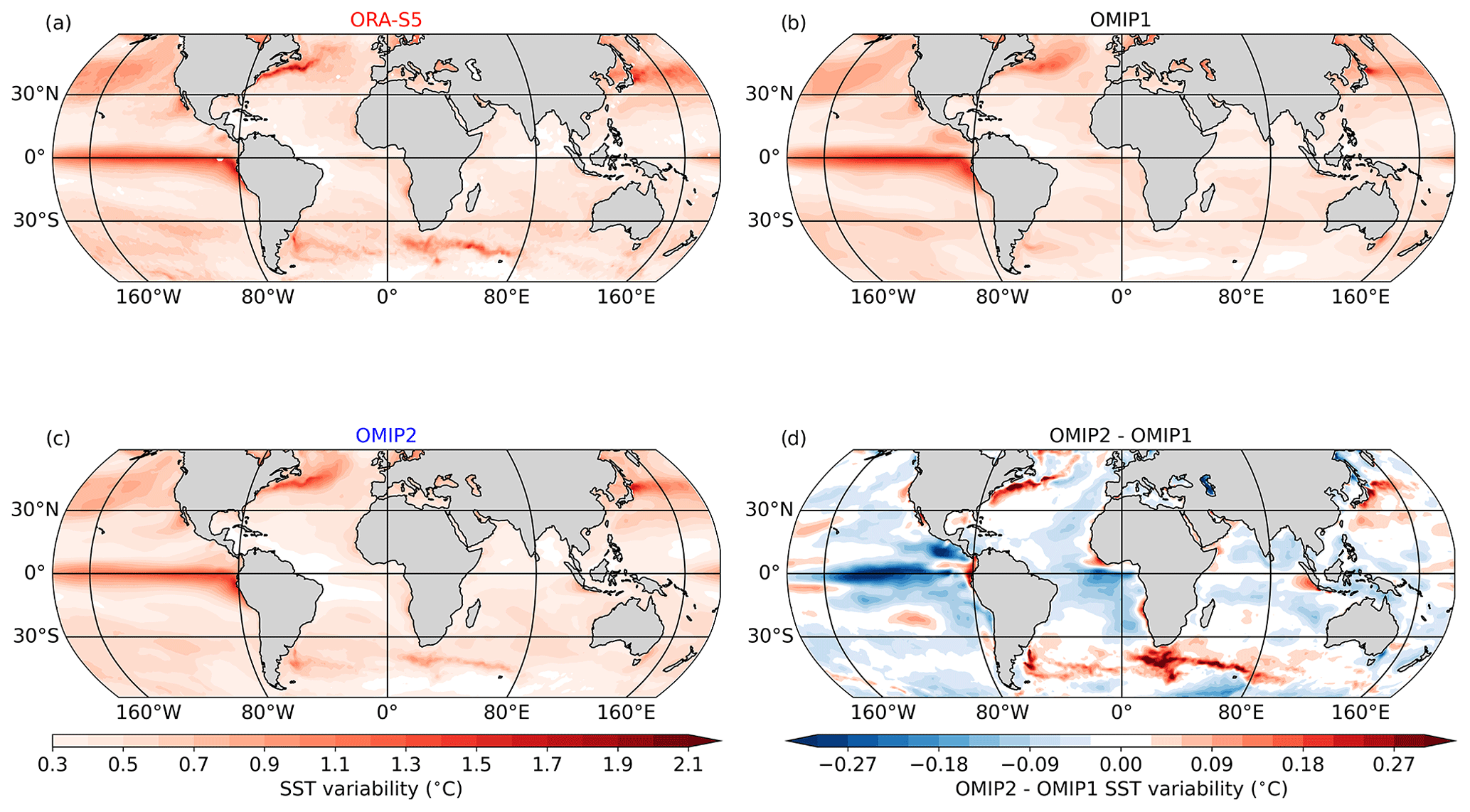
Figure 10 Standard deviation of monthly mean SST anomalies for (a) ORA-S5, (b) the OMIP1 ensemble mean, and (c) the OMIP2 ensemble mean spanning from January 1985 to December 2004. (d) Difference between the OMIP2 ensemble mean minus the OMIP1 ensemble mean.

This section allowed us to answer the last question raised in the introduction. Namely, we have shown that the surface forcing and, in particular, the wind variability have a significant impact on the equatorial Atlantic interannual variability. Indeed, replacing the JRA55-do monthly wind anomalies with the CORE-II monthly wind anomalies results in a substantial increase in ATL3 interannual SST (48 %), SSH (33 %), and temperature (51 %) variability during MJJ, rising from 0.42 °C, 0.015 m, and 0.49 °C for MOM5-LR to 0.62 °C, 0.020 m, and 0.74 °C for MOM5-LR-anom.

6 Conclusions and discussions

6.1 Conclusions

In this study, we have compared the monthly climatologies of equatorial Atlantic zonal wind, SLA, and SST from the OMIP1 and OMIP2 ensemble means to those from ORA-S5. Furthermore, we examined the equatorial Atlantic interannual variability within the OMIP models. Finally, we delved into the causes behind the distinct equatorial Atlantic interannual variabilities during boreal summer in the OMIP1 and OMIP2 ensembles using sensitivity experiments. We have shown the following for the period from January 1985 to December 2004:

• The climatological patterns of the equatorial Atlantic zonal wind, SLA, SST, and ocean temperature in the OMIP1 and OMIP2 ensemble means resemble those in ORA-S5. However, some discrepancies are evident. Specifically, the annual cycle of the SLA in the western equatorial Atlantic is too weak in both the OMIP ensemble means, but the OMIP1 ensemble mean annual cycle of the SLA in the western equatorial Atlantic is about 40 % larger than the one of the OMIP2 ensemble mean; the seasonal shoaling of the thermocline in the ATL3 region during JJA is about 30 % too weak in the OMIP ensembles in comparison to ORA-S5; both OMIP ensembles have a too-diffusive thermocline; and the seasonal cooling in SST from MAM to JAS is insufficient in both OMIP ensembles (Fig. 2).

• In the ATL3 region during boreal summer, the OMIP1 ensemble mean depicts a 51 % greater interannual SST variability and a 34 % larger interannual temperature variability at the thermocline level compared to the OMIP2 ensemble mean (Fig. 9a).

• In boreal summer, both OMIP ensembles exhibit a comparable magnitude of dT $/$ dz in the ATL3 region (Fig. 9b). This suggests that, relative to the OMIP2 ensemble, heightened interannual SST and temperature variability in the OMIP1 ensemble cannot be attributed to differences in the magnitude of dT $/$ dz.

• In boreal summer, the equatorial Atlantic thermocline tilt within OMIP models varies between 24 and 39 m, while it reaches 30 m in the case of ORA-S5 (Fig. 9c). No correlation between the thermocline tilt and the ATL3 interannual SST variability is observed in OMIP models. It is worth noting that both MOM5-LR and MOM5-LR-anom exhibit a similar thermocline tilt, suggesting that the increased ATL3 interannual SST variability in MOM5-LR-anom is not attributable to a change in the thermocline tilt (Fig. 9c).

• During AMJ, the zonal wind stress variability in the western equatorial Atlantic is slightly more pronounced in the OMIP1 ensemble mean compared to in the OMIP2 ensemble mean. This difference may have played a role in the heightened interannual SST variability observed in ATL3 within the OMIP1 ensemble mean (as illustrated in Fig. 9d). It is important to stress that the peak in ATL4 zonal wind variability occurs in April for the JRA55-do forcing and in May for the CORE-II forcing.

• Replacing the JRA55-do monthly wind anomalies with the CORE-II monthly wind anomalies results in a 48 % increase in ATL3 boreal-summer interannual SST variability and a 51 % increase in interannual temperature variability at the thermocline level, as depicted in Fig. 9a. This underscores the critical role of interannual anomalies in the wind forcing in accurately simulating the equatorial Atlantic interannual variability within ocean models. It is worth noting that, in comparison to MOM5-LR, the magnitude of dT $/$ dz in MOM5-LR-anom remains unchanged (Fig. 9b).

• In boreal summer, the interannual SSH variability in the ATL3 region is about 33 % greater in the OMIP1 ensemble mean compared to in the OMIP2 ensemble mean (Fig. 9e). Sensitivity experiments reveal that this change in ATL3 interannual SSH variability from the OMIP1 to the OMIP2 ensemble is mainly attributable to wind anomalies from the CORE-II forcing. Indeed, when comparing MOM5-LR to MOM5-LR-anom, the interannual SSH variability in the ATL3 region during boreal summer is heightened by 33 %, as depicted in Figs. 8 and 9f.

In summary, this study has shown, by comparing the OMIP1 and OMIP2 ensembles and by using sensitivity experiments, that seemingly minor uncertainties in the atmospheric forcing can lead to notable discrepancies in the simulated equatorial Atlantic interannual variability. For the equatorial Atlantic, we have shown that the interannual variability in ocean models is particularly sensitive to the wind forcing, in line with results from Wen et al. (2017).

6.2 Discussion

It could be argued that changes in ocean model physics from OMIP1 to OMIP2 could also have led to discrepancies in the simulation of the interannual variability in the equatorial Atlantic. However, models participating in both OMIPs have used the same ocean model physics. Hence, discrepancies in the interannual variability in the EEA should be rooted in the atmospheric forcing. The simulation of the EEA interannual variability by ocean models may be influenced by several factors other than the wind forcing. Beyond the zonal and meridional winds, the forcing from CORE-II and JRA55-do includes shortwave and longwave heat fluxes, precipitation, river runoff, air temperature at 2 m, and evaporation. However, their relative impact on the equatorial Atlantic interannual variability has not been investigated in this study and would require further model experiments and analysis.

Another factor potentially impacting on the simulation of the EEA is the ocean horizontal resolution. Model pairs such as ACCESS-OM2 and ACCESS-OM2-025, MOM5-LR and MOM5-HR, and CMCC-CM2-HR4 and CMCC-CM2-SR5 were compared to each other. Each model pair has the same number of vertical levels, but they differ in their horizontal resolution, going from coarse (1° × 1°) to refined (0.25° × 0.25°). This comparison, based only on three model pairs, suggests that increasing the ocean horizontal resolution does not lead to consistent changes in the equatorial Atlantic mean state and interannual SST variability in boreal summer (Fig. 9). One notable change is the increase in the vertical ocean temperature gradient and subsurface temperature variability in boreal summer when comparing MOM5-LR to MOM5-HR (Fig. 9b). However, this change is not observed in the other two model pairs. A larger number of model pairs would be required to properly assess the impact of horizontal resolution and, ideally, also of vertical resolution on stratification biases. Finally, we note that both the OMIP1 and OMIP2 ensembles are largely biased towards Eulerian vertical coordinate models, whereas a larger representation of models making use of Lagrangian vertical coordinates or generalized vertical coordinates using the vertical Lagrangian-remap method (Griffies et al., 2020), such as MOM6 (Adcroft et al., 2019) and HYCOM (Bleck, 2002), could be extremely beneficial to the ocean-modeling community.

To conclude, our study has underscored the importance of the wind forcing in modeling the interannual variability of the equatorial Atlantic. As a consequence, it is imperative to sustain and enhance wind observations in the tropical Atlantic in order to improve the quality of the reanalysis products in the region. We note that Taboada et al. (2019) conducted a comparative study of different wind reanalysis products and highlighted the lack of agreement among them in the tropics. Our results suggest that, even though the monthly climatology of the equatorial Atlantic winds is relatively well captured by reanalysis datasets, their interannual variability needs more validation in the tropical Atlantic.

Finally, the use of JRA55-do forcing (Tsujino et al., 2018) within OGCMs seems to improve the simulation of SST variability in eddy-rich regions like the Gulf Stream, Kuroshio, Malvinas, and Agulhas currents, as well as in eastern boundary upwelling systems (Fig. 10), probably also due to its higher temporal and spatial resolution compared to the CORE-II atmospheric state (Large and Yeager, 2009). However, the use of the JRA55-do atmospheric forcing results in a weak SST variability not only in the equatorial Atlantic (Fig. 4) but also in the equatorial Pacific (Fig. 10d). Due to its disproportionate role in the global climate at interannual and longer variabilities, further studies should focus on assessing the equatorial Pacific as represented by OMIP1 and OMIP2 models.