the Creative Commons Attribution 4.0 License.
the Creative Commons Attribution 4.0 License.
 | 25 May 2021
Assessment of the spectral downward irradiance at the surface of the Mediterranean Sea using the radiative Ocean-Atmosphere Spectral Irradiance Model (OASIM)
Stefano Salon
Elena Terzić
Watson W. Gregg
Fabrizio D'Ortenzio
Vincenzo Vellucci
Emanuele Organelli
David Antoine
A multiplatform assessment of the Ocean–Atmosphere Spectral Irradiance Model (OASIM) radiative model focussed on the Mediterranean Sea for the period 2004–2017 is presented. The BOUée pour l'acquiSition d'une Série Optique à Long termE (BOUSSOLE) mooring and biogeochemical Argo (BGC-Argo) float optical sensor observations are combined with model outputs to analyse the spatial and temporal variabilities in the downward planar irradiance at the ocean–atmosphere interface. The correlations between the data and model are always higher than 0.6. With the exception of downward photosynthetic active radiation and the 670 nm channel, correlation values are always higher than 0.8 and, when removing the inter-daily variability, they are higher than 0.9. At the scale of the BOUSSOLE sampling (15 min temporal resolution), the root mean square difference oscillates at approximately 30 %–40 % of the averaged model output and is reduced to approximately 10 % when the variability between days is filtered out. Both BOUSSOLE and BGC-Argo indicate that bias is up to 20 % for the irradiance at 380 and 412 nm and for wavelengths above 670 nm, whereas it decreases to less than 5 % at the other wavelengths. Analysis of atmospheric input data indicates that the model skill is strongly affected by cloud dynamics. High skills are observed during summer when the cloud cover is low.
- Article
(5163 KB) - Full-text XML
- BibTeX
- EndNote


The availability of in situ oceanic radiometric data has recently increased owing to the deployment of autonomous robotic profiling platforms called biogeochemical Argo floats (hereafter referred to as BGC-Argo floats; Johnson and Claustre, 2016; please also see Appendix A for a list of abbreviations) equipped with radiometric sensors (Organelli et al., 2016). Such data may be exploited to improve the calibration and tuning of the bio-optical models embedded in three-dimensional global and regional physical–biogeochemical coupled models. Furthermore, radiometric data availability will further increase with the development of new autonomous profiling floats dedicated to ocean colour measurements (Leymarie et al., 2018) and with the expanding data streams provided by the Ocean Colour Radiometry Virtual Constellation (OCR-VC) satellite. In turn, these new observations will pave the way towards the next generation of ocean biogeochemical models. State-of-the-art bio-optical algorithms, with the atmospheric component providing multispectral light boundary conditions at the sea–water interface with different levels of complexity, are already integrated into the biogeochemical models developed at the Massachusetts Institute of Technology (MIT, Dutkiewicz et al., 2015), Commonwealth Scientific and Industrial Research Organisation (CSIRO, Baird et al., 2016), and National Aeronautics and Space Administration (NASA, Gregg and Rousseaux, 2017). Additionally, the direct assimilation of optical/radiometric data (Jones et al., 2016) yields a higher robustness than traditional assimilation of modelled optical/radiometric data based on the chlorophyll a concentration due to the greater in-depth knowledge of the uncertainties in optical measurements (Dowd et al., 2014). In perspective, the evaluation of the uncertainty of the multispectral light at the ocean–atmosphere interface is important both for the solution of the radiative transfer model within the water column and for the development of assimilation schemes of radiometric parameters.
In this framework, the Mediterranean Sea appears to be a key area for the development of a new multispectral bio-optical model to be potentially integrated with the European Copernicus Marine Environment Monitoring Service (CMEMS). A dense network of BGC-Argo floats providing quality-controlled radiometric data has indeed been deployed in the Mediterranean Sea (Organelli et al., 2016, 2017), which can be combined with the high-frequency radiometric and bio-optical observations acquired by a dedicated fixed platform (BOUée pour l'acquiSition d'une Série Optique à Long termE – BOUSSOLE; Antoine et al., 2006, 2008). This meets the requirements and high data quality standard expected both for remote system calibration of ocean colour spaceborne sensors (Antoine et al., 2020) and for the CMEMS biogeochemical operational model system for the Mediterranean Sea (MedBFM; Lazzari et al., 2010, 2012, 2016; Cossarini et al., 2015; Teruzzi et al., 2014, 2018, 2019; Salon et al., 2019). This system, recently upgraded to assimilate BGC-Argo float data (Cossarini et al., 2019), is used to produce analysis, forecasts and reanalysis of the biogeochemical state.
Assessment of the quality of the direct and diffuse downward irradiance produced by the multispectral Ocean-Atmosphere Spectral Irradiance Model (OASIM; Gregg and Casey, 2009) at the sea surface is a prerequisite to constrain bio-optical in-water light propagation modelling. This activity has been carried out within the framework of the CMEMS Service Evolution project BIOPTIMOD, which is aimed at the development of a new multispectral bio-optical model that will include the integration of MedBFM with data provided by both BGC-Argo floats and multispectral satellite sensors (e.g. the Ocean and Land Colour Instrument, OLCI, on board Sentinel3-A and Sentinel3-B; Donlon et al., 2012).
In MedBFM, the computation of the downward irradiance at the sea surface will be updated with OASIM, which has been pre-operationally interfaced with European Centre for Medium-Range Weather Forecast (ECMWF) atmospheric products and validated against reference data in the Mediterranean Sea, provided by the BOUSSOLE buoy and BGC-Argo floats.
This work also contributes to the extension of the validation of OASIM in the Mediterranean Sea, an area not covered by the previous skill assessment of Gregg and Casey (2009).
Section 2 presents OASIM, the required input data and the datasets adopted for validation purposes. The results are provided in Sect. 3 and examined in Sect. 4. Conclusions are summarized in Sect. 5. The full name of the abbreviations used in the present paper is provided in Appendix A.
2.1 OASIM
OASIM (Gregg and Casey, 2009; hereafter referred to as GC2009) simulates the propagation of the downward spectral radiance in the atmosphere and provides the direct and diffuse irradiance over the ocean surface as the output (Fig. 1) at 33 wavelengths ranging from 200 nm to 4 µm (15 wavelengths at a 25 nm spectral resolution in the near-ultraviolet (UV) and visible regions of the light spectrum, 350–700 nm).
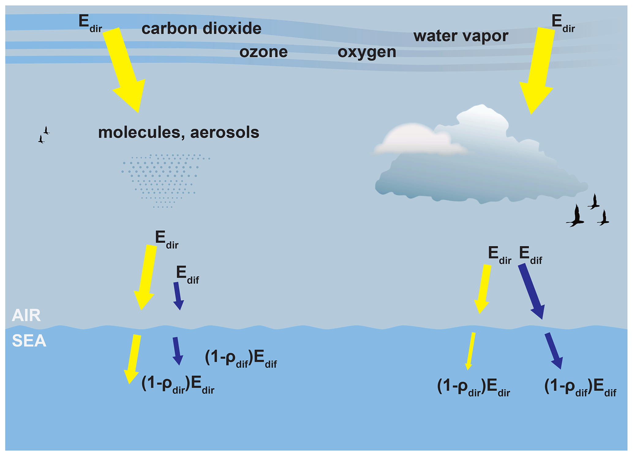
Figure 1Irradiance pathways in OASIM under clear skies (left) and cloudy skies (right): Edir is the direct downwelling irradiance, Edif is the diffuse downwelling irradiance, and ρdir and ρdif are the direct and diffuse surface reflectances, respectively (the size of the arrows approximates the relative contributions; the figure is modified from Fig. 1 of Gregg and Rousseaux, 2017).
OASIM is currently applied in several ocean general circulation models, such as in Poseidon (Gregg, 2002; Gregg and Casey, 2007; Rousseaux and Gregg, 2015) and MOM4 (Gregg and Rousseaux, 2016) of the NASA Global Modelling and Assimilation Office (GMAO), HYCOM (Romanou et al., 2013, 2014) and Russell (Romanou et al., 2014) of the NASA Goddard Institute for Space Studies (GISS), and the MIT OGCM (Dutkiewicz et al., 2015).
OASIM is based on the RADTRAN spectral model developed by Gregg and Carder (1990) for clear-sky conditions, with an upgraded aerosol parameterization scheme, and on the Slingo (1989) parameterization scheme for the spectral cloud transmittance and considers the spectral absorption and scattering of atmospheric gases (ozone, water vapour, oxygen and carbon dioxide). All model parameters (extra-terrestrial solar irradiance, Rayleigh optical thickness and absorption coefficients for the various atmospheric gases) are detailed for each of the 33 bands in Table 2 of GC2009.
In OASIM, gaseous absorption by ozone, oxygen, carbon dioxide and water vapour is resolved before cloud transmittance determination, and aerosol effects are ignored in the presence of clouds. In the clear-sky parameterization scheme, the role of aerosols is described by three parameters: aerosol optical thickness (AOT), single-scattering albedo and asymmetry. These quantities have been applied in GC2009 exploiting Moderate Resolution Imaging Spectroradiometer (MODIS; Remer et al., 2005) data at seven wavelengths ranging from 470 nm to 2.13 µm (for the out-of-range wavelengths, linear extrapolation is performed) from February 2000 to July 2007, extended to 2017 in the present work.
The Slingo model requires four cloud properties as input: cloud cover, cov [%]; cloud liquid water path, LWP [g m−2] (ice clouds are not considered in OASIM); spectral cloud optical thickness, τc(λ) [dimensionless]; and cloud droplet effective radius, re [µm]. The last three properties are linked by the following expression (Slingo, 1989):
where a(λ) and b(λ) are spectral cloud coefficients.
In the original formulation of OASIM presented in GC2009, cov and LWP data are retrieved from the International Satellite Cloud Climatology Project (ISCCP, from June 1986 to July 2002, and the prior climatology), while re is parameterized using MODIS data normalized with mean values obtained from the literature (please refer to GC2009 for details). Specific modelling of the spectral reflectance of sea foam, affecting the transmittance across the air–sea interface, is also included in OASIM (please refer to the Appendix of GC2009).
In addition to the cloud properties necessary for the Slingo model (cloud cover and cloud liquid water path), OASIM requires the following atmospheric input data: surface pressure, sp [mb]; wind speed, ws [m s−1]; relative humidity, rh [%]; precipitable water (absorption by water vapour), wv [cm]; and ozone, oz [DU]. Except for ozone, which was obtained from the multiyear dataset of Total Ozone Mapping Spectrometer (TOMS) sensors (from 1979 to May 1993, hereafter referred to as the TOMS climatology), in GC2009, the other four parameters (sp, ws, rh and wv) were acquired from the National Centers for Environmental Prediction (NCEP 1979 – July 2002; Kalnay et al., 1996) reanalysis dataset. In the present implementation, most of these input data are extracted from the ECMWF ERA-Interim dataset (please refer to Sect. 2.4).
The spatial and temporal resolutions of OASIM are determined by the forcing datasets (i.e. aerosol optical data, cloud property data and atmospheric surface level data). The standard configuration presented in GC2009 is hereby maintained, with a 1∘ horizontal resolution, thereby increasing the temporal frequency to 15 min to resolve the diurnal variability and compare the model output to the temporal resolution of the in situ data considered in the present study. High spatial resolutions and operationally oriented setups are of course possible, provided that forcing data are available: an upgrade in this direction is under investigation based on the ERA5 dataset recently updated and released (C3S, 2017; Hersbach et al., 2020).
2.2 The BGC-Argo float network in the Mediterranean Sea
The BGC-Argo float network represents the first ever near-real-time (NRT) biogeochemical in situ large-scale ocean observing system (Johnson and Claustre, 2016). The technology is relatively recent, and floats equipped with sensors measuring the main biogeochemical and optical parameters have now become operational (Bittig et al., 2019). A BGC-Argo float operates similarly to an Argo float, collecting vertical profiles from 0–1000 m every 1 to 10 d and transmitting NRT data. The profiles are processed with a variable-specific quality control (QC) approach and are available within 24 h after data transmission.
The BGC-Argo floats deployed in the Mediterranean Sea since 2012 are equipped with sensors, which, in addition to the temperature (T), salinity (S) and depth, measure the chlorophyll a (Chl) fluorescence, downward planar irradiance (Ed) at three wavelengths (380, 412 and 490 nm) and downward photosynthetically active radiation (DPAR), which represents the integrated amount of the downward planar irradiance in the visible range, i.e. from 400 to 700 nm. Quality-controlled Chl, T and S NRT data are currently available from the Coriolis data centre (Argo Data Management Team, ADMT).
The photosynthetically active radiation (PAR) must be generally derived by spectrally integrating the scalar irradiance (i.e. the radiance integrated across the complete solid angle) because phytoplankton utilizes light from all directions. In the present case, BGC-Argo sensors measure the downward irradiance integrated in the 400 to 700 nm range: to avoid confusion, the measured quantity is referred to as DPAR.
QC of radiometric data (DPAR and Ed), specifically designed for in situ and remote-sensing ocean colour applications, has been implemented by Organelli et al. (2016). The delayed-mode (DM) QC approach to identify data corruption by biofouling and instrument drift based on tests and procedures has been developed by Organelli et al. (2017). In the present work, a BGC-Argo dataset was adopted covering the period between 2012 and 2017 with 3800 profiles (Fig. 2).
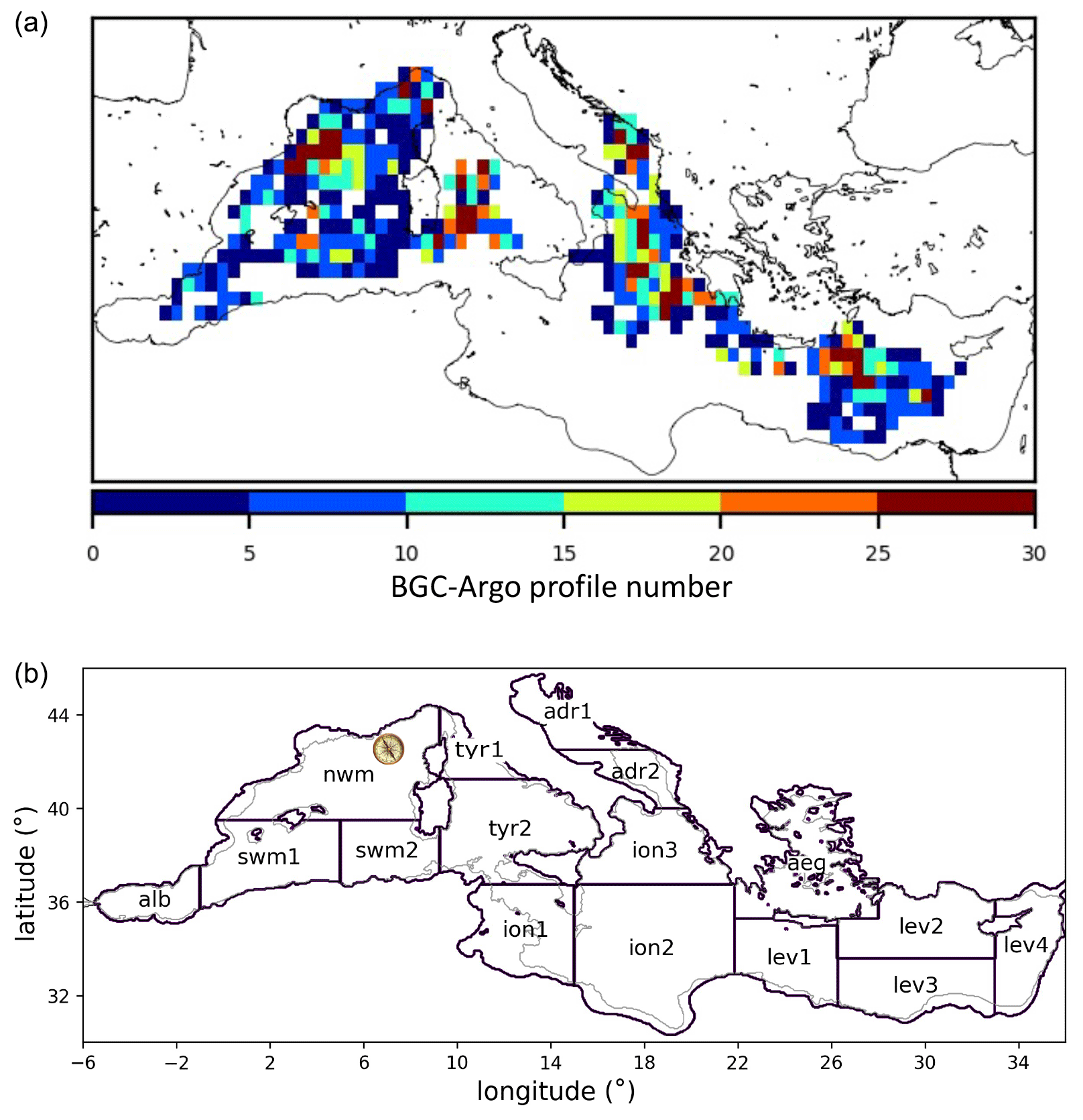
Figure 2(a) Density of the BGC-Argo float profiles in a 0.5∘ × 0.5∘ window covering the period from 2012–2017. (b) Sub-basin division and corresponding area short names as defined in Salon et al. (2019). The compass indicates the BOUSSOLE buoy site (43∘22′ N, 7∘54′ E).
Before comparing model values to observations, the irradiance profiles obtained from floats were extrapolated to the surface with an exponential fitting procedure based on the curve_fit tool of the python package scipy. Further, we required profiles to have at least one measurement in the first 1.5 m depth from sea surface and to have at least four measurements in the first 10 m. In addition, any sub-basin (as defined in Fig. 2) and month containing fewer than five profiles was discarded.
2.3 The BOUSSOLE mooring buoy
The BOUée pour l'acquiSition d'une Série Optique à Long termE (BOUSSOLE) is a long-term mooring station collecting radiometric and bio-optical properties every 15 min from the topmost 10 m of the ocean layer (plus a reference, namely, the above-water measurement of the spectral downward planar irradiance) since 2003 (Antoine et al., 2006). It is located in the Ligurian Sea at 43∘22′ N and 7∘54′ E, approximately 32 nautical miles off the French Riviera coast where the water depth is approximately 2440 m (Fig. 2). The measured quantities include the quality-controlled multispectral (nine bands) downward planar irradiance above the sea surface and DPAR, covering the period from 2003–2012.
2.4 OASIM input data for Mediterranean Sea applications
The input data required by OASIM in the present Mediterranean Sea application are shown in Fig. 3, together with the datasets used for the validation (BOUSSOLE and BGC-Argo). In the setup specific to the Mediterranean Sea, developed within the framework of the BIOPTIMOD project, the variables of the cloud and atmospheric properties are extracted from the European Centre for Medium-Range Weather Forecast (ECMWF) ERA-Interim reanalysis dataset (Dee et al., 2011); further details on their pre-processing are provided in Appendix B. The investigated period ranges from 2004 to 2017, with the input data provided as daily averages and with a spatial resolution of 1∘.
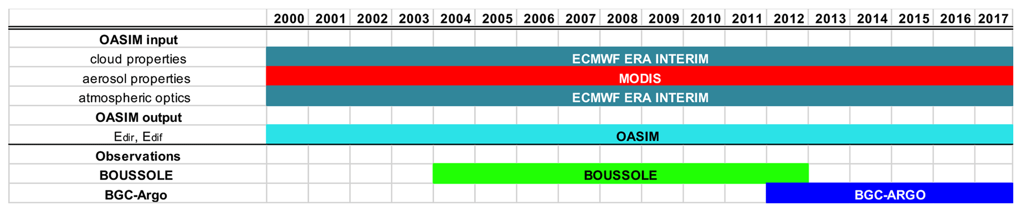
Figure 3Availability of the model input (cloud, aerosol and atmospheric data) and radiometric output data (Edir and Edif) and corresponding observational datasets for the validation in the present work. The acronym definitions are reported in Sect. 2.1, 2.2 and 2.3.
The use of ERA-Interim to force OASIM is motivated by increasing the coherence between the input cloud properties and surface level atmospheric properties, which, in the GC2009 configuration, were provided by two different datasets (ISCCP and NCEP, respectively). Furthermore, considering that the optical module of the MedBFM model will be upgraded as part of the CMEMS operations, ERA-Interim was chosen since ECMWF products are already operational upstream data for the Mediterranean Sea regional production centre of the CMEMS (please refer to Salon et al., 2019). The MODIS data for the period from 2004–2017 are derived in the same way as reported in GC2009 but are extended to 2017.
2.5 OASIM validation in the Mediterranean Sea
Data analysis covered the time period shown in Fig. 3, using datasets from BOUSSOLE (the downward planar irradiance Ed(0−) at 412.5, 442.5, 490, 510, 555, 560, 665, 670 and 681.25 nm, as well as DPAR) and BGC-Argo floats (the downward planar irradiance Ed(0−) at 380, 412 and 490 nm and DPAR).
The notation 0− indicates quantities just below the sea surface with any reflections at the air–sea interface removed, and 0+ is applied for the radiances just above the air–sea interface (the light measured before air–sea transmission occurs).
The OASIM outputs for the irradiance are expressed in watts per quare metres per waveband, while the in situ data for the same parameter are expressed in watts per square centimetre per nanometre. Therefore, before comparison, the units were standardized to watts per square metre per nanometre. Because OASIM simulates data in the range of 350–700 nm centred in 25 nm bins, a linear interpolation was applied to match with measured wavelengths.
Furthermore, the direct (Edir(0−)) and diffuse (Edif(0−)) downward irradiance components simulated by OASIM were summed to compare them to the measurements of the downward planar irradiance sensors installed on the BOUSSOLE and BGC-Argo floats.
DPAR (µmol quanta m−2 s−1) was computed from the OASIM output (in standardized units) by integrating the downward planar irradiance as follows:
where NA is the Avogadro number, h is the Planck constant and c is the speed of light. The definition of DPAR in GC2009 relied on integration with a lower bound of 350 nm, while the BOUSSOLE and BGC-Argo float sensors integrate from 400 nm. The model outputs were standardized according to the observations. To compute DPAR(0−), which is required for a correct comparison to BGC-Argo float sensors, Eq. (2) was adopted by considering Edir(0−) and Edif(0−). Hereafter, Ed(0+) and Ed(0−) indicate the sum of the direct and diffuse downward components.
3.1 ERA-Interim and MODIS atmospheric data analysis
A comparison of the ERA-Interim monthly averaged surface level atmospheric variables at grid points corresponding to the BOUSSOLE mooring buoy and the available observations (sea level pressure, wind speed and relative humidity) by the nearby Côte d'Azur buoy (Météo-France) for the period from 2004–2012 is shown in Fig. 4.
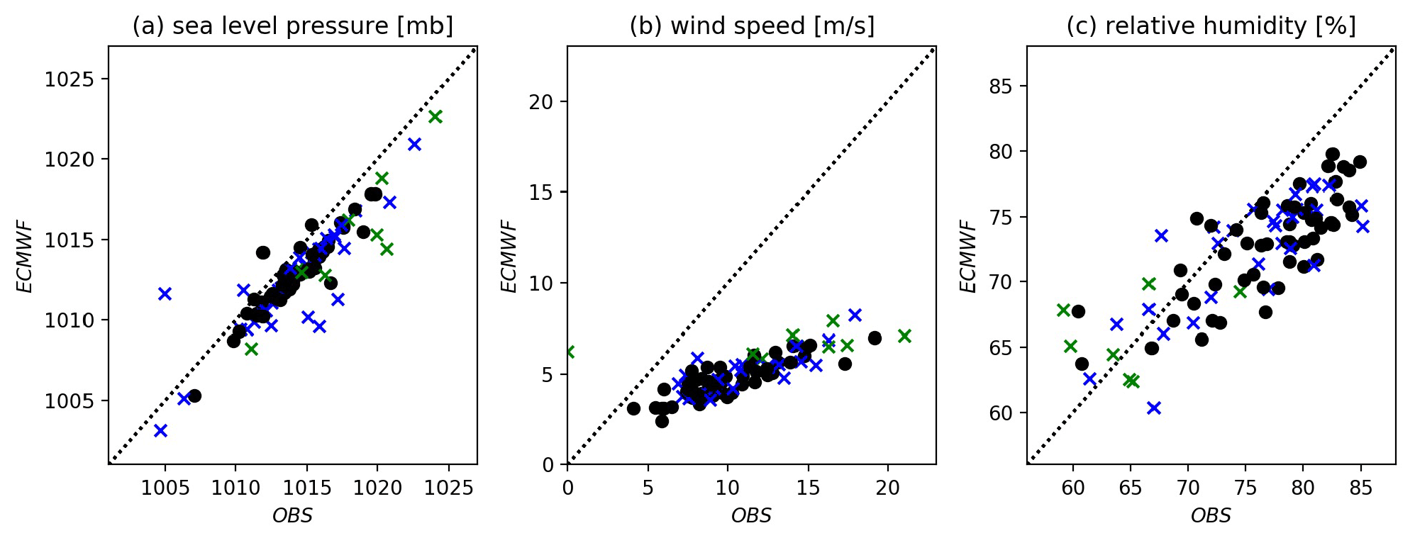
Figure 4Comparison of the ECMWF ERA-Interim monthly averaged data of the sea level pressure (a), wind speed at 10 m (b) and relative humidity (c) and corresponding averages computed from the observations measured by the Côte d'Azur buoy near the BOUSSOLE platform. The symbols represent the different months: January to April (blue crosses), May to October (black dots) and November to December (green crosses).
An overall good agreement is observed for the surface pressure between the ECMWF data and in situ observations, while ERA-Interim underestimates the observed relative humidity (D'Ortenzio et al., 2008). The wind magnitude provided by the Côte d'Azur dataset is much larger than that of the ERA-Interim coarse data at 1∘, as previously reported by Stopa and Cheung (2014) using data from the US National Data Buoy Center. Large differences occur more frequently during the cold season (from November to April). Sensitivity tests to meteorological inputs were performed by Gregg and Carder (1990), showing that pressure and mean wind speed produced differences in surface spectral irradiance of less than 1 % in terms of model error over the 350–700 nm range, much less than air-mass type, visibility and total ozone.
In terms of the spatial distribution, the cloud cover follows a clear seasonal cycle (Fig. 5a), with low values during summer in the eastern sub-basins (ION1, ION2, LEV1, LEV2, LEV3 and LEV3) and a high cover during winter in the northern sub-basins (NWM, TYR1, TYR2, ADR1, ADR2 and AEG). The maximum monthly cloud cover during winter reaches approximately 50 %.
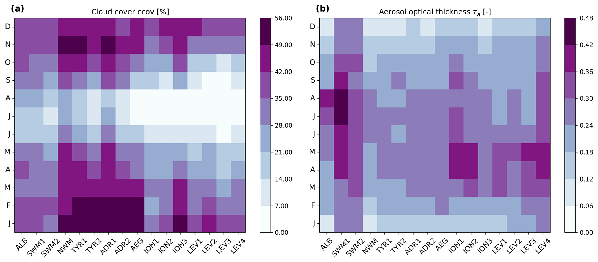
Figure 5ERA-Interim data of the cloud cover (a) and MODIS aerosol optical thickness at 475 nm (b), aggregated spatiotemporally based on the climatological months (y axis) and in the 16 sub-basins (x axis), as shown in Fig. 2.
However, the aerosol optical thickness exhibits a different spatiotemporal pattern. The highest values are localized in the southwestern Mediterranean (SWM1) between July and August, possibly related to Saharan dust events in the area (Varga et al., 2014). High aerosol thickness values are also found in spring (April and May) in the eastern sub-basins (ION1, ION2, LEV3 and LEV4), which also most likely occurs due to aeolian dust transport (Antoine and Nobileau, 2006).
3.2 Validation of OASIM at the BOUSSOLE site
The present OASIM configuration produced data with a 15 min temporal resolution at the global scale on a 1∘ mesh. As an example, the simulated daily cycle averaged over March is shown in Fig. 6. As expected, the measured data present a higher variability than that presented by the model, especially when the intra-monthly frequency is considered. The root mean square difference (RMSD) substantially decreases when considering the monthly average.
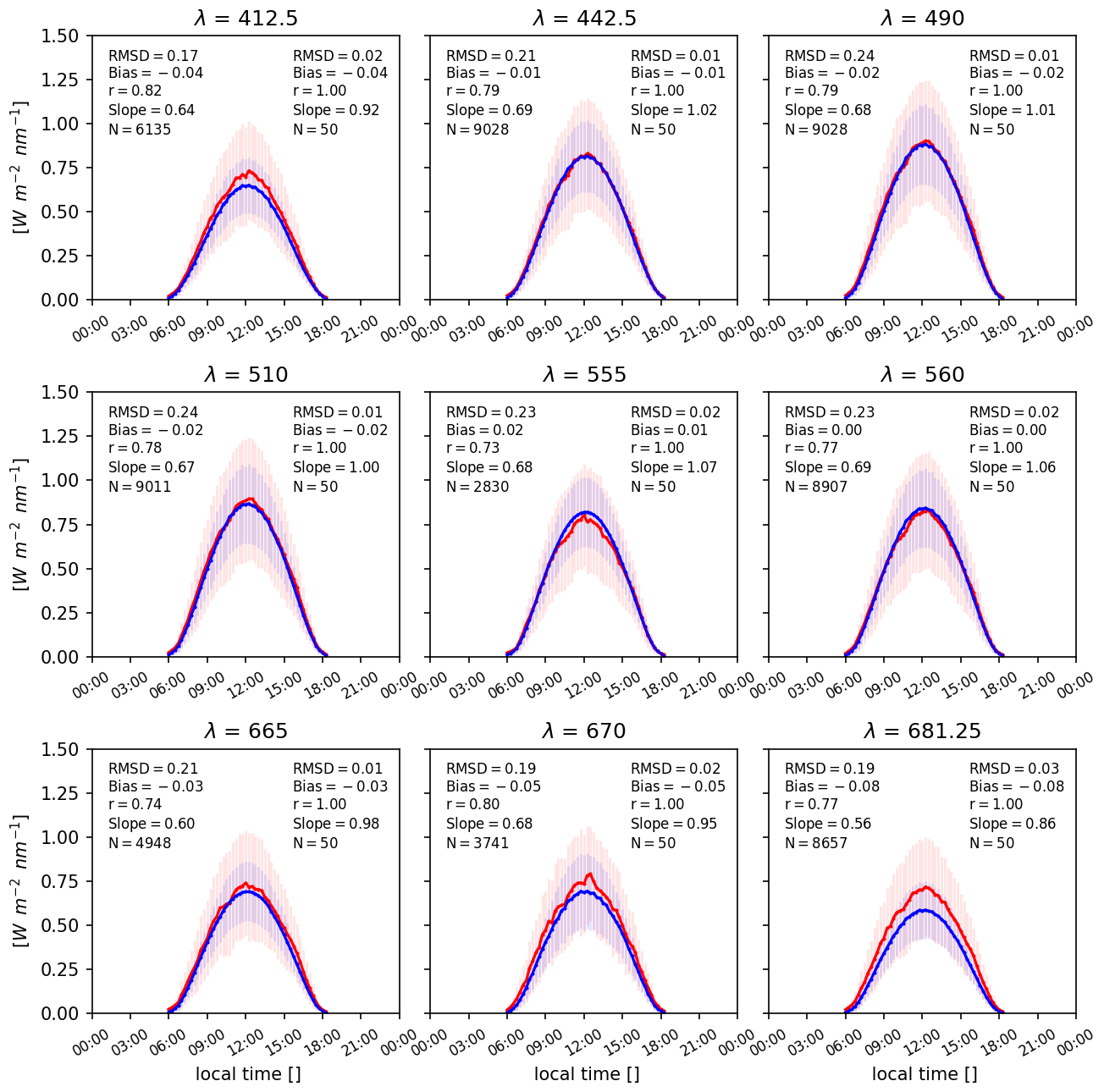
Figure 6Multispectral downward planar irradiance (Ed(λ0−)) simulated by OASIM (blue lines) and measured at BOUSSOLE (red lines). The wavelengths considered are those measured by the BOUSSOLE sensors for the average March data derived from the time series. For each panel, the reported statistics (RMSD, bias, r and regression slope) are related both to the high-frequency signal (with a temporal resolution of 15 min; top left) and to the average day in the considered month (top right). The vertical bars indicate the variance in the monthly averaged values of the average day.
The year-by-year RMSD of the OASIM vs. BOUSSOLE relationship remains steady at approximately 0.2 W m−2 nm−1 (Fig. 7, the red lines). The statistics (Fig. 7, the red dots) indicate a seasonal oscillation: in winter, the high RMSDs and low slopes imply a low prediction skill of the model, whereas in summer, low RMSDs and a slope near 1 indicate a high model skill. Furthermore, an averaged day in each month of the time series (average day per month) was computed, both for the data and model, discretized in 15 min temporal intervals. The same statistics were applied to the averaged data, and the results reveal a reduction in RMSD (Fig. 7, the cyan dots). The average-day-per-month filtering result indicates that the day-by-day variability is responsible for a substantial and consistent part of the uncertainty (please refer to the averaged values shown in Fig. 7).

Figure 7RMSD (left column) and slope (central column) and both indicators (right column) of the relationship between the OASIM and BOUSSOLE downward planar irradiance values (Ed(λ0−)) at the nine wavelengths (λ, in nm) and DPAR. The vertical bars in the left panels of each column are the BOUSSOLE (grey) and model (green) annual averages. The RMSD (W m−2 nm−1) and the slope (dimensionless) are marked in red and black, respectively, with the lines indicating the annual averages and the dots indicating the monthly averages. The monthly statistics are further separated by filtering out the day-by-day variability and are shown as the cyan dots for the RMSD and fuchsia dots for the slope. The averages over the time series are annotated in the panels.
As an additional step, the averaged diurnal cycle grouping all the data in the same month based on the full time series was considered. For example, all the January data from 2004 to 2012 (9 years) were grouped, and the representative climatological day was derived based on a 15 min temporal resolution. In the case of January, at each wavelength and each 15 min interval, there exists a distribution consisting of 31×9 data points (including the data reduction due to sensor failure episodes). In principle, these distributions should be constrained by quite homogeneous conditions, with the same daily zenith angle component, and similar seasonal conditions, i.e. with all the data grouped by the month. Therefore, assuming that a large number of small cumulative perturbations affects the variability, the data should be log-normally distributed.
However, the Kolmogorov–Smirnov test revealed that neither the BOUSSOLE nor the model data distributions are log-normal. In fact, the distances between the accumulated empirical distributions and the reference log-normal distribution were almost always larger than the critical distance (; Bronshtein and Semendyayev, 2013), corresponding to the 5 % probability threshold to reject the null hypothesis (H0 = the two distributions are the same). Moreover, analysis of the skewness and excess kurtosis confirmed that the data and model qualitatively exhibit similar distributions: both are negatively skewed, and the tails decay slower than does a Gaussian distribution (images not shown).
3.3 Validation of OASIM with the BGC-Argo float network
The quality-controlled BGC-Argo float dataset adopted in this work contains radiometric measurements acquired from 10:00 to 14:00 local time. To compare OASIM with these BGC-Argo measurements, a point-by-point match-up analysis was performed, where the closest model output to the float measurement at the surface was selected.
The individual match-ups were then spatiotemporally aggregated based on the climatological months and the defined 16 sub-basins, as shown in Fig. 2, at each of the three wavelengths and for DPAR separately (Figs. 8 to 11).
At 380 nm, the mean values of the model outputs are overall higher than the observations. Apart from the seasonal cycle, a west–east gradient is also observed, with high values in the Eastern Mediterranean, most likely due to the low cloud cover (Fig. 8a, b). Almost all model outputs reveal a positive bias, with the largest differences in the southwestern Mediterranean (SWM2) and southern Adriatic seas (ADR2; up to 0.8 in December), as shown in Fig. 8c. The RMSD exhibits high values in the winter months in the majority of the sub-basins and the lowest values in summer in the Levantine region (LEV1, LEV2 and LEV3; as shown in Fig. 8d).
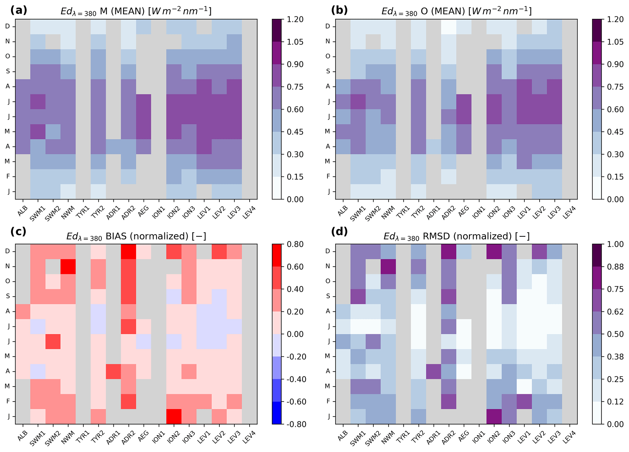
Figure 8Results of the match-up between the model (M) and BGC-Argo float observations (O) for , aggregated spatiotemporally based on the climatological months and 16 sub-basins. The top figures show the mean values of the model (M, a) and observations (O, b). Bias and RMSD are shown in (c) and (d), respectively. The unit is watts per square metre per nanometre, and bias and RMSD are dimensionless due to the normalization by the average values. The grey colour represents the points in space and time for which fewer than five match-ups were available.
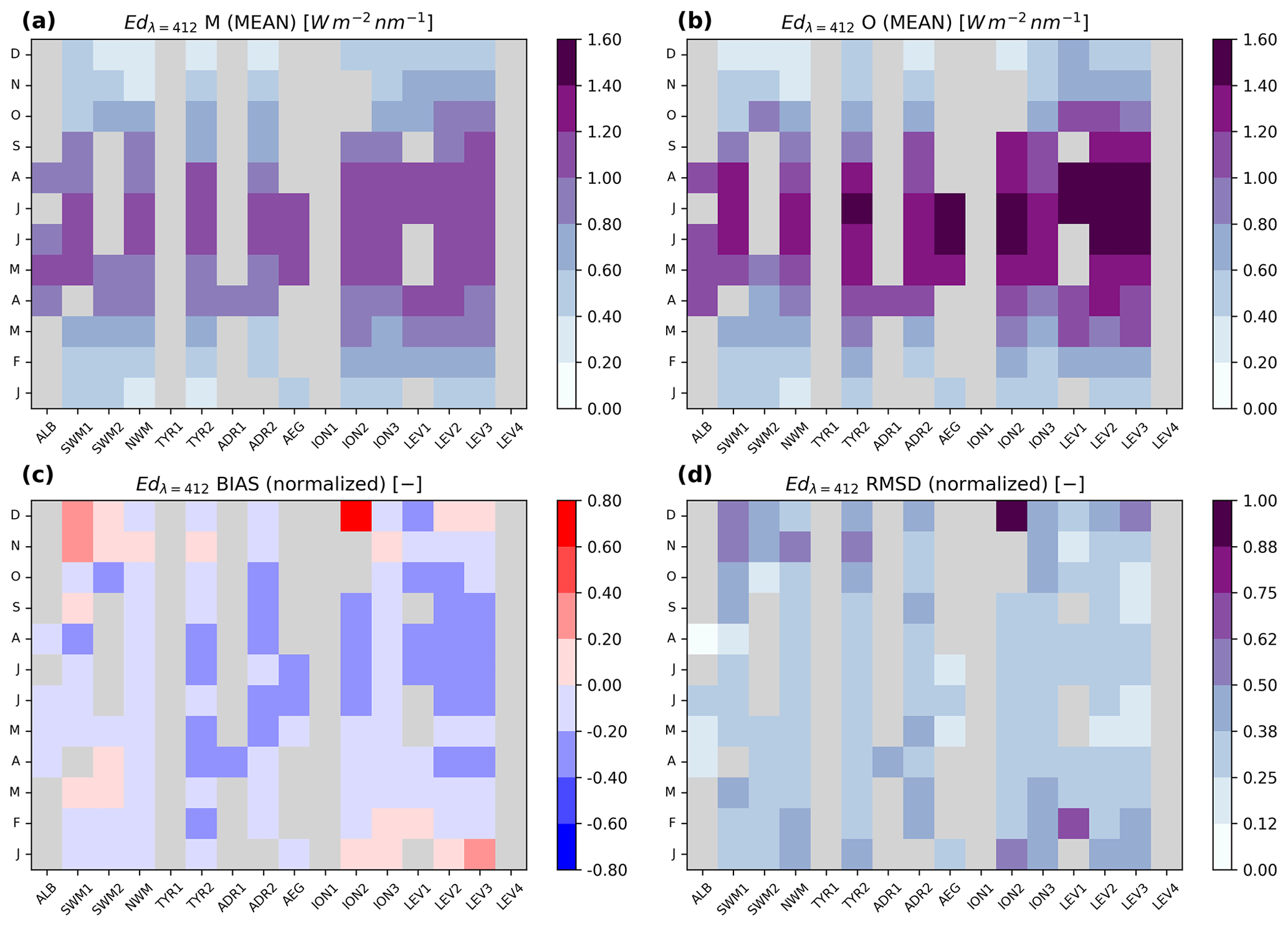
Similar to the findings at the BOUSSOLE site, the model attains low skills with respect to the BGC-Argo float observations at 412 nm, with a less pronounced west–east gradient than that indicated by the observations (Fig. 9a, b). Except for the winter months in the southwestern Mediterranean (SWM1), Ionian (ION2) and Levantine (LEV1, LEV2, LEV3) sub-basins, the bias is negative overall (up to −0.4, as shown in Fig. 9c). The RMSD does not follow a clear pattern, but it is generally close to 0.3, with the highest values in December in the Ionian Sea (ION2), as shown in Fig. 9d.
From late spring to autumn, the bias is predominantly negative from the Tyrrhenian Sea eastwards, varying between 0 and −0.2 (Fig. 10c).
At 490 nm, the model values are higher during winter and early spring months, especially in the western sub-basins (Fig. 10a, b). The highest RMSD values are observed in the southwestern Mediterranean (SWM1) in November and December and in the Levantine region in February (Fig. 10d).
The modelled DPAR values are generally higher than the in situ observations (Fig. 11a, b), with the highest bias and RMSD values observed during the winter period (Fig. 11c, d).
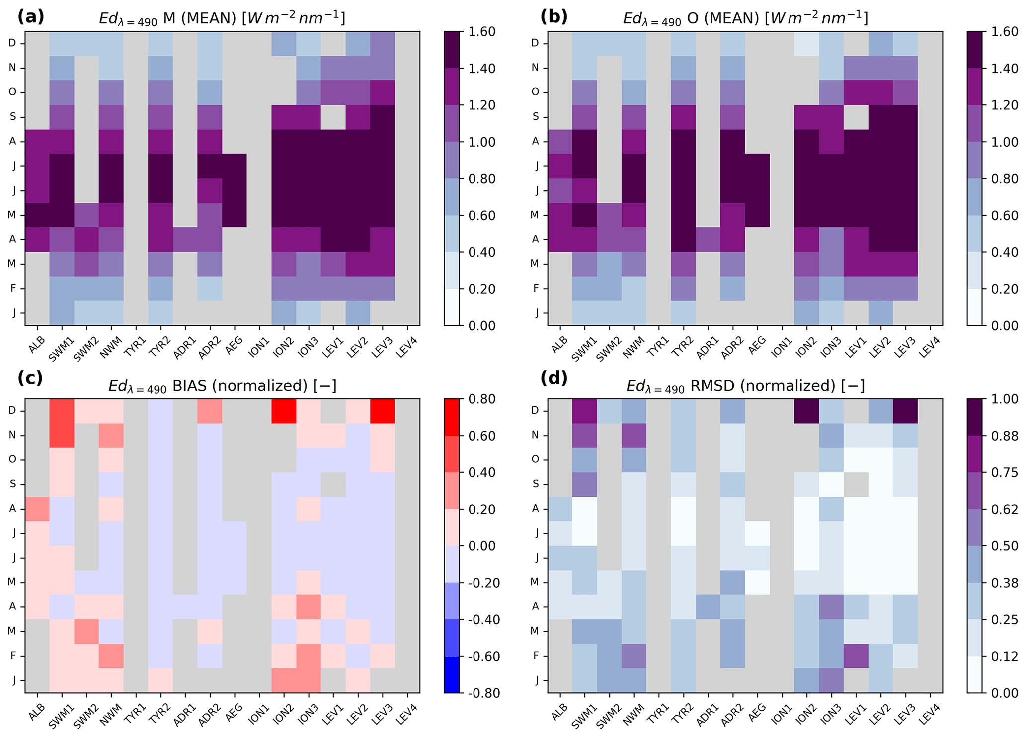
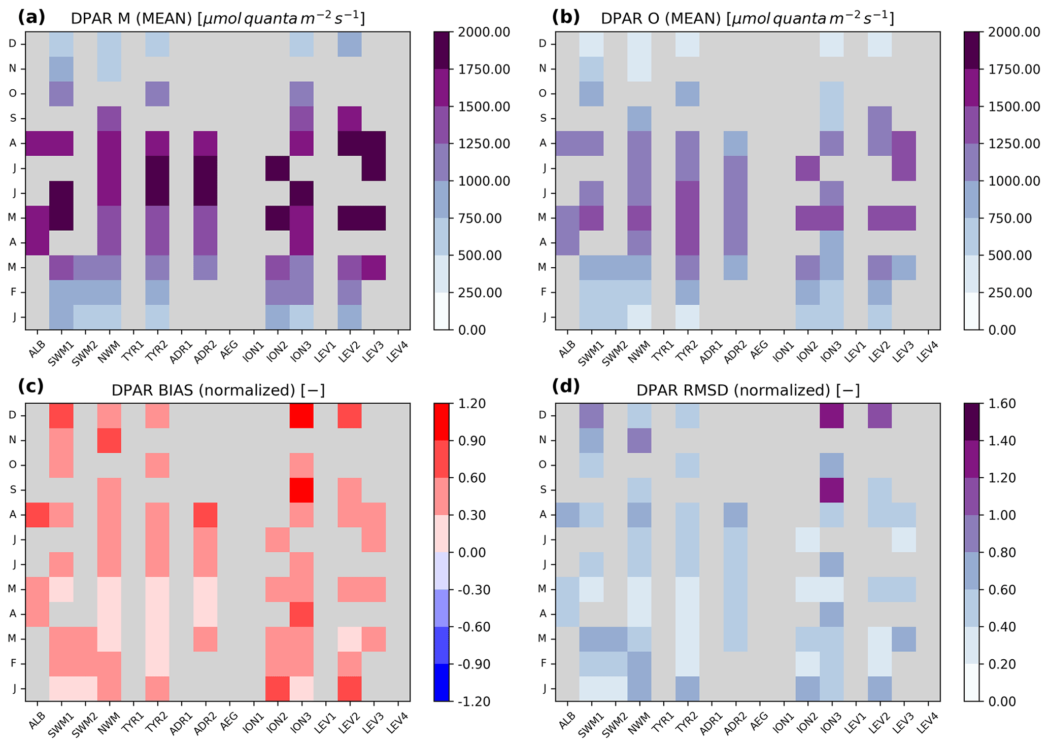
Figure 11Same as Fig. 8 for DPAR; in this case, the mean values are expressed in µmol quanta m−2 s−1.
3.4 Summary of OASIM skills in the Mediterranean Sea
The absolute bias of the comparison of the OASIM outputs to the BOUSSOLE data (Table 1, upper part) is generally lower than 0.1 W m−2 nm−1, and the regression slope approaches 1. In particular, the model vs. the observations reveals a total bias below −20 % of the average measured signal, and on average, the RMSD is approximately 30 %–40 %. The regression slopes are lower than 1, indicating a slight underestimation of the model with respect to the observations in terms of the irradiance maxima, particularly at 412 nm (slope = 0.66), 670 nm (slope = 0.63) and 681.25 nm (slope = 0.62).
Table 1Summary of the model skill compared to the available data from the BOUSSOLE buoy (from 2004 to 2012) and BGC-Argo floats (from 2012 to 2017) for the irradiance (Ed) at the different wavelengths (WLs) and for DPAR. RMSD, bias and y-int are expressed in watts per square metre per nanometre, and in regard to DPAR, the same statistical indicators are expressed in µmol quanta m−2 s−1, while all the other indicators (regression r and slope) are dimensionless, where N is the number of match-ups between the model and observations. For the BOUSSOLE comparison, the numbers in bold font are derived by filtering out the day-to-day variability (i.e. the intra-monthly variability). Given the large number of samples, all statistics are significant (p value < 0.05). For the RMSD and bias, the percentage values normalized by average data are reported in parentheses.
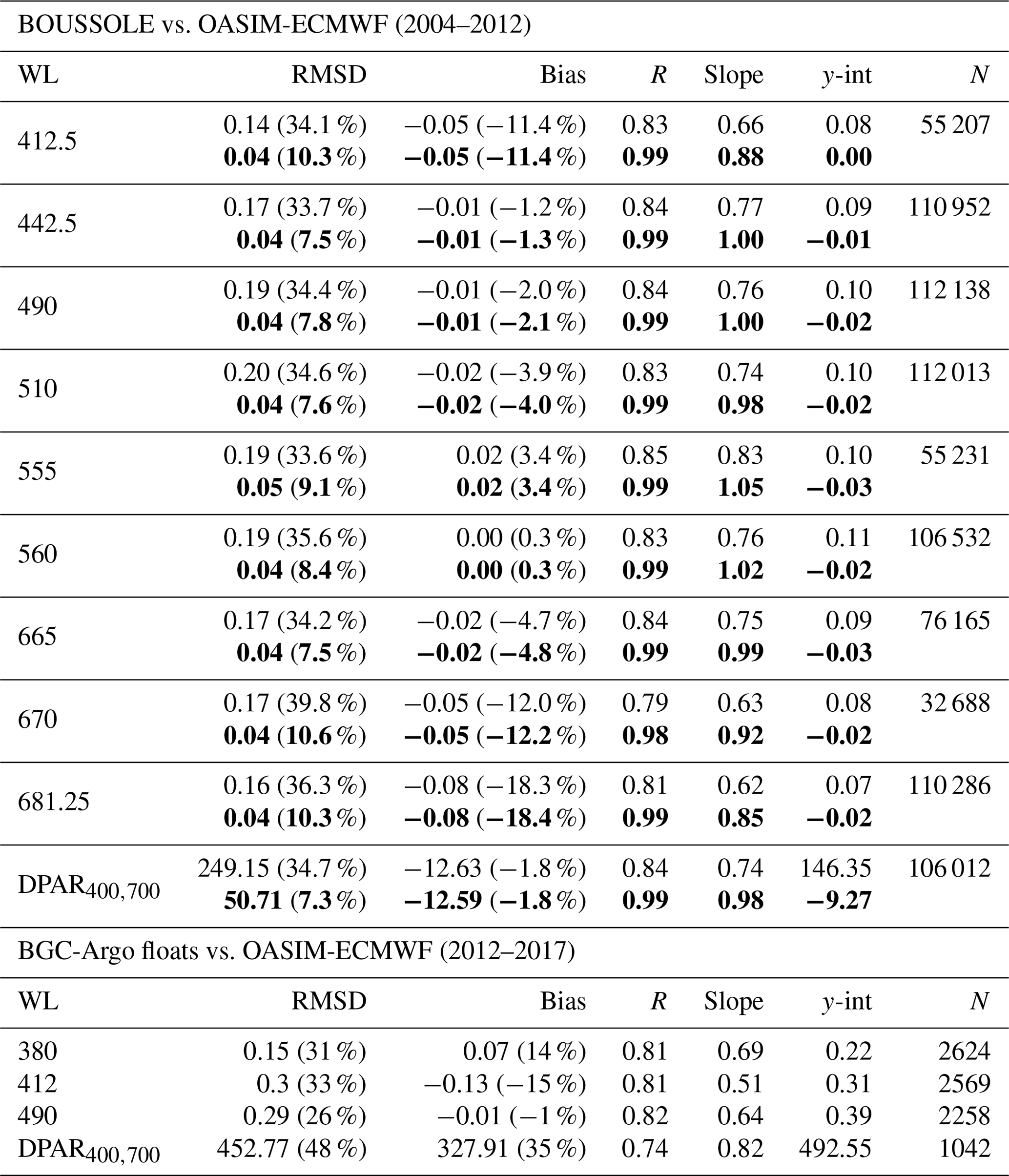
A lower agreement than that between OASIM and BOUSSOLE is observed between OASIM and the BGC-Argo floats (Table 1, lower part), especially in terms of DPAR. Moreover, in this case, the bias is not always negative, being positive only at the 380 nm wavelength and for DPAR. The correlation (R) for indicates a general good agreement between the model and BGC-Argo data (R∼0.8), but the slope is below 0.8. Moreover, similar to OASIM vs. BOUSSOLE, reveals the highest discrepancy at 412 nm, with an RMSD of 0.3 W m−2 nm−1, a bias of −0.13 W m−2 nm−1 and a regression slope of 0.51. The comparison to DPAR indicates a positive bias higher than 300 µmol quanta m−2 s−1, which is high with respect to the BGC-Argo floats than in the BOUSSOLE case. A similar summary analysis performed for was also performed for to estimate the impact of reflection processes at sea atmosphere interface on irradiance (not shown). These processes are regulated by atmospheric parameters shown in Fig. 4: percentual skill metrics indicate that RMSD is only marginally affected, with differences lower than 1 %, while bias for shows differences lower than 5 % with respect to .
3.5 Comparison of OASIM, BOUSSOLE and BGC-Argo floats in the northwestern Mediterranean Sea
Intercomparison of the model outputs and data obtained from the radiometric sensors of the BOUSSOLE buoy and BGC-Argo floats was possible only when the latter were located in the vicinity of the BOUSSOLE buoy in the NW Mediterranean Sea. Different spatial aggregations of profiles surrounding the fixed buoy were tested, ranging from 1∘ (±0.5∘ from the location of the buoy, as shown in Fig. 12) to the whole northwestern Mediterranean sub-basin (NWM), as shown in Fig. 13. In regard to the 1∘ aggregation, up to 10 BGC-Argo profiles were available per month (Fig. 12, number not shown), while for the sub-basin analysis, the number of available profiles ranged from 8 in October to up to 100 in March (Fig. 13, number not shown).
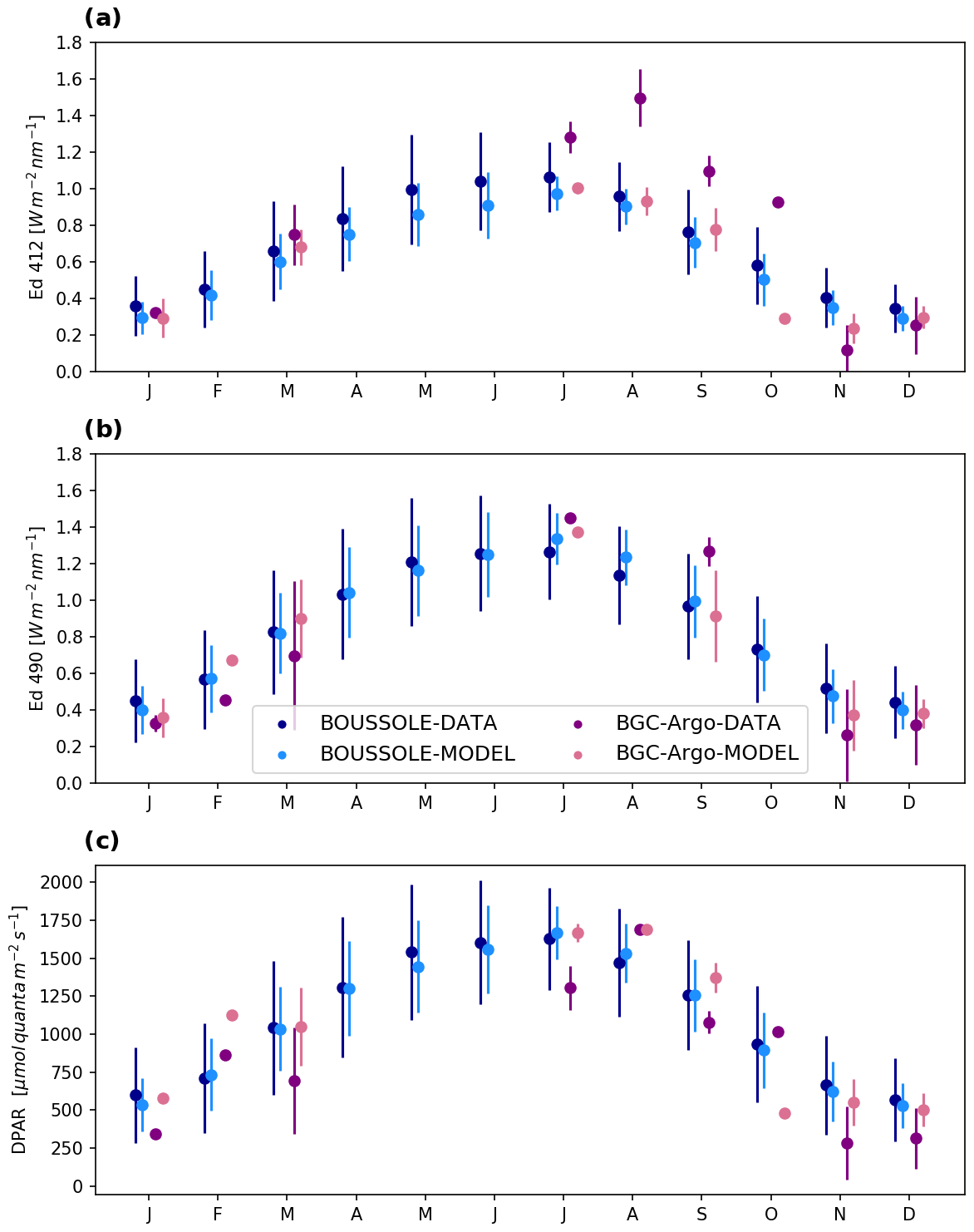
Figure 12Scatter plots of the climatological monthly mean values and standard deviations of the downward irradiance Ed(λ = 412 490 0−) (W m−2 nm−1) and DPAR (µmol quanta m−2 s−1). The blue dots represent the mean values of the measurements at the BOUSSOLE site and the corresponding model outputs, whereas the lilac points display the BGC-Argo values and model means, resulting from the match-up of all available profiles within the 1∘ window (±0.5∘ N/S and W/E from the location of the BOUSSOLE buoy). Note that the points corresponding to each month are horizontally shifted to increase the readability.
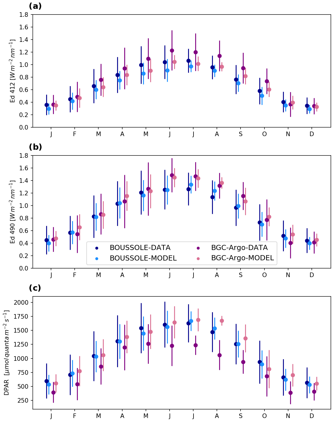
Figure 13Scatter plots of the climatological monthly mean values and standard deviations of the downward irradiance Ed(λ = 412 490 0−) (W m−2 nm−1) and DPAR (µmol quanta m−2 s−1). The blue dots represent the mean values of the measurements at the BOUSSOLE site and the corresponding model outputs, whereas the lilac points display the BGC-Argo values and model means, resulting from the match-up of all available profiles in the northwestern Mediterranean (NWM) sub-basin. Note that the points corresponding to each month are horizontally shifted to increase the readability.
Monthly climatologies were calculated from 2004–2012 for BOUSSOLE and from 2012–2017 for BGC-Argo, with the model values corresponding to the locations of the instruments limited to the model spatial resolution. The BGC-Argo data were extrapolated to the surface, and the considered profiles followed the required conditions, as described in the previous section. The mean values and standard deviations are therefore shown for four different sets of results (Figs. 12 and 13, respectively): the data from the BOUSSOLE buoy and BGC-Argo floats with the corresponding OASIM outputs at 412 and 490 nm (expressed in W m−2 nm−1) and DPAR (expressed in µmol quanta m−2 s−1).
A separate comparison of the two different data sources conveyed an overall good agreement, with higher standard deviation values for the floats (Figs. 12 and 13) than those for the models, revealing a high variability range for the BGC-Argo float data.
The float values that matched with their corresponding OASIM outputs indicated high model outputs at 412 nm, with the largest differences during the summer months, consistent with Fig. 9, with a positive bias of up to 0.2 W m−2 nm−1. The highest bias at the BOUSSOLE site was observed during spring with a similar magnitude (Fig. 13).
The best agreement was generally reached at 490 nm, as is also observed from the NWM column shown in Fig. 10c, especially during the winter months, where the differences between the two assessed platforms decreased to less than 0.1 W m−2 nm−1 (Fig. 13). The largest discrepancy was observed during summer, with the BGC-Argo floats resulting in higher values than those of the BOUSSOLE buoy (up to 0.2 W m−2 nm−1, as shown in Fig. 13).
Consistent with the results shown in Fig. 11, major discrepancies arose when comparing DPAR, where the model values resulted in values much higher than those obtained from the floats, increasing especially during summer (up to 600 µmol quanta m−2 s−1 in August, as shown in Fig. 13).
Such inter- and intra-comparisons of the atmospheric radiative transfer model and available radiometric measurement platforms could also serve as a useful tool to estimate the range of variability when considering optical data from different sources. The spatial aggregation of measurements to the sub-basin level (i.e. a range of up to 10∘) reveals the preservation of the irradiance seasonal variations. However, much remains to be explained in terms of the sources of both variabilities, both between the model and float data, especially when considering DPAR, as well as between the two different sources, such as the floats and fixed buoy.
An extensive comparison of OASIM's temporal and spatial variabilities was performed using the BOUSSOLE and BGC-Argo optical sensor data as references. The results indicated that, in general, the model reproduced the variability in the spectral downward irradiance in the Mediterranean Sea, which depends on the spatiotemporal scale. In particular, considering the OASIM applications within biogeochemical models equipped with a multispectral in-water optical module, the impact will be different according to the specific scale under investigation. In terms of fine temporal scales, it was observed that a large part of the discrepancy expressed by the RMSD occurred due to the day-to-day variability, similar to the findings reported by Somayajula et al. (2018). When this temporal scale is filtered out, the RMSD decreases by half or more. Consistently, the assessed uncertainty (an RMSD of approximately 10 %, bias lower than 10 % and slope >85 %) should be considered in multiannual simulations. In fact, a key parameter such as the primary productivity (strongly affected by the irradiance) exhibits a dominant component of the variance at the seasonal scale (Lazzari et al., 2012), while the day-to-day variability and interannual variability seem to be less important (Di Biagio et al. 2019). In contrast, for short-term forecasts (i.e. 10 d lead time; Salon et al., 2019), the day-to-day variability in the downward irradiance could be relevant. Clearly, to fully investigate the high-frequency RMSD variability, simulations should be refined by increasing the spatial resolution of the model in the region surrounding the BOUSSOLE site (e.g. C3S, 2017; Hersbach et al., 2020).
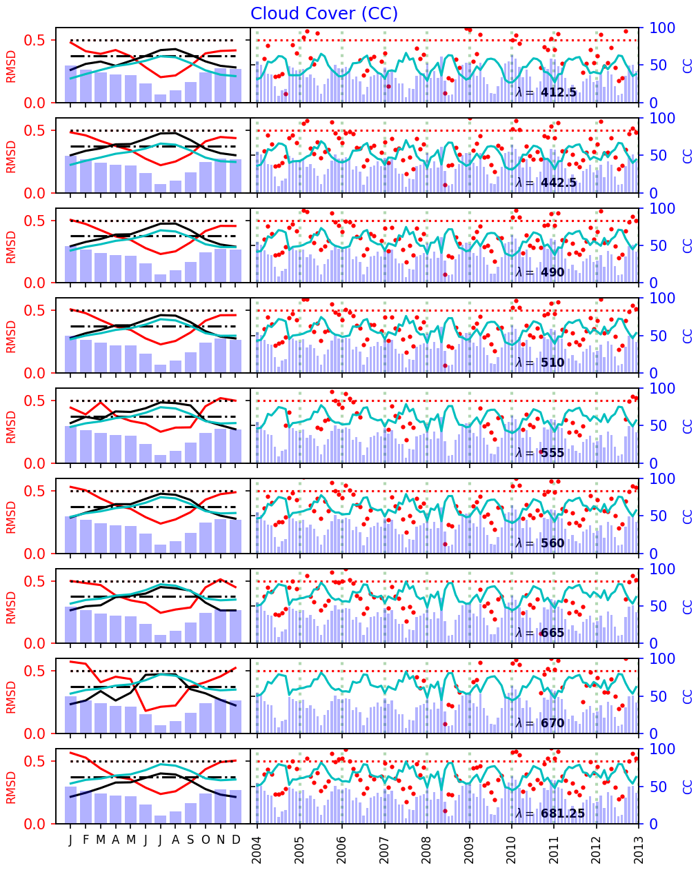
Figure 14Comparison of the OASIM downward irradiance (Ed(λ0−) at the nine wavelengths) to the BOUSSOLE data from 2004 to 2012 in terms of the RMSD and regression slope and their relationship with the ECMWF ERA-Interim cloud cover (CC). The left section of each panel shows the monthly climatology of the RMSD (normalized by its averaged value; red lines and labels) and regression slope (normalized by its averaged value; black line), superimposed on the monthly climatology of the cloud cover (in %, blue bars and labels). Regression slope thresholds at 1 (dotted black line) and 0.75 (dot–dashed black line) are also shown. The right section of each panel shows the monthly means of the time series of the RMSD (red dots, with a 0.5 value; red dotted line), superimposed on the monthly means of the time series of the cloud cover (blue bars and labels). The IND parameter defined in Eq. (3) is also reported (cyan lines) and in all panels varies in the range [0,100].
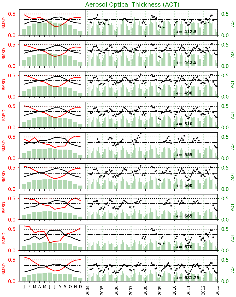
Figure 15Comparison of the OASIM downward irradiance (Ed(λ0−) at the nine wavelengths) to the BOUSSOLE data from 2004 to 2012 in terms of the RMSD and regression slope and their relationship with the MODIS aerosol optical thickness. The left section of each panel shows the monthly climatology of the RMSD (normalized by its averaged value, red lines and labels) and regression slope (normalized by its averaged value, black line), superimposed on the monthly climatology of the aerosol optical thickness (green bars and labels). Regression slope thresholds at 1 (dotted black line) and 0.75 (dot–dashed black line) are also shown. The right section of each panel shows the monthly means of the time series of the regression slope (black dots, with the 1 and 0.75 thresholds shown; dotted and dot–dashed black lines, respectively), superimposed on the monthly means of the time series of the aerosol optical thickness (green bars and labels).
Apart from the diurnal cycle, the cloud cover and aerosols are major drivers in modulating the variability in the downward irradiance, with aerosols being subordinate to the cloud cover. These two input parameters show a high seasonal variability (Figs. 14 and 15). In the Mediterranean area, the cloud cover is high during fall and winter, while the AOT is high during spring and summer (Fig. 5). The winter maximum of the cloud cover corresponds to the maximum RMSD at all wavelengths considered (Fig. 14), while the minimum RMSD occurs in July when the cloud cover is also at its annual minimum. A consistent variability is obtained by computing the regression slope (Figs. 14 and 15). These results are in line with a previous multimodel analysis (Somayajula et al., 2018) indicating that models present a negative bias when the cloud cover is higher than 70 %. Such an underestimation could impact phytoplankton dynamics modelling; thus further analysis should be conducted. The multimodel comparison by Nielsen et al. (2014) revealed that the Slingo liquid-optics model tends to overestimate the cloud optical thickness and therefore underestimates the irradiance.
The presence of a systematic underestimation, following the mechanism described in Nielsen et al. (2014), likely affects all temporal scales. However, in the present study, it was shown that the RMSD and regression slope are greatly improved when filtering out the day-to-day variability. This indicates that high-resolution sampling in OASIM could notably improve the model results. In other words, this implies that reducing the spatiotemporal uncertainty in cloud cover is more important than specific details of the liquid cloud optics parameterizations.
The cloud cover spatial distribution indicates that similar conclusions are obtained based on the model vs. BGC-Argo skills with the results obtained at the BOUSSOLE site; namely, at least for and , the increase in the match between the model and data is modulated by the cloud cover (Figs. 5a, 8, 9 and 10). In contrast, seems to be less influenced by clouds with the exception of the minimum RMSD during summer in the eastern area.
To investigate the balance between direct and diffuse irradiance components, we introduced a further diagnostic (IND) based on their fraction, defined as
where IND is non-dimensional and varies in the interval [0,100]. Recalling that , IND is 0 when and it is 100 when . IND = 50 indicates perfect balance between the two components: . As show in Fig. 14, IND provides a similar interpretation of cloud cover; in fact the model skill is higher when IND is higher and vice versa. This diagnostic indicator could be used to generalize results in regions outside the Mediterranean Sea characterized by lower sun angles, implying a different balance of the direct versus the diffuse component. In these situations, the effect of clouds in increasing RMSD and bias could be even higher. It is worth mentioning that in the present case, since IND covariates with cloud cover, it is difficult to separate the role of clouds from direct versus diffuse irradiance ratio. Nonetheless, IND at 412 nm is lower than all the other wavelengths, and this could explain, at least in part, the lower skill observed at 412 nm.
Apart from cloud dynamics, aerosols play a role in landlocked regions such as the Mediterranean Sea (Papadimas et al., 2008; Nabat et al., 2015). The AOT reveals a variability at least an order of magnitude larger than that of the asymmetry parameter or even more than that of the single-scattering albedo. The minimum RMSD observed in July does not correspond to an extreme AOT value, as observed in the case of the cloud cover. The AOT generally decreases with increasing wavelength (Fig. 15). However, a reduced model skill is observed at 412 and 682.25 nm. The MODIS aerosol data are extrapolated from the seven wavelength channels of the satellite sensors (i.e. 470, 550 and 660 nm in the visible region), which could possibly explain the high uncertainty at 412 nm. In terms of the spatial heterogeneity, comparing the model and BGC-Argo floats (Figs. 5b and 8, 9, and 10), the role of aerosols in the modulation of the model bias and RMSD does not appear to have a clear interpretation.
The low skill at a specific wavelength could be also explained in terms of the wavelength discretization in OASIM: the current model spectral resolution of 25 nm could be refined near 412 and 682.25 nm to investigate whether this would reduce the bias, especially due to the fact that in the present simulations the 412 nm wavelength is at the interface between the band centred at 400 nm and the one centred at 425 nm.
In addition to the seasonal indicators discussed above, the interannual trends of and DPAR were investigated both for the measured data and model results. Given the strong seasonal cycle present in all the properties considered, low-pass filters (i.e. moving averages) were applied to the data before the regression.
The results for both datasets were biased by the gaps in the acquisitions, which introduced spurious trends. Therefore, the focus was on the model inputs instead (ECMWF products and MODIS aerosol data) and the outputs corresponding to a 14-year gap-free time series both in spatial and temporal terms. The model outputs averaged over the Mediterranean Basin indicated a low interannual variability, or at least the procedures adopted based on the low-pass filtering and subsequent regression could not identify clear trends (image not shown). Moreover, the analysis performed demonstrated that the cloud cover interannual variability spans a 2 % range and the AOT at 490 nm exhibits an approximately 10% variability with a maximum in 2009. and DPAR reveal an even lower interannual variability of approximately 1 %.
We assessed the performance of the OASIM radiative model on the Mediterranean Sea for the period 2004–2017, comparing the model outputs with multiplatform reference data. The BOUSSOLE mooring station provides a dataset with a high temporal resolution at a fixed point, while the BGC-Argo floats allow the partial resolution of the spatial variability (certain regions contain no floats), although with a lower spectral resolution than that of BOUSSOLE. The atmospheric multispectral input data provided by OASIM are necessary to resolve the multispectral propagation of light within the water column. Evaluating the uncertainties and the quality of the these input data is fundamental for all the future applications involving bio-optical modelling and constitutes an important starting point to develop assimilation schemes based on bio-optical modelling. The results indicate an overall good agreement between the model outputs and in situ references, highlighting a clear seasonal variability in the model capabilities, with a generally high performance during summer.
The analysis conveys that an important source of discrepancy between the model and data is the intra-monthly variability, which can be ascribed to cloud cover dynamics (the RMSD is reduced with a low cloud cover). The coarse resolution of cloud cover likely affects the model skill at both seasonal and intra-monthly timescales. This is shown by the improvement in model skill at BOUSSOLE when variability between days is filtered out.
Nonetheless, the analysis of the relative contribution of and indicates that the model skill is correlated to their ratio, suggesting that improving the physical description of the radiative processes should be considered. To this end, novel atmospheric models with improved mathematical descriptions of cloud dynamics and advanced numerical solvers may better simulate both clear-sky and cloudy-sky components (Hogan and Bozzo, 2018).
In regard to climatological simulations, the high skill in terms of the monthly averaged irradiance is probably sufficient to properly constrain biogeochemical dynamics, whilst attention should be paid in the case of short-term simulations, when biogeochemical processes such as chlorophyll acclimation exhibit the same timescale as the relatively large fluctuations observed in the RMSD.
In this case, in addition to improved cloud parameterizations, the use of daily resolved aerosol data could possibly reduce the model uncertainties, for example, the EUMETSAT polar multisensor aerosol optical property product (PMAP), available since 2014, or other products provided by the Copernicus Atmosphere Monitoring Services (CAMS). For recent applications see also Bozzo et al. (2020) and Rontu et al. (2020).
Among the wavelengths considered for the downward planar irradiance, 412 and 681 nm appear to result in large uncertainties. However, at this stage, it is not possible to ascertain the reasons for such different skills, and further investigations are required.
| Abbreviation | Full name |
| OASIM | Ocean–Atmosphere Spectral Irradiance Model |
| BOUSSOLE | BOUée pour l'acquiSition d'une Série Optique à Long termE |
| BGC-Argo float | Biogeochemical Argo float |
| DPAR | Downward photosynthetic active radiation |
| OCR-VC | Ocean Colour Radiometry Virtual Constellation |
| CMEMS | Copernicus Marine Environment Monitoring Service |
| MedBFM | Mediterranean Sea biogeochemical operational model system within CMEMS |
| BIOPTIMOD | CMEMS Service Evolution project Integration of novel optical observations in CMEMS biogeochemical models to improve the CMEMS biogeochemical products |
| OLCI | Ocean and Land Colour Instrument |
| ECMWF | European Centre for Medium-Range Weather Forecasts |
| RADTRAN | Spectral atmospheric radiative transfer model |
| AOT | Aerosol optical thickness |
| MODIS | Moderate Resolution Imaging Spectroradiometer |
| ISCCP | International Satellite Cloud Climatology Project |
| TOMS | Total Ozone Mapping Spectrometer |
| C3S | Copernicus Climate Change Service |
| NCEP | National Center for Environmental Prediction |
| ERA-Interim | ECMWF reanalysis period January 1979–August 2019 |
| NRT | Near real time |
| QC | Quality control |
| PAR | Photosynthetic active radiation |
| DM | Delayed mode |
In the present application in the Mediterranean Sea, certain input variables are not directly available from the ERA-Interim dataset in the form required by OASIM, so further processing is needed, as detailed in Table B1.
Table B1Correspondence between the input variables required in OASIM (left column) and the implementation in the Mediterranean Sea (right column), with specific pre-processing steps.
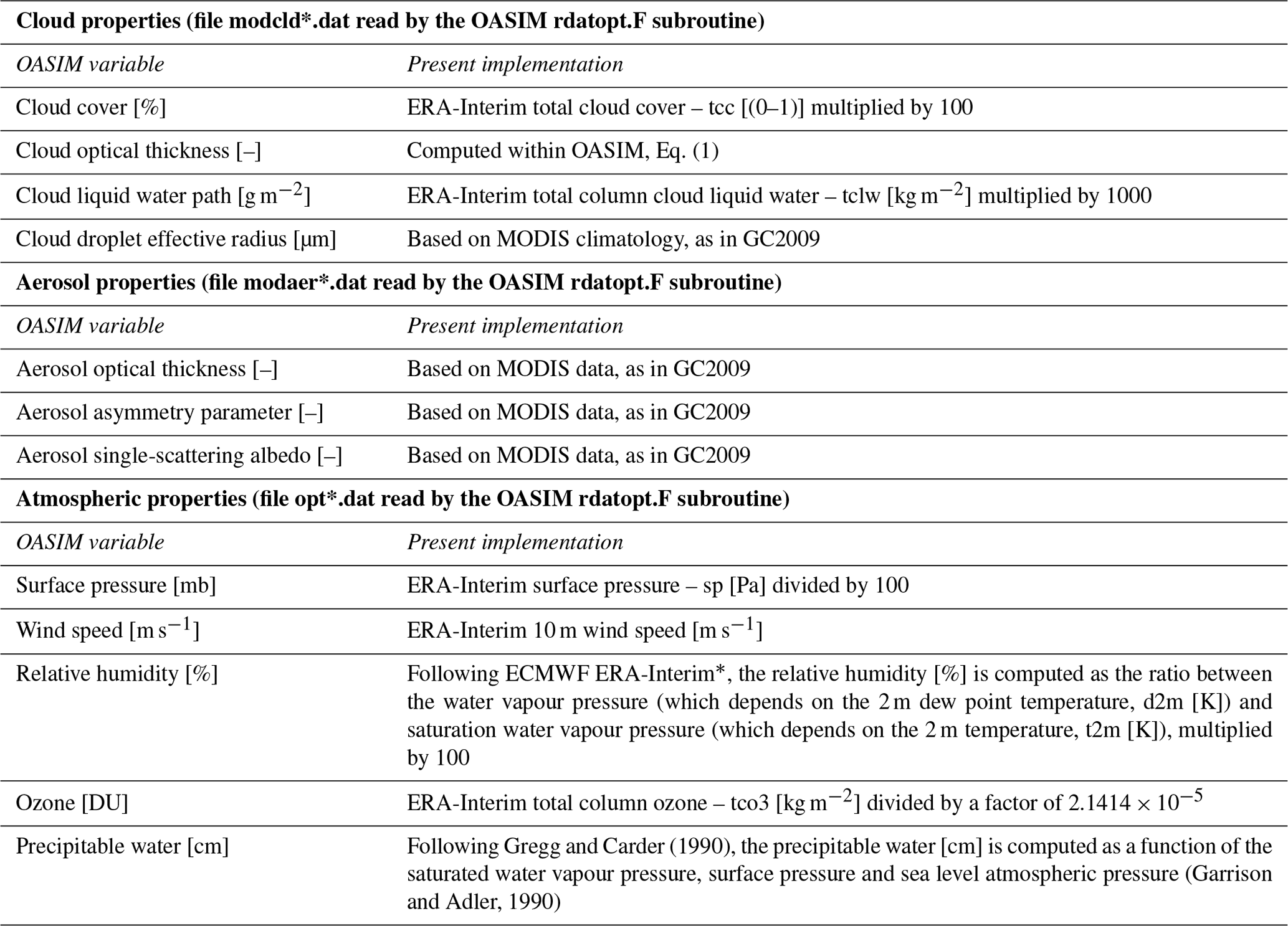
* https://www.ecmwf.int/en/forecasts/datasets/reanalysis-datasets/era-interim (last access: 12 November 2020).
The OASIM Fortran code is publicly downloadable, together with the reference input data, from http://gmao.gsfc.nasa.gov/research/oceanbiology (Gregg, 2020).
Data used in the present study are publicly available from the following sources:
-
ECMWF (Simmon et al., 2007; https://doi.org/10.21957/POCNEX23C6);
-
BOUSSOLE mooring (Antoine and Vellucci, 2020; http://www.obs-vlfr.fr/Boussole/html/project/boussole.php);
-
Mistral site (Bouin and Emzivat, 2020; https://mistrals.sedoo.fr/HyMeX/);
-
BGC-Argo (Argo, 2020; https://doi.org/10.17882/42182#76230).
PL and SS designed the study and the numerical experiments, and PL carried them out supported by WWG. PL and ET performed the model data comparison. VV was in charge of the BOUSSOLE mooring buoy maintenance and performed the quality control of the optical data. DA provided data and funding through the BOUSSOLE project. EO compiled the BGC-Argo database and performed the quality control of the optical data. FDO provided funding and contributed with float deployments. All authors contributed to the interpretation of the results. PL prepared the paper with contributions from all co-authors.
The authors declare that they have no conflict of interest.
The ERA-Interim dataset are published under a Creative Commons Attribution 4.0 International (CC BY 4.0), https://creativecommons.org/licenses/by/4.0/ (last access: 12 November 2020). ECMWF does not accept any liability whatsoever for any error or omission in the data, their availability, or any loss or damage arising from their use.
This article is part of the special issue “Biogeochemistry in the BGC-Argo era: from process studies to ecosystem forecasts (BG/OS inter-journal SI)”. It is a result of the Ocean Sciences Meeting, San Diego, United States, 16–21 February 2020.
This work was performed within the framework of the BIOPTIMOD CMEMS Service Evolution project. CMEMS is implemented by Mercator Ocean International within the framework of a delegation agreement with the European Union.
The authors acknowledge Météo-France for supplying the data and the HyMeX database teams (ESPRI/IPSL and SEDOO/Observatoire Midi-Pyrénées) for their help in accessing the data.
BOUSSOLE is funded by the European Space Agency (ESA), contract 4000119096/17/I-BG, and by the Centre National d'Etudes Spatiales (CNES) with support from the French Oceanographic Fleet (https://doi.org/10.18142/1).
We acknowledge the ECMWF for the ERA-Interim dataset (source: https://www.ecmwf.int, last access: 12 November 2020).
The authors thank Valentina Mosetti (National Institute of Oceanography and Applied Geophysics – OGS) for figure editing.
This work was supported by the BIOPTIMOD CMEMS Service Evolution project. CMEMS is implemented by Mercator Ocean International within the framework of a delegation agreement with the European Union. This study was supported by the following research projects funding BGC-Argo floats: NAOS (funded by the Agence Nationale de la Recherche in the framework of the French “Equipement d'avenir” programme, grant agreement ANR J11R107-F), remOcean (funded by the European Research Council, grant agreement 246777), Argo-Italy (funded by the Italian Ministry of Education, University and Research) and the French Bio-Argo programme (Bio-Argo France; funded by CNES-TOSCA, LEFE Cyber and GMMC).
This paper was edited by Piers Chapman and reviewed by Mark Baird and two anonymous referees.
Antoine, D. and Nobileau, D.: Recent increase of Saharan dust transport over the Mediterranean Sea, as revealed from ocean color satellite (SeaWiFS) observations, J. Geophys. Res.-Atmos., 111, D12214, https://doi.org/10.1029/2005JD006795, 2006.
Antoine, D. and Vellucci, V.: Boussole Mooring, available at: http://www.obs-vlfr.fr/Boussole/html/project/boussole.php, last access: 12 November 2020.
Antoine, D., Chami, M., Claustre, H., D'Ortenzio, F., Morel, A., Bécu, G., Gentili, B., Louis, F., Ras, J., Roussier, E., Scott, A. J., Tailliez, D., Hooker, S. B., Guevel, P., Desté, J. F., Dempsey, C., and Adams, D.: BOUSSOLE: A Joint CNRS-INSU, ESA, CNES and NASA Ocean Color Calibration and Validation Activity, NASA Technical Memorandum N1 2006-214147, NASA/GSFC, Greenbelt, MD, 61 pp., 2006.
Antoine, D., Guevel, P., Deste, J.-F., Becu, G., Louis, F., Scott, A. J., and Bardey, P.: The “BOUSSOLE” Buoy-ANew Transparent to Swell Taut Mooring Dedicated to Marine Optics: Design, Tests, and Performance at Sea, J. Atmos. Ocean. Tech., 25, 968–989, https://doi.org/10.1175/2007JTECHO563.1, 2008.
Antoine, D., Vellucci, V., Banks, A. C., Bardey, P., Bretagnon, M., Bruniquel, V., Deru, A., Hembise Fanton d'Andon, O., Lerebourg, C., Mangin, A., Crozel, D., Victori, S., Kalampokis, A., Karageorgis, A. P., Petihakis, G., Psarra, S., Golbol, M., Leymarie, E., Bialek, A., Fox, N., Hunt, S., Kuusk, J., Laizans, K., and Kanakidou, M.: ROSACE: A Proposed European Design for the Copernicus Ocean Colour System Vicarious Calibration Infrastructure, Remote Sens.-Basel, 12, 1535, https://doi.org/10.3390/rs12101535, 2020.
Argo: Argo float data and metadata from Global Data Assembly Centre (Argo GDAC) – Snapshot of Argo GDAC of August 10st 2020, SEANOE, https://doi.org/10.17882/42182#76230, 2020.
Baird, M. E., Cherukuru, N., Jones, E., Margvelashvili, N., Mongin, M., Oubelkheir, K., Ralph, P. J., Rizwi, F., Robson, B. J., Schroeder, T., Skerratt, J., Steven, A. D. L., and Wild-Allen, K. A.: Remote-sensing reflectance and true colour produced by a coupled hydrodynamic, optical, sediment, biogeochemical model of the Great Barrier Reef, Australia: comparison with satellite data, Environ. Modell. Softw., 78, 79–96, https://doi.org/10.1016/j.envsoft.2015.11.025, 2016.
Bittig, H. C., Maurer, T. L., Plant, J. N., Schmechtig, C., Wong, A. P. S., Claustre, H., Trull, T. W., Udaya Bhaskar, T. V. S., Boss, E., Dall'Olmo, G., Organelli, E., Poteau, A., Johnson, K. S., Hanstein, C., Leymarie, E., Le Reste, S., Riser, S. C., Rupan, A. R., Taillandier, V., Thierry, V., and Xing, X.: A BGC-Argo Guide: Planning, Deployment, Data Handling and Usage, Front. Mar. Sci., 6, 502, https://doi.org/10.3389/fmars.2019.00502, 2019.
Bouin, M.-N. and Emzivat, G.: HyMeX database, available at: https://mistrals.sedoo.fr/HyMeX/, last access: 12 November 2020.
Bozzo, A., Benedetti, A., Flemming, J., Kipling, Z., and Rémy, S.: An aerosol climatology for global models based on the tropospheric aerosol scheme in the Integrated Forecasting System of ECMWF, Geosci. Model Dev., 13, 1007–1034, https://doi.org/10.5194/gmd-13-1007-2020, 2020.
Bronshtein, I. N. and Semendyayev, K. A.: Handbook of mathematics, Springer-Verlag Berlin Heidelberg, LXXXVI, 1164, https://doi.org/10.1007/978-3-540-72122-2, 2013.
C3S: Copernicus Climate Change Service: ERA5: Fifth generation of ECMWF atmospheric reanalyses of the global climate, Copernicus Climate Change Service Climate Data Store (CDS), available at: https://cds.climate.copernicus.eu/cdsapp#!/home (12 November 2020), 2017.
Cossarini, G., Lazzari, P., and Solidoro, C.: Spatiotemporal variability of alkalinity in the Mediterranean Sea, Biogeosciences, 12, 1647–1658, https://doi.org/10.5194/bg-12-1647-2015, 2015.
Cossarini, G., Mariotti, L., Feudale, L., Teruzzi, A., D'Ortenzio, F., Tallandier, V., and Mignot, A.: Towards operational 3D-Var assimilation of chlorophyll Biogeochemical-Argo float data into a biogeochemical model of the Mediterranean Sea, Ocean Model., 133, 112–128, https://doi.org/10.1016/j.ocemod.2018.11.005, 2019.
Dee, D. P., Uppala, S. M., Simmons, A. J., Berrisford, P., Poli, P., Kobayashi, S., Andrae, U., Balmaseda, M. A., Balsamo, G., Bauer, P., Bechtold, P., Beljaars, A. C., van de Berg, L., Bidlot, J., Bormann, N., Delsol, C., Dragani, R., Fuentes, M., Geer, A. J., Haimberger, L., Healy, S. B., Hersbach, H., Hólm, E. V., Isaksen, L., Kållberg, P., Köhler, M., Matricardi, M., McNally, A. P., Monge-Sanz, B. M., Morcrette, J., Park, B., Peubey, C., de Rosnay, P., Tavolato, C., Thépaut, J., and Vitart, F.: The ERA-Interim reanalysis: configuration and performance of the data assimilation system, Q. J. Roy. Meteor. Soc., 137, 553–597, https://doi.org/10.1002/qj.828, 2011.
Di Biagio, V., Cossarini, G., Salon, S., Lazzari, P., Querin, S., Sannino, G., and Solidoro, C.: Temporal scales of variability in the Mediterranean Sea ecosystem: Insight from a coupled model, J. Marine Syst., 197, 103176, https://doi.org/10.1016/j.jmarsys.2019.05.002, 2019.
Donlon, C., Berruti, B., Buongiorno, A., Ferreira, M.-H., Féménias, P., Frerick, J., Goryl, P., Klein, U., Laur, H., Mavrocordatos, C., Nieke, J., Rebhan, H., Seitz, B., Stroede, J., and Sciarra, R.: The Global Monitoring for Environment and Security (GMES) Sentinel-3 mission, Remote Sens. Environ., 120, 37–57, https://doi.org/10.1016/j.rse.2011.07.024, 2012.
D'Ortenzio, F., Antoine, D., and Marullo, S.: Satellite-driven modelling of the upper ocean mixed layer and air-sea CO2 flux in the Mediterranean Sea, Deep-Sea Res. Pt. I, 55, 405–434, https://doi.org/10.1016/j.dsr.2007.12.008, 2008.
Dowd, M., Jones, E., and Parslow, J.: A statistical overview and perspectives on data assimilation for marine biogeochemical models, Environmetrics, 25, 203–213, https://doi.org/10.1002/env.2264, 2014.
Dutkiewicz, S., Hickman, A. E., Jahn, O., Gregg, W. W., Mouw, C. B., and Follows, M. J.: Capturing optically important constituents and properties in a marine biogeochemical and ecosystem model, Biogeosciences, 12, 4447–4481, https://doi.org/10.5194/bg-12-4447-2015, 2015.
Garrison, J. D. and Adler, G. P.: Estimation of precipitable water over the United States for application to the division of solar radiation into its direct and diffuse components, Sol. Energy, 44, 225–241, https://doi.org/10.1016/0038-092X(90)90151-2, 1990.
Gregg, W. W.: A coupled ocean-atmosphere radiative model for global ocean biogeochemical models, in: NASA Global Modeling and Assimilation Series, edited by: Suarez, M., NASA Technical Memorandum 2002-104606, Greenbelt, Maryland, USA, 33 pp., 2002.
Gregg, W. W.: OASIM model, available at: https://gmao.gsfc.nasa.gov/research/oceanbiology/, last access: 12 November 2020.
Gregg, W. W. and Carder, K. L.: A simple spectral solar irradiance model for cloudless maritime atmospheres, Limnol. Oceanogr., 35, 1657–1675, https://doi.org/10.4319/lo.1990.35.8.1657, 1990.
Gregg, W. W. and Casey, N. W.: Modeling coccolithophores in the global oceans, Deep-Sea Res. Pt. II, 54, 447–477, https://doi.org/10.1016/j.dsr2.2006.12.007, 2007.
Gregg, W. W. and Casey, N. W.: Skill assessment of a spectral ocean-atmosphere radiative model, J. Marine Syst., 76, 49–63, https://doi.org/10.1016/j.jmarsys.2008.05.007, 2009.
Gregg, W. W. and Rousseaux, C. S.: Directional and Spectral Irradiance in Ocean Models: Effects on Simulated Global Phytoplankton, Nutrients, and Primary Production, Front. Mar. Sci., 3, 240, https://doi.org/10.3389/fmars.2016.00240, 2016.
Gregg, W. W. and Rousseaux, C. S.: Simulating PACE Global Ocean Radiances, Front. Mar. Sci., 4, 60, https://doi.org/10.3389/fmars.2017.00060, 2017.
Hersbach, H., Bell, B., Berrisford, P., Hirahara, S., Horányi, A., Muñoz-Sabater, J., Nicolas, J., Peubey, C., Radu, R., and Schepers, D.: The ERA5 global reanalysis, Q. J. Roy. Meteor. Soc., 146, 1999–2049, https://doi.org/10.1002/qj.3803, 2020.
Hogan, R. J. and Bozzo, A.: A flexible and efficient radiation scheme for the ECMWF model, J. Adv. Model. Earth Sy., 10, 1990–2008, https://doi.org/10.1029/2018MS001364, 2018.
Johnson, K. S. and Claustre, H.: Bringing biogeochemistry into the Argo age, Eos, 97, 1–12, https://doi.org/10.1029/2016EO062427, 2016.
Jones, E. M., Baird, M. E., Mongin, M., Parslow, J., Skerratt, J., Lovell, J., Margvelashvili, N., Matear, R. J., Wild-Allen, K., Robson, B., Rizwi, F., Oke, P., King, E., Schroeder, T., Steven, A., and Taylor, J.: Use of remote-sensing reflectance to constrain a data assimilating marine biogeochemical model of the Great Barrier Reef, Biogeosciences, 13, 6441–6469, https://doi.org/10.5194/bg-13-6441-2016, 2016.
Kalnay, E., Kanamitsu, M., Kistler, R., Collins, W., Deaven, D., Gandin, L., Iredell, M., Saha, S., White, G., Woollen, J., Zhu, Y., Chelliah, M., Ebisuzaki, W., Higgins, W., Janowiak, J., Mo, K. C., Ropelewski, C., Wang, J., Leetmaa, A., Reynolds, R., Jenne, R., and Joseph, D.: The NCEP/NCAR 40-year reanalysis project, B. Am. Meteorol. Soc., 77, 437–471, https://doi.org/10.1175/1520-0477(1996)077<0437:TNYRP>2.0.CO;2, 1996.
Lazzari, P., Teruzzi, A., Salon, S., Campagna, S., Calonaci, C., Colella, S., Tonani, M., and Crise, A.: Pre-operational short-term forecasts for Mediterranean Sea biogeochemistry, Ocean Sci., 6, 25–39, https://doi.org/10.5194/os-6-25-2010, 2010.
Lazzari, P., Solidoro, C., Ibello, V., Salon, S., Teruzzi, A., Béranger, K., Colella, S., and Crise, A.: Seasonal and inter-annual variability of plankton chlorophyll and primary production in the Mediterranean Sea: a modelling approach, Biogeosciences, 9, 217–233, https://doi.org/10.5194/bg-9-217-2012, 2012.
Lazzari, P., Solidoro, C., Salon, S., and Bolzon, G.: Spatial variability of phosphate and nitrate in the Mediterranean Sea: a modelling approach, Deep-Sea Res. Pt. I, 108, 39–52, https://doi.org/10.1016/j.dsr.2015.12.006, 2016.
Leymarie, E., Penkerc'h, C., Vellucci, V., Lerebourg, C., Antoine, D., Boss, E., Lewis, M., D'Ortenzio, F., and Claustre, H.: ProVal: A new autonomous profiling float for high quality radiometric measurements, Front. Mar. Sci., 5, 437, https://doi.org/10.3389/fmars.2018.00437, 2018.
Nabat, P., Somot, S., Mallet, M., Michou, M., Sevault, F., Driouech, F., Meloni, D., di Sarra, A., Di Biagio, C., Formenti, P., Sicard, M., Léon, J.-F., and Bouin, M.-N.: Dust aerosol radiative effects during summer 2012 simulated with a coupled regional aerosol–atmosphere–ocean model over the Mediterranean, Atmos. Chem. Phys., 15, 3303–3326, https://doi.org/10.5194/acp-15-3303-2015, 2015.
Nielsen, K. P., Gleeson, E., and Rontu, L.: Radiation sensitivity tests of the HARMONIE 37h1 NWP model, Geosci. Model Dev., 7, 1433–1449, https://doi.org/10.5194/gmd-7-1433-2014, 2014.
Organelli, E., Claustre, H., Bricaud, A., Schmechtig, C., Poteau, A., Xing, X., Prieur, L., D'Ortenzio, F., Dall'Olmo, G., and Vellucci, V.: A novel near real-time quality-control procedure for radiometric profiles measured by Bio-Argo floats: protocols and performances, J. Atmos. Ocean. Tech., 33, 937–951, https://doi.org/10.1175/JTECH-D-15-0193.1, 2016.
Organelli, E., Barbieux, M., Claustre, H., Schmechtig, C., Poteau, A., Bricaud, A., Boss, E., Briggs, N., Dall'Olmo, G., D'Ortenzio, F., Leymarie, E., Mangin, A., Obolensky, G., Penkerc'h, C., Prieur, L., Roesler, C., Serra, R., Uitz, J., and Xing, X.: Two databases derived from BGC-Argo float measurements for marine biogeochemical and bio-optical applications, Earth Syst. Sci. Data, 9, 861–880, https://doi.org/10.5194/essd-9-861-2017, 2017.
Papadimas, C. D., Hatzianastassiou, N., Mihalopoulos, N., Querol, X., and Vardavas, I.: Spatial and temporal variability in aerosol properties over the Mediterranean basin based on 6-year (2000–2006) MODIS data, J. Geophys. Res.-Atmos., 113, D11205, https://doi.org/10.1029/2007JD009189, 2008.
Remer, L. A., Kaufman, Y. J., Tanre, D., Mattoo, S., Chu, D. A., Martins, J. V., Li, R.-R., Ichoku, C., Levy, R. C., Kleidman, R. G., Eck, T. F., Vermote, E., and Holben, B. N.: The MODIS aerosol algorithm, products and validation, J. Atmos. Sci., 62, 947–973, https://doi.org/10.1175/JAS3385.1, 2005.
Romanou, A., Gregg, W. W., Romanski, J., Kelley, M., Bleck, R., Healy, R., Nazarenko, L., Russell, G., Schmidt, G. A., Sun, S., and Tausnev, N.: Natural air-sea flux of CO2 in simulations of the NASA-GISS climate model: sensitivity to the physical ocean model formulation, Ocean Model., 66, 26–44, https://doi.org/10.1016/j.ocemod.2013.01.008, 2013.
Romanou, A., Romanski, J., and Gregg, W. W.: Natural ocean carbon cycle sensitivity to parameterizations of the recycling in a climate model, Biogeosciences, 11, 1137–1154, https://doi.org/10.5194/bg-11-1137-2014, 2014.
Rontu, L., Gleeson, E., Martin Perez, D., Pagh Nielsen, K., and Toll, V.: Sensitivity of Radiative Fluxes to Aerosols in the ALADIN-HIRLAM Numerical Weather Prediction System, Atmosphere, 11, 205, https://doi.org/10.3390/atmos11020205, 2020.
Rousseaux, C. S. and Gregg, W. W.: Recent decadal trends in global phytoplankton composition, Global Biogeochem. Cy., 29, 1674–1688, https://doi.org/10.1002/2015GB005139, 2015.
Salon, S., Cossarini, G., Bolzon, G., Feudale, L., Lazzari, P., Teruzzi, A., Solidoro, C., and Crise, A.: Novel metrics based on Biogeochemical Argo data to improve the model uncertainty evaluation of the CMEMS Mediterranean marine ecosystem forecasts, Ocean Sci., 15, 997–1022, https://doi.org/10.5194/os-15-997-2019, 2019.
Slingo, A.: A GCM Parameterization for the Shortwave Radiative Properties of Water Clouds, J. Atmos. Sci., 46, 1419–1427, https://doi.org/10.1175/1520-0469(1989)046<1419:AGPFTS>2.0.CO;2, 1989.
Simmons, A., Uppala, S., Dee, D., Kobayashi, S.: ERA-Interim: New ECMWF reanalysis products from 1989 onwards, https://doi.org/10.21957/POCNEX23C6, 2007.
Somayajula, S. A., Devred, E., Bélanger, S., Antoine, D., Vellucci, V., and Babin, M.: Evaluation of sea-surface photosynthetically available radiation algorithms under various sky conditions and solar elevations, Appl. Optics, 57, 3088–3105, https://doi.org/10.1364/AO.57.003088, 2018.
Stopa, J. E. and Cheung, K. F.: Intercomparison of wind and wave data from the ECMWF Reanalysis Interim and the NCEP Climate Forecast System Reanalysis, Ocean Model., 75, 65–83, https://doi.org/10.1016/j.ocemod.2013.12.006, 2014.
Teruzzi, A., Dobricic, S., Solidoro, C., and Cossarini, G.: A 3D variational assimilation scheme in coupled transport-biogeochemical models: Forecast of Mediterranean biogeochemical properties, J. Geophys. Res.-Oceans, 119, 200–217, https://doi.org/10.1002/2013JC009277, 2014.
Teruzzi, A., Bolzon, G., Salon, S., Lazzari, P., Solidoro, C., and Cossarini, G.: Assimilation of coastal and open sea biogeochemical data to improve phytoplankton modelling in the Mediterranean Sea, Ocean Model., 132, 46–60, https://doi.org/10.1016/j.ocemod.2018.09.007, 2018.
Teruzzi, A., Di Cerbo, P., Cossarini, G., Pascolo, E., and Salon, S.: Parallel implementation of a data assimilation scheme for operational oceanography: The case of the MedBFM model system, Comput. Geosci., 124, 103–114, https://doi.org/10.1016/j.cageo.2019.01.003, 2019.
Varga, G., Újvári, G., and Kovács, J.: Spatiotemporal patterns of Saharan dust outbreaks in the Mediterranean Basin, Aeolian Res., 15, 151–160, https://doi.org/10.1016/j.aeolia.2014.06.005, 2014.