Multi-decadal variability in seasonal mean sea level along the North Sea coast

Seasonal deviations from annual-mean sea level in the North Sea region show a large low-frequency component with substantial variability at decadal and multi-decadal timescales. In this study, we quantify low-frequency variability in seasonal deviations from annual-mean sea level and look for drivers of this variability. The amplitude, as well as the temporal evolution of this multi-decadal variability shows substantial variations over the North Sea region, and this spatial pattern is similar to the well-known pattern of the influence of winds and pressure changes on sea level at higher frequencies. The largest low-frequency signals are found in the German Bight and along the Norwegian coast. We find that the variability is much stronger in winter and autumn than in other seasons and that this winter and autumn variability is predominantly driven by wind and sea-level pressure anomalies which are related to large-scale atmospheric patterns. For the spring and summer seasons, this atmospheric forcing explains a smaller fraction of the observed variability.

Large-scale atmospheric patterns have been derived from a principal component analysis of sea-level pressure. The first principal component of sea-level pressure over the North Atlantic Ocean, which is linked to the North Atlantic Oscillation (NAO), explains the largest fraction of winter-mean variability for most stations, while for some stations, the variability consists of a combination of multiple principal components.

The low-frequency variability in season-mean sea level can manifest itself as trends in short records of seasonal sea level. For multiple stations around the North Sea, running-mean 40-year trends for autumn and winter sea level often exceed the long-term trends in annual mean sea level, while for spring and summer, the seasonal trends have a similar order of magnitude as the annual-mean trends. Removing the variability explained by atmospheric variability vastly reduces the seasonal trends, especially in winter and autumn.

1 Introduction

Analyses of sea-level records, with respect to deducing trends and their causes, as well as sea-level projections commonly focus on annual-mean values (Piecuch et al., 2016; Slangen et al., 2017; Wahl et al., 2013). However, next to interannual sea-level variability, which is captured by annual-mean sea level, season-mean sea level (e.g. winter mean or summer mean) could have its own variability on top of the annual-mean variability. In this study, we quantify this seasonal sea-level variability in the North Sea region and look into its causes. It has already been demonstrated that for the southwestern North Sea, different seasons show distinct variability patterns: Dangendorf et al. (2013) demonstrated the difference between annual-mean and seasonal variability from the Cuxhaven tide-gauge record. In particular, variability in spring and summer (which were broadly similar) diverged strongly from the autumn and winter seasons. Hence, variability in annual-mean sea level is not necessarily representative of variability in seasonal sea level. In the case of Cuxhaven, the disparities were almost entirely explained by local atmospheric forcing (wind stress and atmospheric pressure).

While the common variability in and around the North Sea on decadal and long-term timescales is mostly driven by the baroclinic response to remote longshore wind stress (Dangendorf et al., 2014a; Frederikse et al., 2016a), local atmospheric forcing is known to cause large and localised interannual sea-level signals in the North Sea (Dangendorf et al., 2014a; Frederikse et al., 2016b; Marcos and Tsimplis, 2007). Therefore, regional variations in seasonal sea-level variability are to be expected. Zonal winds have been shown to affect sea level much more along the Dutch and German coasts than along the British coast, where atmospheric pressure is relatively more important (Dangendorf et al., 2014a; Frederikse et al., 2016b). It is known that the sea-level response to local atmospheric pressure variability along the British coast often deviates from the equilibrium inverse barometer effect, which has its likely cause in factors that co-vary with atmospheric pressure, such as wind-induced surges (Woodworth, 2017b; Woodworth et al., 2009). For the German and Dutch coast, a large part of the observed sea-level variability in the winter months can be explained by the North Atlantic Oscillation (NAO) (Wakelin et al., 2003; Yan et al., 2004), which mostly acts through local wind forcing (Chen et al., 2014). The NAO contains a strong multi-decadal component, which results in multi-decadal winter-mean sea-level variability in this region (Dangendorf et al., 2012). However, the NAO does not explain all winter-mean atmospheric variability, and new atmospheric proxies have been proposed: Dangendorf et al. (2014b) use a proxy based on shifted centres of action, while Chafik et al. (2017) use the combination of teleconnection patterns, including the NAO, the East Atlantic Pattern (EAP), and Scandinavia Pattern (SCAN), to explain a larger factor of the local wind and pressure forcing along the east coast of the North Atlantic Ocean. These indices characterise the prevailing large-scale patterns in the atmosphere, but on a regional level, they translate into regional wind- and sea-level pressure changes that induce local sea-level variations.

Seasonal deviations from annual-mean sea level contain strong multi-decadal components, which manifest themselves as possible trends and accelerations in records that span multiple decades (Marcos and Tsimplis, 2007). For several stations along the Dutch coast, Gerkema and Duran-Matute (2017) also suggested that this variability causes differences in trends estimated over 100-year-long tide-gauge records.

The purpose of this paper is twofold: first, we want to quantify the multi-decadal variability in season-mean sea level for the North Sea region, and, secondly, we want to investigate which fraction of the seasonal variability is caused by local and large-scale atmospheric forcing. As an explanatory factor for local forcing, we will look into winds and atmospheric pressure. Those local forcing agents do contain a signal that is linked to large-scale atmospheric oscillation patterns. We will investigate whether changes in these large-scale atmospheric patterns are responsible for the multi-decadal variability in seasonal sea level.

2 Data and methods

For this study, we use monthly-mean sea-level observations from 33 tide-gauge stations around the North Sea, the Norwegian coast, and the English Channel. The data have been obtained from the Permanent Service for Mean Sea Level (PSMSL) database (Holgate et al., 2013; PSMSL, 2017). We only use stations that are not flagged for possible problems and for which the data are provided in a revised local reference (RLR) to avoid stations with unstable datums. For Trondheim and Aberdeen, two individual tide-gauge records have been merged into a single record by adjusting both records to the mean over the period where both records overlap. Figure 1 shows a map with all the tide-gauge stations used in this study and the periods over which the stations have data.

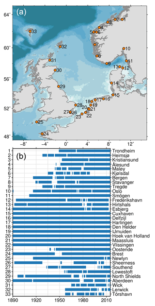
Figure 1 Locations of the tide-gauge stations and the availability of data at each station over the period 1890–2014. The numbers in panel (a) correspond to the numbers in panel (b).

We limit our tide-gauge data to the period 1890–2014 to avoid the inclusion of the sea-level jump that is apparent in many Dutch tide-gauge stations around 1885. From that year, monthly mean sea level is based on mean sea-level readings rather than mean tide level readings, which could result in a jump in the monthly data (Woodworth, 2017a). According to the PSMSL documentation, a correction has been applied to avoid this jump, but the jump is not apparent in some neighbouring stations and, as such, suspect. We only consider years for which at least 10 months of data is available. Starting from the monthly tide-gauge data, we compute seasonal sea-level anomalies as follows. First, we remove the annual-mean sea level from the monthly data. To ensure that each season consists of consecutive months, each year runs from December of the year before until November. Then, gaps of 2 months and shorter are linearly interpolated. The resulting monthly time series is then separated into seasonal deviations for four seasons: winter (December, January, February – DJF), spring (March, April, May – MAM), summer (June, July, August – JJA), and autumn (September, October, November – SON). The monthly sea-level data are averaged over each season, which results in four sea-level anomalies per year – one for each season. The resulting sea-level time series are thus seasonal deviations from annual mean sea level. Annual sea level can be affected by a large deviation in a particular season (e.g. a winter with very high sea level results in a higher annual mean), which in that case will result in an anomaly with an opposite sign during the other seasons. We have followed this approach instead of removing the linear trend or the low-frequency component from the tide-gauge data because in this region, the aforementioned baroclinic response to longshore wind forcing causes a large interannual variability signal, which would leak into the seasonal anomalies if only the linear trend or low-frequency variability instead of the annual mean is removed.

To obtain continuous records of wind stress and sea-level pressure anomalies, we use monthly-mean output from the NOAA 20th-century reanalysis project version V2C (Compo et al., 2011). To obtain seasonal deviations from the annual-mean values, we follow the same procedure as with the tide-gauge data: we remove the annual-mean and group the monthly anomalies into season-average anomalies. We compute wind stress from the 10 m wind speeds using the following relation

$$\begin{array}{}\text{(1)}& {\displaystyle }{\mathit{\tau }}_u& {\displaystyle }={\mathit{\rho }}_{\mathrm{air}}{C}_{\mathrm{D}}u\sqrt{u^{\mathrm{2}}+v^{\mathrm{2}}},\text{(2)}& {\displaystyle }{\mathit{\tau }}_v& {\displaystyle }={\mathit{\rho }}_{\mathrm{air}}{C}_{\mathrm{D}}v\sqrt{u^{\mathrm{2}}+v^{\mathrm{2}}},\end{array}$$

where ρ_air is the density of air, u and v the zonal and meridional 10 m wind velocity, and C_D the drag coefficient, which is parameterised following Pugh and Woodworth (2014):

$$\begin{array}{}\text{(3)}& C_{\mathrm{D}}=\mathrm{0.8}+\mathrm{0.065}\sqrt{u^{\mathrm{2}}+v^{\mathrm{2}}}.\end{array}$$

We parameterise the effects of seasonal local wind stress and sea-level pressure on sea level as a linear model:

$$\begin{array}{}\text{(4)}& {\mathit{\eta }}_{\text{obs}}={\mathit{\alpha }}_{\mathrm{0}}+{\mathit{\alpha }}_{\mathrm{1}}{p}^{\prime }\left(t\right)+{\mathit{\alpha }}_{\mathrm{2}}{\mathit{\tau }}_u\left(t\right)+{\mathit{\alpha }}_{\mathrm{3}}{\mathit{\tau }}_v\left(t\right)+\mathit{ϵ}\left(t\right).\end{array}$$

In this model, η_obs is the observed seasonal sea-level deviation, t is the time of the observation, p^′(t) is the local sea-level pressure anomaly, τ_u(t) the zonal wind stress, τ_v(t) the meridional wind stress, and ϵ(t) the residual. We obtained the pressure anomalies and wind stress values by taking the model value with the highest correlation coefficient within a 500 km radius around each tide-gauge station. We solve this system using ordinary least squares, which gives us the regression parameters [α₀ … α₃]. We test for the significance of each regressor using a t-test statistic and only include regressors for which the accompanying 95 % confidence interval does not cross zero. Since the individual regressors could be mutually correlated, we apply a stepwise regression scheme. We start with the regressor that has the highest (absolute) correlation with the seasonal sea-level deviations and subsequently add the extra regressors, ranked by their correlation. We only consider regressors for which the adjusted R² statistics increases after inclusion of that regressor. The adjusted R² statistic determines whether the extra regressor results in a significantly higher fraction of explained variance and is defined as

$$\begin{array}{}\text{(5)}& {\widehat{R}}^{\mathrm{2}}=\mathrm{1}-\left(\mathrm{1}-R^{\mathrm{2}}\right){\displaystyle \frac{n-\mathrm{1}}{n-p-\mathrm{1}}},\end{array}$$

with n the number of available season years, and p the number of included regressors. R² is the fraction of explained variance, which is defined as

$$\begin{array}{}\text{(6)}& R^{\mathrm{2}}=\mathrm{1}-{\displaystyle \frac{\mathrm{var}({\mathit{\eta }}_{\text{obs}}-{\mathit{\eta }}_{\text{exp}})}{\mathrm{var}({\mathit{\eta }}_{\text{obs})}}},\end{array}$$

with var() the variance operator and η_exp the sea-level deviations explained by the regression models.

Figure 2 Standard deviation of the seasonal sea-level anomalies for each season after applying a 10-year low-pass filter at all tide-gauge locations.

To obtain a link between coastal sea level and large-scale atmospheric patterns over the North Atlantic Ocean, we have computed the three leading principal components of the sea-level pressure field from the 20th-century reanalysis following the procedure described in Chafik et al. (2017). The monthly gridded sea-level pressure field between 80^∘ W–50^∘ E and 30–80^∘ N is selected, the linear trend, the annual cycle and the semi-annual cycle are removed, and from the resulting field, the three leading empirical orthogonal functions and associated principal components have been computed. We have chosen the method from Chafik et al. (2017) over selecting the original indices to obtain a coherent set of large-scale atmospheric variability from a single data source. Note that removing the semi-annual and annual cycle does remove the mean cycles themselves but not the low-frequency variability around the mean cycles, which is the quantity we are interested in.

From the monthly principal components, we compute seasonal anomalies by first removing the annual mean from the monthly data, and are subsequently average the monthly data into seasonal anomalies. As with the effects of local winds and pressure changes, we compute the effect of large-scale atmospheric variability on local sea level using a linear regression model

$$\begin{array}{}\text{(7)}& {\mathit{\eta }}_{\text{obs}}={\mathit{\beta }}_{\mathrm{0}}+{\mathit{\beta }}_{\mathrm{1}}{\mathrm{PC}}_{\mathrm{1}}\left(t\right)+{\mathit{\beta }}_{\mathrm{2}}{\mathrm{PC}}_{\mathrm{2}}\left(t\right)+{\mathit{\beta }}_{\mathrm{3}}{\mathrm{PC}}_{\mathrm{3}}\left(t\right)+\mathit{ϵ}\left(t\right),\end{array}$$

in which PC_n(t) is the nth principal component. The regression coefficients, [β₀…β₃] are estimated using ordinary least squares using the same stepwise regression approach as used for the local wind and pressure model.

To obtain information on low-frequency variability, we use a second-order Butterworth low-pass filter with a cutoff period of 10 years. Note that the regression models are applied to unfiltered data and that the filters have been applied as a post-processing step. To estimate trends in seasonal sea-level deviations, we use the Hector software (Bos et al., 2013), which computes the trend and the 1σ confidence intervals under the assumption that the residuals can be described by a first-order autoregressive (AR₁) process.

3 Results

The first objective of this paper is to quantify low-frequency seasonal variability for each season, which is shown in Fig. 2. This figure depicts the standard deviation of the low-pass-filtered seasonal sea-level time series, which is a measure of the typical amplitude of the multi-decadal variability in seasonal sea level.

The figure shows that the low-frequency seasonal variability in winter and autumn is generally larger than in summer and spring for most stations, with the winter-mean variability being the largest. The amplitude of low-frequency winter and autumn variability shows a clear regional pattern: high variability can be found in the German Bight, the Skagerrak between Norway and Denmark, as well as along the Norwegian coast towards the north, while for the southern North Sea, Brest, Newlyn, and the British coast, this variability is smaller. Although the low-frequency variability in spring and summer is substantially smaller than in winter, the spatial patterns for each season show some similarities: also in spring and summer, the variability is highest for the stations surrounding the German Bight. The southeastern North Sea is a hotspot for low-frequency variability in the region, but the differences between seasonal and annual sea-level variability found by Dangendorf et al. (2013) for the Cuxhaven station are not a purely local phenomenon. This low-frequency variability can be interpreted as trends when short records are used. To quantify typical trends that could emerge from low-frequency variability in season-mean sea level, we have computed 40-year running mean trends in seasonal sea level deviations for four stations. The resulting trends are depicted in Fig. 3.

Figure 3 Running-mean trends in seasonal sea level deviations for four stations, using a 40-year window. Trends are only shown for time windows with at least 30 years of data. The shading denotes the 1σ confidence interval. Note that these trends have been computed from the time series without the low-pass filter applied. The numbers in the legend correspond to the station numbers in Fig. 1

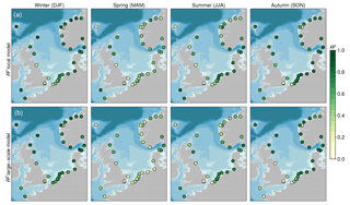
Figure 4 Fraction of 10-year low-pass-filtered seasonal variance (R²) explained by the local (a) and large-scale model (b) for each station.

For all seasons, the trends in seasonal sea level can reach values in the same range of the secular trend in geocentric mean sea level, which is typically in the order of 1–2 mm year⁻¹ for this region (Wahl et al., 2013), with the largest 40-year trends occurring during autumn and winter. The confidence intervals for these 40-year trends are in the order of 1 mm year⁻¹. For Oslo and Cuxhaven, the seasonal trends sometimes reach values in the order of 4 mm year⁻¹, which is about twice the rate of the secular trend. This variability in seasonal deviations could also be interpreted as an acceleration: for example, the trend in winter sea-level deviations in Oslo and Cuxhaven is generally higher in the last few decades than in the first few decades, which could translate into a long-term positive acceleration in the seasonal sea-level deviation time series. Again, note that these trends are trends in seasonal deviations from annual-mean sea level, and they do not represent secular trends in sea level.

To determine whether local wind and pressure changes are responsible for this variability, we compute the fraction of explained variance (R²) of the local regression model (Eq. 4) after applying a 10-year low-pass filter to both the seasonal sea-level deviations and the solution to the regression model. The results are depicted in the top row of Fig. 4.

In autumn and winter, when the low-frequency variability is highest, the local regression model explains a large fraction of the variability for most stations. Especially in the winter (DJF) season, the model explains the majority of the observed variability (R²>0.5) for most stations. In spring and summer, generally a smaller part of the variability can be explained, which suggests that the long-term seasonal variability, which is already much smaller than the winter and autumn variability, is less predominantly driven by wind and pressure changes. However, for some stations, such as Brest and Newlyn, the local regression model explains the majority of the variability for all seasons.

Local wind and pressure variability are affected by large-scale atmospheric circulation patterns, such as the NAO and EAP. The next step is to investigate whether the multi-decadal variability in seasonal sea level deviations can be explained by the low-frequency variability in these large-scale patterns. To this end, we use the three leading principal components of surface pressure variability, as described in Sect. 2. These principal components and their associated empirical orthogonal functions represent the major patterns of atmospheric variability and are displayed in Fig. 5. As such, they share characteristics with well-known atmospheric teleconnection patterns. The distinct north–south pattern of the first principal component resembles the North Atlantic Oscillation (Hurrell et al., 2003), while the second and third principal components (PCs) are akin to the East Atlantic Pattern and the Scandinavia Pattern respectively (Cassou et al., 2004). It must be noted that the principal components computed here are not fully interchangeable with the commonly used original indices, which are generally computed using different methods.

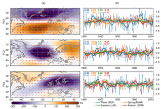
Figure 5 The first three empirical orthogonal functions (EOFs) and accompanying principal components (PCs) of sea-level pressure above the North Atlantic Ocean. Panel (a) shows the spatial patterns of each EOF. The red arrows depict the associated geostrophic wind vectors. Panel (b) shows the season-mean PCs (thin line) and the season-mean PCs after applying a 10-year low-pass filter. The variance of the monthly-mean principal components is scaled to 1, and the numbers in the top-left corner denote the low-pass-filtered variance (bold) and the unfiltered variance (regular) for each season. Multiplication of the EOF with the accompanying PC gives the resulting sea-level pressure anomaly in pascal.

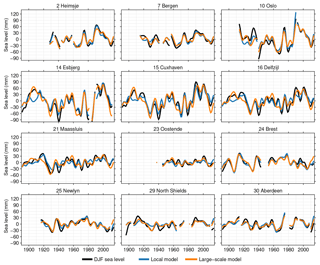
Figure 6 Time series of winter (DJF) sea level, the reconstructed sea level from the regression model, and the residual at selected tide-gauge stations. A 10-year low-pass filter has been applied to all time series.

The first EOF is associated with westerly winds over the whole North Sea Basin, while the second EOF shows a more meridionally oriented wind effect, albeit with a curvature over the North Sea. EOF3 has its centre of action over southern Scandinavia, and hence, the wind strength associated with this EOF shows a large north–south gradient over the North Sea, with stronger winds in the south. All three patterns show both season-to-season variability (thin lines in Fig. 5) as well as variability on multi-decadal scales (thick lines). For all three principal components, the variability in winter is the largest, both for the seasonal and for the low-pass-filtered time series. The difference is most pronounced for the first principal component, which is a well-known feature of the NAO (Hurrell et al., 2003), but it is visible in all three PCs for the seasonal and for the low-pass-filtered time series.

The three PCs are used in the large-scale regression model (Eq. 7), and the results are depicted in the bottom row of Fig. 4. Like the local regression model, the large-scale regression model also explains a large fraction of the multi-decadal variability in winter and autumn sea level, while for spring and summer, the explained fraction is generally smaller. Interestingly, for some stations in winter, especially for the stations in Belgium and in the southern part of the Netherlands, the large-scale model even explains more variability than the local model. This difference may have its cause in the complex wind and pressure patterns generated by the large-scale atmospheric patterns, which may not be well-captured by the single-point wind and pressure time series used in Eq. (4). For some other stations, such as Brest and Newlyn, the local model explains more variability than the large-scale model, suggesting that not all variability is driven by large-scale patterns, but local effects also play a role. The fact that both models explain a large fraction of the variability in autumn and winter shows that the variability is predominantly driven by wind and pressure changes that are linked to large-scale atmospheric patterns.

Not only the amplitude of the variability (Fig. 4) but also the temporal pattern differs between stations in this region, which can be seen in Fig. 6. This figure shows time series of long-term winter-mean sea-level variability together with the results from both regression models at 12 representative stations.

This figure again shows the major features of Figs. 2 and 4: high variability in the German Bight, low variability along the British coast and the southern North Sea, and the ability of both regression models to explain a large part of this variability. The pattern of variability shows differences over the region: the stations in the German Bight (Delfzijl, Cuxhaven, Esbjerg) and Oslo show a coherent variability pattern, which differs from the patterns found in other locations. For example, during the period 1985–2005, most stations along the eastern North Sea coast show an above-average sea level, which is much less pronounced along the British coast, and even corresponds to a drop in seasonal sea level for the stations Brest and Newlyn. For all these stations, both regression models explain these features, which shows that the differences between these stations must be caused by a difference in wind and pressure forcing, and consequently, the large-scale atmospheric patterns affect different stations in a different way, and the variability at different stations may be attributable to a different combination of influence from the large-scale patterns.

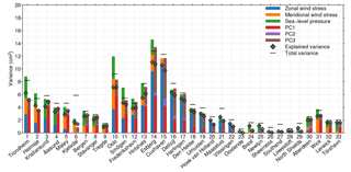
To understand these differences between the forcing mechanisms between the different stations, Fig. 7 shows the fraction of explained variance for each individual regressor and the full regression model of low-pass-filtered DJF sea level both in the local and large-scale regression models.

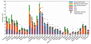
Figure 7 Total and explained variance of DJF sea level at each tide-gauge station. The left bar shows the variance explained by each term in the local model and the right bar the variance explained by the large-scale model. The explained variance is computed using the regression coefficients from the model with all accepted terms and not by only regressing each individual term. Negative fractions of explained variance are not shown. The total and explained variances were computed after applying a 10-year low-pass filter. The numbers on the lower axis correspond to the station numbers in Fig. 1.

Figure 8 Same as Fig. 7, but for the autumn (SON) season.

This figure shows that the origins of the forcing differ substantially throughout the region: while the stations from the German Bight towards the southern North Sea are dominated by zonal wind stress, the more northern stations are forced by a combination of zonal and meridional wind and sea-level pressure. At the other side of the English Channel, Brest and Newlyn are dominated by sea-level pressure effects. This is also the case for Tórshavn, which can be explained by the fact that Tórshavn is an off-shelf island, for which wind stress will not cause large storm surges due to the large ocean depth and the absence of a large ocean boundary. Along the northern Norwegian coast, which also shows a large variability signal, both zonal and meridional wind as well as surface pressure variability explain a large fraction of the variability.

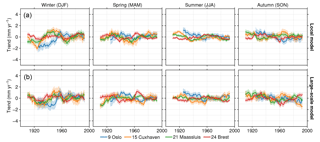
Figure 9 Running-mean 40-year trends in seasonal sea level deviations for four stations after removal of the local (a) and large-scale (b) models. The top panels show trends in the original time series, and the bottom row shows the trends Trends are only shown for time windows with at least 30 years of data. Note that these trends have been computed from the time series without the low-pass filter applied.

Despite the large regional variations in the local forcing agents, the first principal component PC1, which is closely tied to the North Atlantic Oscillation, explains the largest fraction of the variability for most stations. For the stations in the southern North Sea, which are less affected by the westerlies associated with this PC (see Fig. 5), the third PC explains a large part of the variability. The first PC is associated with both zonal, meridional, and pressure changes along the Norwegian coast, which explains the aforementioned impact of wind and pressure on the stations in that region. The third PC is associated with a strong zonal geostrophic wind component over the southern North Sea. The second PC explains a small part of the variance, even though the signal does contain a considerable decadal winter-mean signal. The only exceptions are Brest and Newlyn, where PC2 affects the zonal wind.

For the autumn season, different factors affect the low-frequency variability, as shown in Fig. 8.

In autumn, the variability, which is generally much smaller than in winter is generally driven by the same drivers as the winter variability, but the local wind and pressure variability is driven by a different combination of large-scale patterns for some stations, especially along the German Bight, where the seasonal variability is now mostly driven by the third PC instead of the first PC.

The trends in seasonal sea-level deviations, depicted in Fig. 3, are also to a large extent caused by the atmospheric forcing. Figure 9 shows the same trends in seasonal deviation but after removing sea-level deviations explained by the local and large-scale model.

For all seasons, the local and large-scale regression models explain a large fraction of the running-mean trends. For winter and autumn, after applying the regression models, the residual seasonal trends have the same order of magnitude as typical secular mean sea level trends, and the trend differences between the beginning and end of the considered periods have been substantially reduced. However, not all low frequency has been explained by the models, and the residual time series still contain trends and accelerations.

4 Conclusions

In this paper, we have analysed the low-frequency variability in the seasonal deviations from annual mean sea level in the North Sea region. Low-frequency variability in winter-mean and autumn-mean sea level shows a spatially varying pattern, with the highest values encountered along the German Bight. This variability is largely forced by wind and pressure. The wind generally plays a large role for locations that show large low-frequency variability, and the variability is indeed weaker where wind plays a minor role, e.g. the British North Sea coast. The low-frequency changes in local wind and pressure are linked to large-scale atmospheric patterns, which resemble the NAO, EAP, and Scandinavia Pattern. Hence, the low-frequency variability in large-scale atmospheric patterns translates into low-frequency winter-mean and autumn-mean sea-level variability. In spring and summer, the low-frequency variability is smaller and can generally be explained only to a small extent by local and large-scale atmospheric forcing.

This seasonal sea-level variability is mostly caused by wind and pressure changes. Therefore, extreme sea levels associated with storm surge events are not superimposed onto this variability. In other words: a storm that occurs during a “low phase” will not generate a lower surge level than when the same storm occurs during a “high phase”. Because the sea-level response to local wind and pressure changes in the North Sea is mostly barotropic in nature (Chen et al., 2014; Dangendorf et al., 2014a), the typical sea-level adjustment timescale to wind and pressure changes will not be longer than a few days (Dimon et al., 1997). However, the sea-level response to atmospheric forcing is mostly, but not necessarily fully barotropic in the North Sea (Calafat et al., 2012; Tsimplis et al., 2006), and local and large-scale atmospheric changes do not explain all variability. For example, processes like ocean circulation changes and low-frequency variability in freshwater fluxes from rivers and locks (Gerkema and Duran-Matute, 2017) could drive low-frequency sea-level deviations. As such, seasonal sea-level changes could still play a role in variability in storm-surge heights.

Multi-decadal seasonal sea-level variability in the North Sea is of the same order of magnitude as the long-term trend in mean sea level, and as a result, multi-decadal trends in annual mean sea level are in general not representative of the trends of the winter record in isolation. For processes that rely on long-term sea level variability, for example coastal sand suppletion, this difference needs to be taken into account. Furthermore, seasonal wind and pressure effects will eventually influence annual-mean sea-level variations. Since a large part of the variability can be explained by a simple regression model, this correction should not pose a challenge.